

Simple and robust algorithms to estimate liveweight in African smallholder cattle
J. P. Goopy A C D , D. E. Pelster A , A. Onyango A B , K. Marshall A and M. Lukuyu CA Mazingira Centre, International Livestock Research Institute, PO Box 0110, Nairobi, Kenya.
B University of Hohenheim, Schloß Hohenheim 1, PO Box 30709, 00100, Stuttgart 70599, Germany.
C University of New England, Trevanna Road, Armidale, NSW 2351, Australia.
D Corresponding author. Email: j.goopy@cgiar.org
Animal Production Science 58(9) 1758-1765 https://doi.org/10.1071/AN16577
Submitted: 23 August 2016 Accepted: 16 March 2017 Published: 17 May 2017
Journal compilation © CSIRO 2018 Open Access CC BY-NC-ND
Abstract
Measurement of liveweight of stock is one of the most important production tools available to farmers – playing a role in nutrition, fertility management, health and marketing. Yet most farmers in sub-Saharan Africa do not have access to scales on which to weigh cattle. Heart girth measurements (and accompanying algorithms) have been used as a convenient and cost-effective alternative to scales, however despite a plethora of studies in the extant literature, the accuracy and sensitivity of such measures are not well described. Using three datasets from phenotypically and geographically diverse cattle populations, we developed and validated new algorithms with similar R2 to extant studies but lower errors of prediction over a full range of observed weights, than simple linear regression, that was valid for measurements in an unassociated animal population in sub-Saharan Africa. Our results further show that heart girth measurements are not sufficiently sensitive to accurately assess seasonal liveweight fluctuations in cattle and thus should not be relied on in situations where high precision is a critical consideration.
Additional keywords: allometric, heart girth, prediction error, sub-Saharan Africa.
Introduction
Measurement of liveweight (LW) and LW change is ubiquitous to most aspects of ruminant livestock husbandry and management. In advanced agricultural systems, assessment of LW is indispensable in measuring growth, estimating intake and nutritional requirements of stock and determining their readiness for market or for joining (Sawyer et al. 1991). Measurement of LW is also requisite in the determination of more complex factors such as food conversion efficiency and residual feed intake, which are gaining importance in advanced livestock production systems (e.g. Veerkamp 1998).
On a simpler, but equally important level, knowledge of LW is essential for safe and efficacious administration of veterinary medications and for farmers to receive an equitable price in the sale of animals. Calibrated weighing scales are considered the gold standard for determining LW, but these are rarely available to smallholder farmers in sub-Saharan Africa (SSA). Often, the only recourse that farmers have is to estimate the LW of their animals visually, but Machila et al. (2008) has demonstrated that farmers are poor judges of their animals’ LW and further, that some commercially produced ‘weigh bands’ (e.g. CEVA Santé Animale) consistently overestimate LW of smallholder cattle, suggesting that the algorithm on which the graduations of the weigh band are based are not valid to use in such populations. Irrespective of this, heart girth circumference measurements (HG) have been consistently demonstrated across many studies to have a strong, although variable, correlation with LW (Table 1). This variability may be due to phenotypic differences between populations, but is rarely explored (e.g. Buvanendran et al. (1980)) and there has been apparently little interest in developing a more universally applicable algorithm for Zebu × cattle in SSA. Several studies have considered other allometric measurements (e.g. wither height, body length, body condition score), but such additional measurements have not greatly improved the relationship of LW to HG (Buvanendran et al. 1980; Bozkurt 2006; Bagui and Valdez 2009). Thus HG has been repeatedly demonstrated to be the most useful and robust proxy for the use of scales in the LW estimation of cattle.

|
Studies that explored quadratic and exponential relationships between HG and LW (Buvanendran et al. 1980; Nesamvuni et al. 2000; Francis et al. 2004), have not improved coefficients of regression by more than a few percentage points, while having added unneeded complexity to the model. Perhaps because the simplest relationship appears (based on R2) to be as strong as the more complex equations, the relationship between HG and LW has generally been described by simple linear regression (Table 1).
Using the coefficient of determination of a regression as the criterion for goodness-of-fit does not provide information about variance or bias in the model, and hence the degree to which the values predicted by the model will vary from true values. The magnitude of the prediction error (PE) will critically affect the utility of using HG measurements to estimate LW. Although PE of 20% may be acceptable for setting dosage rates for veterinary chemicals (Leach and Roberts 1981), errors of 10% or greater are problematic when using HG measurements to assess production-related traits in individual animals that require accurate LW determination. Lesosky et al. (2012), taking a different approach – transforming the response variable while using a simple linear regression, reported PE of less than 20% with a co-efficient of determination of 0.98. This study was based on a group of phenotypically similar indigenous Zebu cattle of limited weight range (mostly <100 kg) and it is unclear whether such a strong relationship would be observed in a more phenotypically diverse population.
Therefore, our study had four objectives:
-
To determine the strongest relationship possible between HG and LW, by considering both PE and regression coefficients, rather than regression coefficients alone;
-
To determine the extent to which disaggregation of data into more phenotypically homogenous populations is likely to strengthen the relationship between HG and LW;
-
To assess whether such an algorithm may be used successfully to establish LW in novel populations; and
-
To determine the applications for which HG measurements may validly be used as an alternative to weighing scales for LW determination.
Materials and methods
Animal population for algorithm development
Two datasets, one each from West and East Africa were used to develop and train the HG algorithm. The East African dataset comprised smallholder (Zebu × Bos taurus) female crossbred dairy cattle in Siongiroi (0°55ʹS, 35°13ʹE; ~1800 m above sea level) and Meteitei (00°30ʹN, 35°17ʹE; ~2000 m above sea level) districts of Rift Valley Province, and Kabras district in Western Province (00°15ʹ10°N, 34°20ʹ35°E: ~1500 m above sea level; (n = 439, LW: range: 36–618 kg, × = 264.9 kg, s.e.m. = 3.74 kg) (Lukuyu et al. 2016). Data from cattle from West Africa were collected between November 2013 and June 2015 on 84 farms in the Thiès and Diourbel regions of Senegal, (n = 621, LW: range: 31–604 kg; × = 262.7 kg, s.e.m. = 4.06 kg) with the different breed/cross-breeds of cattle in the study sample were assigned to four main breed-groups (i.e.: (i) indigenous Zebu, (ii) Zebu × Guzerat, (iii) Zebu × B. taurus, (iv) predominantly B. taurus) either on the basis of farmer recall or, where available, genotype information (Tebug et al. 2016). All animals from each study had LW assessed gravimetrically using digital electronic weigh scales and HG measured simultaneously.
Analytical approach
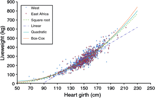
(i) The two datasets were examined both separately and in combination. These datasets were analysed and plotted using HG as the predictor variable and the measured LW as the response variable (Fig. 1).
|
We compared the West and East African populations using analysis of covariance (ANCOVA: using the AOV function in the software page R version 3.0.3, (R Development Core Team, 2010) on the entire population using the region (East vs West Africa) as a fixed factor and HG as a co-variant. To facilitate comparison with other studies (Table 1) we first used a simple linear regression model (SLR) to predict LW using HG (1).

We then considered five other relationships including log-transformation and quadratic equations as methods to minimise PE, but decided on the three models that appeared to produce the strongest relationships between LW and HG. The first was a square-root transformation of LW using a simple linear regression model (SQRT-LR) (2).

The second also transformed the response variable using a likelihood maximised Box–Cox transformation, h(y, λ) = (yλ – 1)/λ, λ = 0, to estimate the power coefficient to estimate the power coefficient (Box and Cox 1964). The power coefficient was determined using the Box–Cox function in R, using boundaries of –1 and 1 and a step of 0.001. The transformed LW was then used in a linear regression (BOXCOX-LR) (3).

The final model examined was a quadratic equation (QUAD) (4).

Model goodness-of-fit was analysed using the adjusted R2, (after back transforming the transformed response variables) and through examination of residual plots, normal probability plots and leverage plots. The residual plots were used to identify points with large associated residuals (possible outliers), whereas the normal probability plot was used to check linearity and normality assumptions. The leverage plots were used to detect data points with unusually high influence (Cook 1977). Outliers noted on the diagnostic plots were investigated and either corrected when possible (i.e. simple transcription error) or removed and the resulting dataset was re-analysed. In total, only 4 of the 1064 data points were removed. In addition to R2 we estimated PE ((ABS (measured LW – predicted LW))/measured LW) as well as the root mean squared error (RMSE). The two datasets plus the aggregated set were analysed using cross validation techniques as follows: datasets were split into two; 70% of the measurements were used to train the model (training set), whereas the other 30% were used to validate the model (validation set). The 75th, 90th and 95th percentiles for PE (i.e. what is the percent error required to capture 75%, 90% or 95% of the measurements) were calculated. The cross validation for each model (Eqns 1–4) and each dataset were repeated 1000 times using different splits for the cross validation each time, and descriptive statistics (X, s.d., coefficent of variation (c.v.)) were calculated for the PE 75th, 90th and 95th percentiles, model coefficients and adjusted R2. The PE were then used in conjunction with the previous criteria given above to determine the ability of each model type to accurately predict LW from the HG measurement.
Model validation
To address experimental aim (iii) we employed a further dataset derived from a mixed (Zebu and Zebu × B. taurus) smallholder cattle population in the Nyando Basin, Western Kenya (0°13ʹ30ʹʹS–0°24ʹ0ʹʹS, 34°54ʹ0ʹE–35°4ʹ30ʹʹE; 1200–1750 m above sea level n = 892, LW: range: 11.6–361.6 kg, × = 165.0 kg, s.e.m.: 1.45 kg; A. Onyango, pers. comm.). In total 1890 measurements were used (some animals were measured 2–4 times) as a secondary validation set. Using the parameters estimated from each of the models tested here and three models from other published studies, two using SLR (Msangi et al. (1999), Kashoma et al. (2011)) and the Lesosky et al. (2012) Box–Cox transformation linear regression, we calculated the expected LW from the HG measurements. We then calculated the 75th, 90th and 95th percentiles of the PE (i.e. the percent error that contains 75%, 90% or 95% of the correct LW). Again, diagnostic plots were used to identify outliers (data points with unusually high residual values, or high leverage), which were either corrected when possible or removed. There was a total of 11 data points removed from this dataset, resulting in 1879 data points being used for model validation.
As well as being useful for detecting outliers, the diagnostic plots also provide a useful visualisation of how well the model ‘fits’ the data. Normal probability (Q-Q) and standardised residual (residual/s.d. of residuals) plots show whether there is a systematic bias in the model, whereas the leverage plots provide an indication of the resilience of a model against outliers. Therefore, we also used these plots as a qualitative measure of each model.
Results
The datasets considered for the present study, differed from the data used in the studies of both Lukuyu et al. (2016) (LW = 102–433 kg) and Tebug et al. (2016). (LW = 110–618 kg) in that both of these used attenuated datasets in their analysis (compared with the original, or full dataset), eliminating particularly animals of low LW, which had implications in terms of the linearity of the relationship between LW and HG.
Diagnostics
Examination of the diagnostic plots for the linear regression model (e.g. residual and standardised residual plots) revealed that at the tails of the dataset (i.e. very small or very large animals) there was a strong bias towards positive residuals indicating a systematic underestimation of the animals’ LW (Fig. 2a).

|
This systematic bias was not present in the SQRT-LR (Fig. 2b), BOXCOX-LR (Fig. 2c) or the QUAD models (Fig. 2d) suggesting that these equations more accurately reflect true measurements, particularly at the extremes of low and high weights.
Leverage plots indicate the degree to which a single data point can alter the model and are therefore useful for examining the relative robustness of different models to outliers. As shown in Fig. 3, the QUAD model has points with leverage scores four times greater than those in the other three models.

|
All four of the models had adjusted R2 greater than 0.8, however the values for the SQRT-LR, BOXCOX-LR and QUAD models were all ~0.05 (5%) greater than the SLR (Table 2). The RMSE for the two transformed and the QUAD model were all similar and ~8% less than the SLR model (Table 2). PE for all models were similar at the 75th percentile, but importantly, both the two transformed (SQRT-LR, BOXCOX-LR) and the QUAD model had PE of up to 9% less at the 95th percentile compared with the SLR model, in both aggregated and disaggregated datasets.

|
The SQRT-LR, BOXCOX-LR and QUAD models were also significant when the dataset was disaggregated into the East and West African populations, with the adjusted R2 values ranging between 0.797 and 0.881 and the RMSE ranging between 34.2 and 36.9 (Table 2). Similar to the models run with the full dataset, SQRT-LR, BOXCOX-LR and QUAD models had higher adjusted R2, lower RMSE and lower PE (Table 2) than the SLR model indicating that they again tended to fit the data more accurately, which was likely due to the poor fit of the SLR at the extremes of the LW range.
However, disaggregating the combined dataset did not improve the model substantially, in fact, the adjusted R2 for the East African dataset decreased compared with the full dataset (Table 2). This was in agreement the results of the ANCOVA, which showed that population was not a significant factor for the SLR (P = 0.675), BOXCOX-LR (P = 0.706) or SQRT-LR (P = 0.886) models. This suggests that the two populations, although geographically and phenotypically divergent were similar enough to be considered a single population where LW can be effectively predicted by using the same HG algorithm(s) (refer also Fig. 1).
Model validation
Applying the parameters estimated from each of the models tested here and three models from other published studies using the aggregated dataset to the novel (validation) dataset produced mixed results. Applying the SLR model from our own study, and simple linear models from two other published studies (Msangi et al. 1999; Kashoma et al. 2011) produced similar, moderate-adjusted R2 (0.47–0.59), and PE of over 70% at the highest percentiles of PE (Table 3). In comparison, the more complex models (SQRT-LR, BOXCOX-LR, QUAD) and the model of Lesosky et al. (2012), displayed high adjusted R2 (0.91–0.92) and low PE across all percentiles (Table 3).

|
Discussion
Algorithms using HG to predict LW in cattle have been repeatedly demonstrated to be robust, with R2 of 0.75–0.85 and simple measures of fit, such as R2 or RMSE, are often assumed to be a reflection of the models’ predictive capacity and precision. However, the use of diagnostic plots to evaluate goodness-of-fit in models has revealed systematic biases in the use of SLR, not evident from the use of coefficients of determination as measures of fit alone. This is most apparent at the extremes of weight range (i.e. calves and mature animals), which may be why other studies examined the weight range. The calculated PE of 37% of LW under optimised conditions for the SLR suggests that the relationship between HG and LW is not a simple, linear one and that SLR equations are not particularly useful in describing the relationship between HG and LW or in the accurate estimation of LW when considering the full range of LW observed in smallholder cattle populations.
In contrast, transforming the response variable or using a quadratic equation to describe the relationship between HG and LW, both eliminates systematic bias (as indicated in diagnostic plots, see also Figs 2, 3), particularly noticeable at either extreme, and markedly improves the accuracy of LW estimates.
Intuitively, population characteristics that influence animal morphology, such as breed (type), sex, degree of maturity or body condition score, might be assumed to alter the relationship between HG and LW, and many studies have disaggregated and analysed their data by one or more of these characteristics (see Table 1 for examples). That such differences exist is clear from the different algorithms derived within single populations; however, this presents practical problems if the object is to use the algorithms so derived to estimate LW in other animals, more so if the population(s) to be assessed are different from the population the equations were derived from.
In this study, we deliberately set out to determine if a widely applicable algorithm using HG as the single dependent variable could be developed to accurately estimate LW in a novel population. Our starting point was to use two geographically separate populations that differed in breed/type and LW makeup, and we clearly showed that, despite these differences they could be considered as one population for the purposes of determining the relationship between HG and LW. Despite producing different algorithms when the populations were separated, this did not improve the strength of the relationship, or reduce the (prediction) error in any meaningful way. However, we also noted that the SLR equations developed from the datasets we used, showed lower R2 than the values published by Lukuyu et al. (2016) and Tebug et al. (2016). We infer from this and the graphical structure of the HG/LW distribution (Fig. 1), that this is a result of our equations being derived from the full range of LW and demonstrates the non-linearity of HG/LW over the full LW range.
Applying the algorithms we developed to our validation dataset highlighted two key points. First, although the validation dataset was probably reasonably similar to the (aggregated) development population, being a mixture of indigenous and crossbred cattle (but with a different LW range), applying both our SLR equation and those from two other published studies, produced such large (72–87%) PE as to make them inapplicable for practical purposes. In contrast, applying the more complex algorithms from our study (SQRT-LR, BOXCOX-LR, QUAD) and the Box–Cox transformation of Lesosky et al. (2012), all produced PE of less than 25% at the highest percentile, with the Box–Cox transformations and QUAD algorithm showing the lowest PE (18–19%), indicating that such equations may be able to be validly applied in other, novel populations. Of these, the quadratic model (QUAD) is possibly less useful given the likely influential effect of small subsets of a population on the equations developed and the increased complexity of the model does not noticeably improve either the fit (R2) or the prediction accuracy.
The reasons that the PE of the transformed equations are even lower in the validation dataset (than the development set) are difficult to define. One reason may be that the LW of the validation set occurred over a smaller range compared with the development dataset, and thus showed less variability than the development dataset. A second reason may be that measurements taken in the validation population were all made by one experienced operator and so had lower operator (random) error.
Irrespective of this, it is clear that using either a quadratic model (QUAD) or a square-root (SQRT-LR) or Box–Cox (BOXCOX-LR) transformation (of the response variable) in a linear regression, makes the prediction of LW from HG more reliable over the full range of observed LW, considerably reducing bias and PE. Further, considering the results observed in applying those algorithms to our validation dataset it appears that the algorithms developed from this dataset may be widely applicable, at least to the types of cattle typically held by sedentary smallholder farmers, although further exploration is needed to confirm this.
There are limitations to the utility of HG in estimating LW however. PE of ~25% (at the 95th percentile) indicate that the HG/LW relationship using non-SLR equations is sufficiently accurate to be used in veterinary applications and are much better than farmer visual-assessment estimates (Machila et al. 2008). It is important to recognise however that our improved HG-derived estimates are still not sufficiently sensitive to reliably capture relatively small changes in LW, such as those commonly observed seasonally in smallholder cattle, (observed to be in the range of 11–17% of LW; A. Onyango, pers. comm.) and conventional scales will continue to be required to capture data of this sort.
Conclusion
The HG measurements, although demonstrably inferior to gravimetric methods for assessing LW, have clear advantages of accessibility and ease of use. We have optimised HG algorithms, significantly reducing PE associated with HG-derived estimates of LW. The improved algorithms may be used with higher confidence for animal health applications and to assist farmers in decision-making – in feed formulation, marketing, joining or other husbandry-related issues. The algorithms using a transformed response variable, (Box–Cox, or square-root transformation) or quadratic equations developed in this study, may also be applied directly to other populations of smallholder cattle in SSA, without the need to undertake extensive testing and further development of new algorithms for each new population of interest.
Improving LW estimation (through improving the accuracy of HG-derived measurements) has the potential to improve the livelihoods of smallholders in Africa through allowing farmers to make better-informed management decisions regarding their animals. It is also clear that estimates of LW from HG measurements are limited in their accuracy, despite improvements and are not of sufficient precision to capture the seasonal variations in LW that may be of interest from a research perspective or to be an equivalent alternative to well-calibrated weighing scales, where such an option exists.
Acknowledgements
Funding for this study was provided by the German Federal Ministry for Economic Cooperation and Development (BMZ) and the German Technical Cooperation (GIZ) as part of their program: ‘Green innovation centres for the agriculture and food sector’ and the project ‘In situ assessment of GHG emissions from two livestock systems in East Africa – determining current status and quantifying mitigation options’. A. Onyango was supported by a scholarship granted by the German Academic Exchange Service (DAAD). M. Lukuyu’s study was funded by the Dairy Genetics East Africa (DGEA) project, a collaboration between the University of New England and the International Livestock Research Institute funded by the Bill and Melinda Gates Foundation. We further acknowledge the CGIAR Fund Council, Australia (ACIAR), Irish Aid, European Union, International Fund for Agriculutrual Development (IFAD), Netherlands, New Zealand, UK, USAID and Thailand for funding to the CGIAR Research Program on Climate Change, Agriculture and Food Security (CCAFS).
References
Bagui NoJG, Valdez CA (2009) Live weight estimation of locally raised adult purebred Brahman cattle using external body measurements. Philippine Journal of Veterinary Medicine 44,Box GEP, Cox DR (1964) An analysis of transformations. Journal of the Royal Statistical Society. Series B. Methodological 26, 211–252.
Bozkurt Y (2006) Prediction of body weight from body size measurements in brown Swiss feedlot cattle fed under small-scale farming conditions. Journal of Applied Animal Research 29, 29–32.
| Prediction of body weight from body size measurements in brown Swiss feedlot cattle fed under small-scale farming conditions.Crossref | GoogleScholarGoogle Scholar |
Branton C, Salisbury GW (1946) The estimation of the weight of bulls from heart girth measurements. Journal of Dairy Science 29, 141–143.
| The estimation of the weight of bulls from heart girth measurements.Crossref | GoogleScholarGoogle Scholar |
Buvanendran V, Umoh JE, Abubakar BY (1980) An evaluation of body size as related to weight of three West African breeds of cattle in Nigeria. The Journal of Agricultural Science 95, 219–224.
| An evaluation of body size as related to weight of three West African breeds of cattle in Nigeria.Crossref | GoogleScholarGoogle Scholar |
Cook RD (1977) Detection of influential observation in linear regression. Technometrics 19, 15–18.
Francis J, Sibanda S, Kristensen T (2004) Estimating body weight of cattle using linear body measurements. Zimbabwe Veterinary Journal 33, 15–21.
| Estimating body weight of cattle using linear body measurements.Crossref | GoogleScholarGoogle Scholar |
Goe MR, Alldredge JR, Light D (2001) Use of heart girth to predict body weight of working oxen in the Ethiopian highlands. Livestock Production Science 69, 187–195.
| Use of heart girth to predict body weight of working oxen in the Ethiopian highlands.Crossref | GoogleScholarGoogle Scholar |
Kashoma I, Luziga C, Werema C, Shirima G, Ndossi D (2011) Predicting body weight of Tanzania shorthorn zebu cattle using heart girth measurements. Livestock Research for Rural Development 23, 94
Leach TM, Roberts CJ (1981) Present status of chemotherapy and chemoprophylaxis of animal trypanosomiasis in the eastern hemisphere. Pharmacology & Therapeutics 13, 91–147.
| Present status of chemotherapy and chemoprophylaxis of animal trypanosomiasis in the eastern hemisphere.Crossref | GoogleScholarGoogle Scholar | 1:CAS:528:DyaL3MXkvFSltL4%3D&md5=b3d365e876c8c1d40fec472edf589658CAS |
Lesosky M, Dumas S, Conradie I, Handel IG, Jennings A, Thumbi S, Toye P, de Clare Bronsvoort BM (2012) A live weight–heart girth relationship for accurate dosing of east African shorthorn zebu cattle. Tropical Animal Health and Production 45, 311–316.
| A live weight–heart girth relationship for accurate dosing of east African shorthorn zebu cattle.Crossref | GoogleScholarGoogle Scholar |
Lukuyu MN, Gibson JP, Savage DB, Duncan AJ, Mujibi FDN, Okeyo AM (2016) Use of body linear measurements to estimate liveweight of crossbred dairy cattle in smallholder farms in Kenya. SpringerPlus 5, 63
| Use of body linear measurements to estimate liveweight of crossbred dairy cattle in smallholder farms in Kenya.Crossref | GoogleScholarGoogle Scholar | 1:STN:280:DC%2BC28nnt1OntA%3D%3D&md5=a800b3a1e19f012d4d3040019b724afaCAS |
Machila N, Fèvre EM, Maudlin I, Eisler MC (2008) Farmer estimation of live bodyweight of cattle: implications for veterinary drug dosing in East Africa. Preventive Veterinary Medicine 87, 394–403.
| Farmer estimation of live bodyweight of cattle: implications for veterinary drug dosing in East Africa.Crossref | GoogleScholarGoogle Scholar |
Msangi B, Bryant M, Kavana P, Msanga Y, Kizima J (1999) ‘Body measurements as a management tool for crossbred dairy cattle at a Smallholder farm condition, Proceedings of the 26th Scientific Conference of the Tanzania Society of Animal Production.’
Nesamvuni A, Mulaudzi J, Ramanyimi N, Taylor G (2000) Estimation of body weight in Nguni-type cattle under communal management conditions. South African Journal of Animal Science 30, 97–98.
Sawyer G, Barker D, Morris R (1991) Performance of young breeding cattle in commercial herds in the south-west of Western Australia. 2. Liveweight, body condition, timing of conception and fertility in first-calf heifers. Australian Journal of Experimental Agriculture 31, 431–441.
| Performance of young breeding cattle in commercial herds in the south-west of Western Australia. 2. Liveweight, body condition, timing of conception and fertility in first-calf heifers.Crossref | GoogleScholarGoogle Scholar |
Spencer W, Eckert J, Jakus P (1986) Estimating live-weight and carcass weight in Gambian N’Dama Cattle. Technical report.
Tebug SF, Missohou A, Sourokou Sabi S, Juga J, Poole EJ, Tapio M, Marshall K (2016) Using body measurements to estimate live weight of dairy cattle in low-input systems in Senegal. Journal of Applied Animal Research
| Using body measurements to estimate live weight of dairy cattle in low-input systems in Senegal.Crossref | GoogleScholarGoogle Scholar |
Veerkamp RF (1998) Selection for economic efficiency of dairy cattle using information on live weight and feed intake: A Review1. Journal of Dairy Science 81, 1109–1119.
| Selection for economic efficiency of dairy cattle using information on live weight and feed intake: A Review1.Crossref | GoogleScholarGoogle Scholar | 1:CAS:528:DyaK1cXivFKhtLY%3D&md5=bf76da70c19e1f25b3d769e5c84179bcCAS |