

Simulating lupin development, growth, and yield in a Mediterranean environment
Imma Farré A B E , Michael J. Robertson C , Senthold Asseng A , Robert J. French D and Miles Dracup BA CSIRO Plant Industry, Private Bag No 5, Wembley, WA 6913, Australia.
B Department of Agriculture Western Australia, Locked Bag 4, Bentley, WA 6983, Australia.
C CSIRO Sustainable Ecosystems, Agricultural Production Systems Research Unit, Queensland Biosciences Precinct, 306 Carmody Rd, St Lucia, Qld 4067, Australia.
D Department of Agriculture Western Australia, PO Box 432, Merredin, WA 6415, Australia.
E Corresponding author; email: ifarre@agric.wa.gov.au
Australian Journal of Agricultural Research 55(8) 863-877 https://doi.org/10.1071/AR04027
Submitted: 5 February 2004 Accepted: 4 July 2004 Published: 31 August 2004
Abstract
Simulation of narrow-leafed lupin (Lupinus angustifolius L.) production would be a useful tool for assessing agronomic and management options for the crop. This paper reports on the development and testing of a model of lupin development and growth, designed for use in the cropping systems simulator, APSIM (Agricultural Production Systems Simulator). Parameters describing leaf area expansion, phenology, radiation interception, biomass accumulation and partitioning, water use, and nitrogen accumulation were obtained from the literature or derived from field experiments. The model was developed and tested using data from experiments including different locations, cultivars, sowing dates, soil types, and water supplies. Flowering dates ranged from 71 to 109 days after sowing and were predicted by the model with a root mean square deviation (RMSD) of 4–5 days. Observed grain yields ranged from 0.5 to 2.7 t/ha and were simulated by the model with a RMSD of 0.5 t/ha. Simulation of a waterlogging effect on photosynthesis improved the model performance for leaf area index (LAI), biomass, and yield. The effect of variable rainfall in Western Australia and sowing date on yield was analysed using the model and historical weather data. Yield reductions were found with delay in sowing, particularly in water-limited environments. The model can be used for assessing some agronomic and management options and quantifying potential yields for specific locations, soil types, and sowing dates in Western Australia.
Additional keywords: Lupinus angustifolius, APSIM-Lupin, model performance, crop development, flowering date, biomass.
Introduction
Narrow-leafed lupin (Lupinus angustifolius L.) is an important grain legume crop in Australia, that is used primarily as a protein source for livestock. In Australia, the lupin industry is mainly based on narrow-leafed lupin and has developed rapidly over the last 3 decades (Siddique and Sykes 1997). Of the total 1.1 Mha of lupin sown in Australia in 2001, about 80% was grown in the Mediterranean environment of Western Australia (ABARE 2003), where it is widely grown because of its adaptation to coarse-textured and acidic soils (Perry et al. 1998), its rotational benefits from breaking the disease cycles of cereals (Reeves et al. 1984), and its ability to add significant amounts of fixed nitrogen (N) to the soil (Armstrong et al. 1997; Anderson et al. 1998a). However, the year-to-year variability of yield and low harvest index are major concerns for profitable lupin production (Dracup and Kirby 1996b; Dracup et al. 1998a; Perry et al. 1998). Such variability reflects interactions among plant architecture, phenology, and seasonal growing conditions. Lupins have an indeterminate branching habit, which leads to concurrent growth of branches and pods, and thus strong competition for assimilates within the plant (Dracup and Kirby 1996b). In Mediterranean climates the grain-filling period often coincides with increasing temperatures and decreasing soil water availability with associated decrease in availability of nutrients, which lead to terminal drought and yield reductions (Reader et al. 1997). Matching crop phenology with seasonal conditions, through improved crop management, is one of the key factors for successful lupin production. A lupin simulation model provides a tool to assess the success of outcomes of different crop management practices.
There have been several attempts to develop lupin simulation models. A flowering time model has been developed for narrow-leafed lupin by Reader et al. (1995). A model of plant architecture has been developed for white lupin (Lupinus albus L.) (Julier and Huyghe 1993) and a crop growth model for white lupin has been described by Fernández et al. (1996). However, no comprehensive and mechanistic crop simulation model, incorporating the main cultivar types grown in Australia, has been developed for narrow-leafed lupin.
The aims of this paper are: (1) to report on the development and testing of a lupin model for inclusion as a module in the Agricultural Production Systems Simulator (APSIM) (Keating et al. 2003), (2) to assess the adequacy of the APSIM-Legume template to simulate lupin production, and (3) to perform a sensitivity analysis of the lupin model to variable rainfall and sowing date for Western Australia.
Materials and methods
Model overview
APSIM is a modelling framework that allows submodels (or modules) to be linked to simulate agricultural systems (Keating et al. 2003). Four modules, a specific crop module (LUPIN), a soil water module (SOILWAT2), a soil nitrogen module (SOILN2), and a residue module (RESIDUE2), are linked within APSIM to simulate the cases described in this paper. The lupin module has been based on the APSIM-Legume template described by Robertson et al. (2002a). The soil water, soil nitrogen (N), and residue modules have evolved from the experience in Australia with the CERES models (Jones and Kiniry 1986) and the PERFECT model (Littleboy et al. 1992), and are described by Probert et al. (1995, 1998). These 3 modules have been extensively tested in south-western Australia in conjunction with the APSIM-Wheat (Asseng et al. 1998) and APSIM-Canola (Farré et al. 2002) modules.
The legume family of modules, like other crop modules of APSIM, simulates crop development, growth, yield, and nitrogen accumulation in response to temperature, radiation, daylength, soil water, and nitrogen supply. The model uses a daily time-step and is driven by daily weather inputs. The physiological basis of the generic APSIM-Legume model and its performance for 5 legume species (chickpea, mungbean, peanut, lucerne, and fababean) has been described in detail by Robertson et al. (2002a) and Turpin et al. (2003).
Experimental studies for parameter derivation and model testing
Field studies conducted in Western Australia were used to derive model parameters, and for model testing (Table 1). Experiments were chosen that had no reported limitations due to nutrition, weeds, pests, and/or diseases.
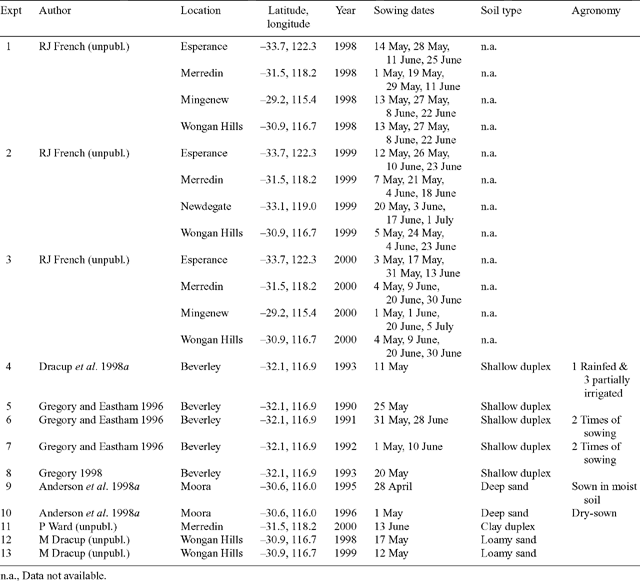
|
Measured soil characteristics and initial soil conditions were used to initialise the simulations. When soil characteristics were not available, soil types were approximated by using local soil information and one of the 5 major soil types in the cropping zone of Western Australia described by Asseng et al. (2001a). When the initial soil water content was not measured in the experiments, the soil water content of the soil profile was initialised on 1 January based on rainfall from harvest until end of previous year.
Experiments for parameter derivation
Experiments 1, 2, and 3. Observed flowering dates from several sowing dates over 3 years and 4 locations were used to derive the phenological parameters. Of the 6 narrow-leafed cultivars in the experiments, Belara (very early flowering) and Merrit (early flowering), commonly grown by farmers in Western Australia, were chosen to be parameterised. Flowering dates were defined as the dates on which 50% of the plants had at least one open flower. Physiological maturity was not recorded and so harvest date has been used as an estimate of maturity date, even though maturity often occurs well before harvest (Dracup and Kirby 1996a).
Experiment 4. This experiment was designed to investigate the variability of narrow-leafed lupin yield and harvest index caused by different levels of terminal drought. Data were used to derive model parameters that govern retranslocation and partitioning of biomass to grain. The experiment included 4 treatments, a rainfed treatment throughout the season and 3 partially irrigated treatments after flowering. The experiment was conducted in 1993 at Beverley (average annual rainfall 421 mm), WA, on a shallow duplex soil [Yellow Sodosol (Isbell 1996); USDA Typic Natrixeralf (Soil Survey Staff 1992)] with 30–40 cm of sand over-lying clay. A detailed description of the experiment is given by Dracup et al. (1998a). Soil water and N parameters needed for modelling were taken from Asseng et al. (2001a).
Experiments for model testing
Experiments 5, 6, 7, and 8. These experiments investigated the productivity and water use of a range of crops, including narrow-leafed lupin, on a shallow duplex soil at Beverley between 1990 and 1993. The soil was the same as in experiment 4. Details are published by Gregory and Eastham (1996) and Gregory (1998).
Experiments 9 and 10. Lupin phases were part of a rotation experiment conducted on a deep sand at Moora (average annual rainfall 460 mm), in the central wheatbelt of Western Australia. The soil was classified as yellow sand [Yellow-Orthic Tenosol (Isbell 1996); USDA Typic, Xeric Psamment (Soil Survey Staff 1992)]. Experimental details and results are published in Anderson et al. (1998a, 1998b) and soil parameters are given by Asseng et al. (2001a).
Experiment 11. Lupin following a canola crop was grown on a clay soil at Merredin (average annual rainfall 328 mm), a low rainfall location in Western Australia. Soil type was similar to the clay soil described by Asseng et al. (2001a).
Experiments 12 and 13. Lupin trials compared restricted-branching genotypes with a normal-branching cultivar. The experiments were conducted on a loamy sand at Wongan Hills (average annual rainfall 390 mm) in the medium rainfall zone of Western Australia. Soil type was assumed to be a loamy sand with restricted rooting depth of 150 cm described by Asseng et al. (2001a).
Model description and parameterisation
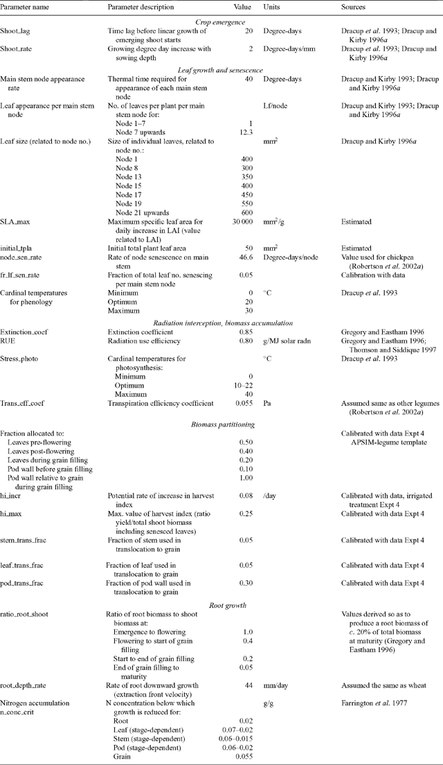
Phenology
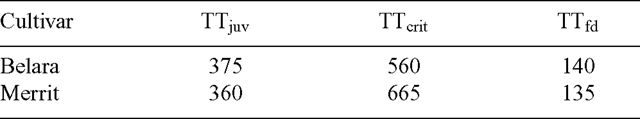
Crop phenology is simulated using a modified version of the phenology model described by Carberry et al. (1992). Thermal time is used to drive phenological development. Thermal time is calculated using 3 cardinal temperatures: base, optimum, and maximum, which were derived from published studies (Dracup and Kirby 1993, 1996a; Dracup et al. 1993) (Table 2). The phenological development of the crop to flowering is divided into four stages: (i) emergence, (ii) end of the juvenile period, (iii) floral initiation, and (iv) 50% flowering. Juvenile phase is defined as the period of development when the plant’s rate of development is not influenced by photoperiod. The duration of each period or phase is based on daily temperature and daylength. The time to flowering is a function of temperature and daylength (photoperiod). In the model, there is no response to vernalisation, as supported by the results of Reader et al. (1995). The length of the daylength-sensitive phase decreases as the daylength increases above a base daylength (PPbase) and up to a critical daylength (PPcrit). The duration of the phase depends on daylength and the daylength sensitivity (degree-days/h) of a cultivar. The thermal times at PPcrit and PPbase are termed TTcrit and TTbase, respectively. Post-flowering phases include flowering to start of grain filling, start of grain filling to end of grain filling, and end of grain filling to maturity, and are all predicted assuming fixed thermal time targets for each phase.
|
Experiments 1, 2, and 3 (Table 1), with observed dates of flowering for 4 times of sowing and locations spanning the full latitudinal range (29–34°S) over which lupin is grown in south-western Australia, were used to derive the phenology parameters up to flowering. All available experiments were used to derive parameters. We did not use the traditional calibration-validation 2-step process of model development and testing, but rather utilised all the data in the derivation of the model parameters for phenology. This approach has been used by Carberry et al. (2001) and Robertson et al. (2002b) in the development of phenology parameters for models of pigeon pea and canola, respectively. The accuracy of the prediction of time to flowering was assessed using the root mean square deviation (RMSD), which represents a mean weighted difference between predicted and observed data.
A commercial optimisation software library (NAG 1983) was used to optimise for the value of model parameters by minimising the RMSD of the number of days from sowing to flowering. After preliminary analysis of the data, PPbase and PPcrit were set to 10.8 h and 16.0 h, respectively, in order to reduce the number of parameters to be optimised. The thermal time target from end of juvenile phase to floral initiation decreases from a value TTcrit optimised at 16.0 h daylength to TTbase at 10.8 h daylength. After preliminary optimisation with no fixed parameters, TTbase was fixed to zero, so that TTcrit was the only parameter to optimise for that phase. The thermal time target from emergence to the end of the juvenile phase (TTjuv), and thermal time from flower initiation to flowering (TTfd), were also optimised (Table 3).
|
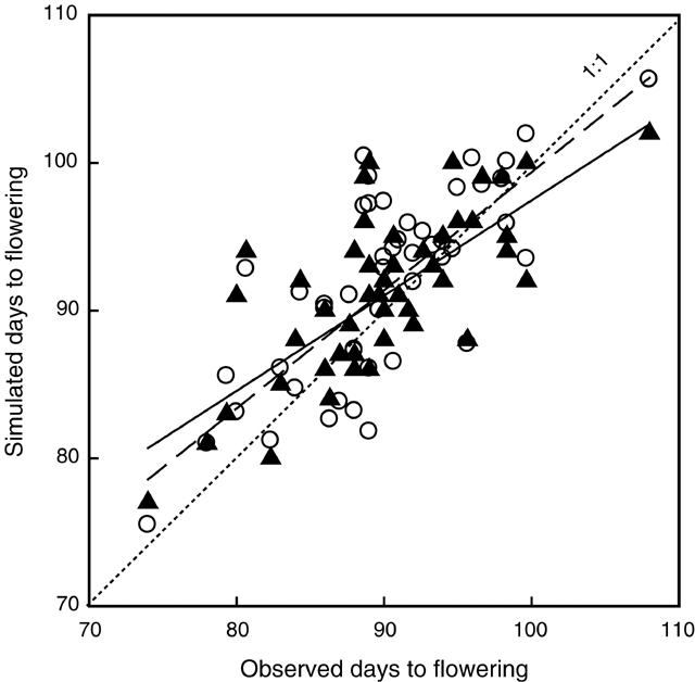
The relationship between flowering time and daylength and temperature was described for narrow-leafed cultivars by Reader et al. (1995) using multiple linear regressions. Time to flowering for a range of Western Australian lupin datasets was best explained by a model incorporating terms for average temperature and daylength between sowing and flowering. The prediction of the time to flowering by the APSIM-Lupin model was compared (Fig. 1.) with the prediction by the Reader et al. (1995) regression model.
|
The parameters for the phase between sowing and emergence were derived from published studies (Dracup et al. 1993; Dracup and Kirby 1996a) with different sowing depths and different seedbed temperatures to give a lag phase of 20 degree-days plus 2 degree-days for each mm sowing depth (Table 2).
Thermal time between flowering and the start of grain filling was derived from Expt 4. Accurate maturity data were not recorded in most of the experiments and only harvest data were available. Therefore, thermal time between start of grain filling and physiological maturity was estimated based on harvest date.
Crop development and growth
Some parameters were derived from our experimental data, whereas others were obtained from the literature (Table 2). Parameters for leaf appearance, leaf number, and leaf size were mainly taken from studies by Dracup and Kirby (1993, 1996a). These authors found that leaves appeared at a constant rate of about 40 degree-days from emergence until maturity. The study of whole-plant leaf number v. main-stem node number showed that one leaf was produced for each main-stem node produced up to node 7. After node 7, branching occurred, with 12 leaves per main-stem node produced (Table 2). Individual leaf size as a function of leaf number was obtained from Dracup and Kirby (1993, 1996a) and leaf area index (LAI) values in Expt 4.
Potential daily increase in leaf area per plant is a product of the number of leaves appearing and leaf size, which vary with node position. Actual daily increase in leaf area is less than potential if dry-matter allocation is insufficient to meet a set maximum specific leaf area for the daily increase in leaf area. Leaf senescence occurs as a function of age, light competition, drought, or frost.
Actual daily above-ground biomass increase is calculated from the minimum of a radiation- and a water-limited rate. The radiation-limited daily biomass production is calculated from LAI, a radiation extinction coefficient (K), and the radiation use efficiency (RUE) of the crop (RUE for above-ground biomass). The water-limited daily biomass is calculated from the actual soil water supply, a transpiration efficiency coefficient, and daytime vapour pressure deficit.
Parameter values and sources are tabulated in Table 2. The extinction coefficient describes the shape of the relationship between LAI and fraction of radiation intercepted. A value of K = 0.85, commonly reported (Gregory and Eastham 1996; Thomson and Siddique 1997), was used in the model. A value of RUE of 0.8 g/MJ solar radiation reported by Gregory and Eastham (1996) and Thomson and Siddique (1997) for narrow-leafed lupin cultivars was used in the model. Values of RUE ranging from 0.7 to 0.8 g/MJ solar radiation were also derived from measurements of shoot biomass and intercepted radiation for different cultivars in Expt 13 (data not shown). Values of transpiration efficiency coefficient for narrow-leafed lupin were not found in the literature and therefore assumed to be similar to other cool-season legumes (Siddique et al. 2001). A value of 0.055 Pa was used in the model.
Daily above-ground biomass production is partitioned into leaf, stem, pod, and grain according to partitioning functions that vary with developmental stage. Parameters for biomass partitioning were derived from Expt 4 and from the APSIM-Legume template. Grain demand for biomass is driven using a daily potential rate of harvest index increase (HIincr) up to a genetic maximum defined HI (HImax). A set fraction of the assimilate partitioned to grain goes to the pod-wall. If there is any assimilate available after grain demand is satisfied, the excess is used for new leaf and stem growth. The value of potential HIincr was obtained from Expt 4 by regressing HI values during the season against time. The slope of the regression for the 3 partly irrigated treatments (0.008/day) was higher than for the rainfed treatment (0.005/day). The value of 0.008/day was used as the potential HIincr in the model.
In the model, HImax (0.25) is defined as the ratio of grain yield to total above-ground biomass including senesced leaves (HIincl). Since a significant fraction of leaves is usually senesced and detached at harvest, the measured values of final biomass often overestimate HI. Therefore, simulated HI excluding senesced leaves (HIexcl) is used in comparison to observed data. Values of HIexcl can therefore be higher than 0.25.
The value for biomass remobilisation from the pod walls to the seeds (0.30) was parameterised from Expt 4 (Table 2). These values where consistent with values found in the literature (Hocking and Pate 1977; Dracup and Kirby 1996b), which resulted in simulated values for mobilisation from pod walls of around 20% of final grain yield.
Roots provide the interface between the crop and soil modules. Daily root biomass production is calculated as a proportion of the above-ground biomass, depending on developmental stage. Root depth increase is simulated using a daily potential elongation rate, which varies with crop stage. The potential elongation rate for the lupin of 44 mm/day was taken as 10% higher than in the APSIM-Wheat model. This was supported by the findings by Hamblin and Hamblin (1985), Hamblin and Tennant (1987) and Anderson et al. (1998b) who measured slightly deeper roots in lupin than in wheat in a range of soil types. However, Dracup et al. (1993) and Gregory (1998) measured similar or lower values of root depth in lupin compared with wheat in a duplex soil.
Actual root elongation is obtained from the potential elongation rate and constrained by water availability, temperature, and soil properties that limit root penetration. A root exploration factor (xf) that varies from 0 to 1 is defined for each soil layer to constrain root elongation if soil properties are known to limit root penetration. The xf factor incorporates both crop and soil factors. Values of xf for various soil types were assumed to be similar to wheat (Asseng et al. 2001a).
Water uptake is the minimum of soil water supply and crop water demand. Soil water supply is determined by soil water content above the crop lower limit in each layer occupied by roots, multiplied by a soil- and crop-specific extraction constant (kl) specified for each layer. The kl factor is empirically derived, incorporating both plant and soil factors that limit the rate of water uptake. It represents the proportion of water that can be taken up per layer per day, and values typically range between 0.10 for surface layers to 0.01 for deep layers (Dardanelli et al. 1997). Crop water demand is calculated from the potential biomass production using a crop transpiration efficiency coefficient and vapour pressure deficit.
Water stress reduces the rate of leaf expansion and RUE. The demand, uptake, and retranslocation of N are also simulated. The crop has defined minimum, critical, and maximum N concentrations for each plant part and crop stage. Demand for N attempts to maintain N concentrations at the critical level. If there is insufficient N to maintain existing and new growth at these critical levels, the rate of leaf expansion and biomass production slows. Although the focus of this work was not on N, it is an important component of the lupin module because of its role as a N-fixing legume in cropping systems.
Model evaluation
The first stage of model evaluation included testing the performance of the model on Expt 4, which was used as the base experiment for the derivation of some of the model parameters. Although this is not an independent test of the module, it is a first step in testing whether the derived parameters, when used in the module, reproduce the results of the experiments from which they are derived.
The second stage of the model evaluation process included testing the model on independent experiments. Expts 5–13 (summarised in Table 1) were used for independent evaluation of the model.
In configuring APSIM (v. 2.1) for the simulations reported in this paper, the lupin crop module was linked with the soil water module SOILWAT2, the soil nitrogen module SOILN2, and the surface residue module RESIDUE2 (Keating et al. 2003).
When available, daily climatic data were used from the Western Australian Department of Agriculture weather stations located on the experimental sites. When data were not available, they were obtained from the Australian Bureau of Meteorology through the SILO database (www.bom.gov.au/silo).
Sensitivity analysis: simulation experiment
In order to quantify the effects of variable seasonal rainfall and sowing date on yields, a simulation experiment was performed using the APSIM-Lupin model. Simulation experiments were conducted using historical long-term daily records (40 years) at two Western Australian locations, Moora, in the high rainfall zone, and Merredin, in the low rainfall zone. The soil type used in both locations is a deep sand with 55 mm plant-available water in the root-zone (Asseng et al. 2001a), typical of the northern wheatbelt of Western Australia. The soil water profile was initialised (reset) on 1 January (DOY 1) each year to the lower limit of plant-available water, assuming maximum water use in the previous crop. Previous crop residues were set each year on 1 January to 2000 kg/ha, residue type was assumed to be wheat, with a C : N ratio of 70. Soil N was reset at day of sowing each year with 50 kg mineral N/ha in the 0–70 cm depth, based on measurements in a sandy soil after a wheat crop (Anderson et al. 1998b).
Sowing time was controlled by a sowing rule. A sowing window was set between 15 April (DOY 105) and 30 June (DOY 181). The date of the first sowing opportunity occurred when at least 15 mm of rainfall had accumulated within 5 days. Two sowing date scenarios were simulated: sowing 1, sowing occurring at the first sowing opportunity every year; and sowing 2, sowing 21 days after the first sowing opportunity every year.
Results
Model parameter derivation for phenological development
The phenology model in APSIM-Lupin and the regression model developed by Reader et al. (1995) simulated similar flowering dates for a range of sowing dates and locations in Western Australia (Fig. 1). Both models tend to underestimate days to flowering for the very early sowings and overestimate it for very late sowings, even though the linear regression is not significantly different from the 1 : 1 line.
The number of days from sowing to flowering was predicted satisfactorily by the APSIM-Lupin model, across locations, years, and sowing dates. For cv. Belara (n = 38) the RMSD was 4.6 days and the R2 was 54% (data not shown). For cv. Merrit (n = 38) the RMSD was 3.8 days and the R2 was 65% (Fig. 1). The regression of simulated v. observed days to flowering was not significantly different for the 2 cultivars. The slope and the intercept were not significantly different from 1 and 0, respectively (P < 0.05).
Observed flowering dates ranged from 71 to 109 DAS and simulated values from 74 to 103 DAS. The model reproduced the flowering dates and the trend of flowering dates v. sowing date. The thermal times from emergence to end of juvenile phase (TTjuv) and from floral initiation to flowering (TTfd) were fixed (Table 3). The phase from the end of the juvenile phase to floral initiation was daylength-sensitive, with the thermal time target decreasing from the maximum value (TTcrit) for a daylength of 10.8 h to a value of zero for a daylength of 16 h. The thermal time from emergence to flowering ranged from a minimum of 515 to 1075 degree-days for Belara, and from 495 to 1160 degree-days for Merrit, depending on the daylength experienced by the crop during the daylength-sensitive phase. This was equivalent to a daylength sensitivity of 108 and 128 degree-days per hour for Belara and Merrit, respectively.
The thermal time from flowering to start of grain filling for cultivar Merrit, derived from Expt 4, was 500 degree-days. Thermal time from flowering to maturity was estimated as 1000 degree-days, based on harvest dates.
Model evaluation
Dependent testing: model performance for the experiments used to derive parameters (Expt 4)
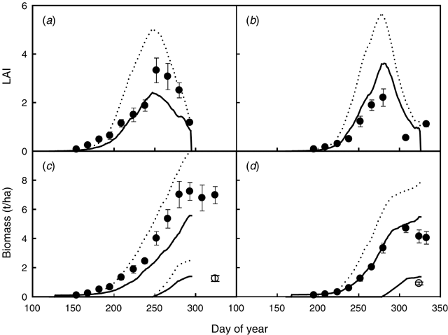
In Expt 4 (Table 1) the irrigated treatments received irrigation only after flowering. Therefore the time course of LAI for the rainfed and an irrigated treatment only differed for the period between peak LAI and final harvest (Fig. 2a, b). The model simulated accurately the increase in LAI during the first part of the season, but it underestimated the peak value of measured LAI in both treatments. The decrease in LAI after its peak was well simulated in the partially irrigated treatment but the rapid decline in LAI was underestimated in the rainfed treatment (Fig. 2a, b).
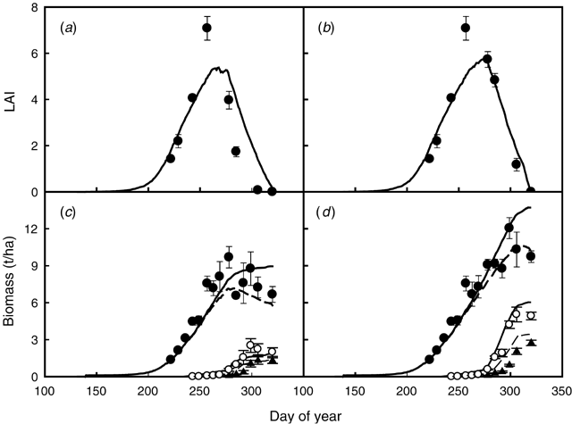
|
Observed final shoot biomass for the rainfed and irrigated treatments was 6.7 and 9.7 t/ha, respectively, and final yields were 1.3 and 2.7 t/ha, respectively. Irrigation had a greater effect in increasing yield than in increasing the shoot biomass, as shown by a measured HI of 0.20 and 0.28, in the rainfed and irrigated treatment, respectively. Much of the yield improvement with irrigation was due to extra dry matter accumulation during pod growth and a greater mobilisation of dry matter into seed (Dracup et al. 1998a). Total shoot biomass, pod biomass (pod wall + seed), and grain yield for both rainfed and irrigated treatments were well simulated by the model (Fig. 2c, d). Simulated yields for the rainfed and irrigated treatments were 1.4 and 3.4 t/ha, respectively. The effect of irrigation on shoot biomass and grain yield was well simulated by the model.
Independent testing (Experiments 5–13)
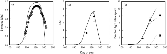
The model accurately simulated the values of light intercepted by the crop and the LAI measured in 1999 in Expt 13 (Fig. 3a, b). The rainfall amount and distribution in 1999 resulted in high biomass and final yield, which were well estimated by the model (Fig. 3c). Observed HI was 0.32 and simulated HIexcl (excluding senesced leaves) was 0.35.
|
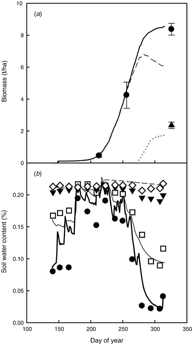
In 1993, the even rainfall distribution and the absence of waterlogging resulted in a high biomass and grain yield in Expt 8 (Fig. 4a). Even though the high grain yield was underestimated, the total above-ground biomass, and soil water content at different depths were adequately simulated by the model (Fig. 4). Most of the water uptake by the crop was in the 0–60 cm depth, with little water uptake in the 60–90 and 90–120-cm-deep layers (Fig. 4b). The pattern of water uptake was mainly due to the nature of the soil, a duplex soil with root growth constrained by a clay layer below the surface sandy layer (Gregory 1998).
|
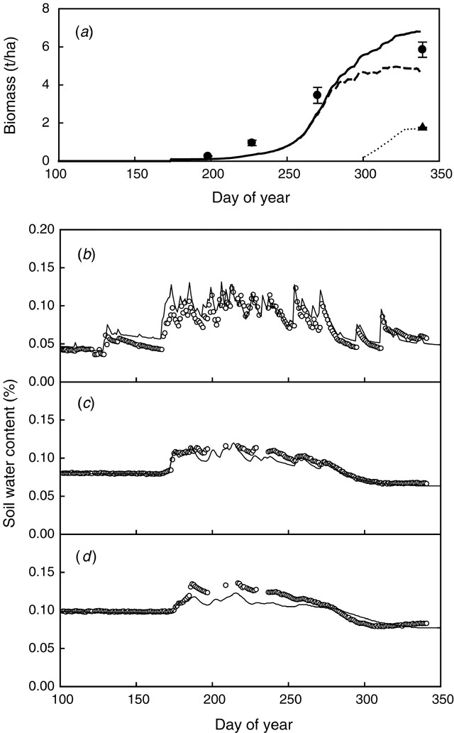
Above-ground biomass and final yield were accurately predicted for lupin grown in a deep sand in Moora in 1996 (Expt 10) (Fig. 5a). The soil water content was measured to 1.5 m depth, but root length density measurements (Anderson et al. 1998b) showed roots down to 1.8 m depth, indicating a likely water uptake from layers deeper than measured. However, soil water uptake from different layers during the season was well simulated down to the depth of the measurements (Fig. 5b, c, d).
|
The lupin crops in Expt 7 (early and late sowings) were severely affected by waterlogging, as indicated by watertable and root depth measurements taken during the growing season (data not shown). The first simulation with the APSIM-Lupin model overestimated LAI values during the season and peak LAI. Since the model did not simulate waterlogging effects, biomass and yield were also overestimated, both in the early and late sowings (Fig. 6).
|
We attempted to simulate the likely waterlogging effects on growth and yield by (1) re-creating the observed watertables and (2) testing the hypothesis of a relationship between the fraction of roots waterlogged and an oxygen stress index on RUE. We used the soil parameters derived by Asseng et al. (1998) to re-create the watertable patterns observed at this site in the 1990, 1991, and 1992 seasons. We analysed the level of sensitivity of the relationship for the oxygen stress index on RUE in order to simulate the observed shoot and yield reductions due to waterlogging at Beverley. We then parameterised the relationship for the oxygen stress factor for photosynthesis using the early sowing experiment in 1992. For values of the fraction of roots waterlogged between 0.4 and 1, the oxygen stress index decreases from 1 to 0. Model simulations accounting for waterlogging significantly improved the simulations of LAI, shoot biomass, and yield for the experiments in 1990, 1991, and 1992 in Beverley. Waterlogging effects had a small reduction in the simulated biomass and yields in the 1990 and 1991 experiments. Simulating waterlogging for 1992 caused a severe reduction on biomass and yield (Fig. 6). Those effects agree with the observation that waterlogging was more severe in 1992 than in 1991 and 1990 (Eastham and Gregory 2000). In all 3 years, the watertable appeared in mid June and persisted until mid and late August in 1990 and 1991, respectively, and until the end of September in the wetter season of 1992 (Eastham and Gregory 2000).
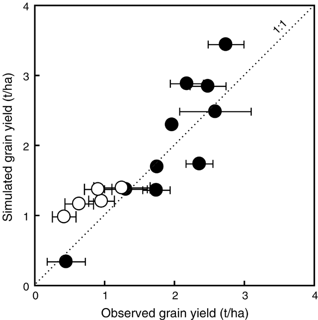
Yields from Expts 4–13 (Table 1) were included for a comparison of observed and simulated yield (n = 15) (Fig. 7). Observed yields ranged from 0.5 t/ha at Merredin (Expt 11) to 2.7 t/ha at Beverley with partial irrigation (Expt 4). Simulated yields ranged from 0.3 t/ha to 3.4 t/ha. Model simulations without accounting for waterlogging overpredicted waterlogging-affected yields at Beverley 1990, 1991, and 1992. Without waterlogging effects, yields were predicted with a RMSD of 0.6 t/ha, which was 37% of the mean of observed yield. However, when waterlogging effects were simulated by the model, the RMSD was 0.5 t/ha, being 30% of the mean of observed yields.
|
Sensitivity analysis
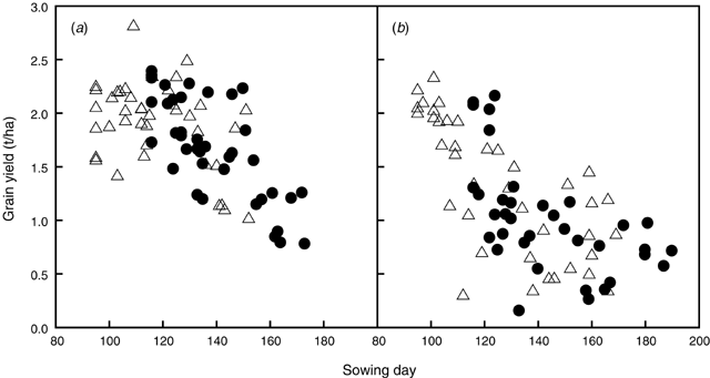
The simulation experiment allowed quantification of effects of variable seasonal rainfall and sowing date on lupin yields. These simulations did not include waterlogging effects. The sowing rule produced a range of sowing dates over the 40 years simulated, depending on dates of opening rains and rainfall patterns pre-sowing (Fig. 8). Lupin yields were highly variable because of their dependence on seasonal rainfall. In general, delay in sowing date reduced simulated yields in both locations (Fig. 8). In the high rainfall location, the delay in sowing did not reduce yields significantly for sowing dates from the beginning of April to the end of May, and yield reduction only occurred for very late sowings in June (Fig. 8a). In contrast, in the low rainfall location, any delay in sowing reduced yield (average yield reduction of 6%/week delay or 0.13 t/ha.week) (Fig. 8b). Sowing at the first sowing opportunity had an average yield advantage of 0.3 t/ha over sowing 21 days later, at both locations. This represented a 17% and 34% yield advantage in the high and low rainfall location, respectively. WUE, defined as ratio of yield (kg/ha) to April–October rainfall (mm), was higher for sowing at first opportunity (5.6–5.8) as compared with sowing 21 days later (4.0–4.4).
|
 ) and sowing 21 days later (●) in (a) Moora (high rainfall zone) and (b) Merredin (low rainfall zone), W. Aust.
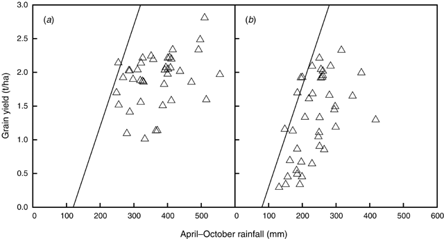
The relationship described by French and Schultz (1984) between yield and growing-season rainfall (April–October) for wheat has been widely used by farmers and advisers to estimate potential yield in Australia. The transpiration efficiency of 20 kg/ha.mm for wheat grain, which defines a ‘potential yield’, translates into 15 kg/ha.mm for lupin yield, considering the energy requirements for lupin seed (Penning de Vries et al. 1974). Siddique et al. (2001) have also reported a value of 15 kg/ha.mm as potential yield for several grain legume crops. The value for the x-intercept in the French and Schultz (1984) relationship accounted for the different seasonal rainfall patterns between locations. The intercept value used in Fig. 9 was 120 mm for Moora and 80 mm for Merredin based on Perry (1987) and using the simulated yields as a means to define an upper yield boundary.
|
Simulated lupin yields in some seasons exceeded the potential yield line. However, yields often fell below this potential line, due to uneven rainfall distribution and soils with low water-holding capacity (Fig. 9). Lupin yields were higher in the high than in the low rainfall location. In the years with higher values of April–October rainfall, particularly in the high rainfall location, grain yields fell further below the potential yield line, because a significant fraction of the rainfall was not available for transpiration as a result of deep drainage in the sandy soil (Asseng et al. 2001b). Anderson et al. (1998b) reported values of deep drainage for annual crops grown on deep sands in Western Australia in the range of 114–214 mm/year.
Discussion
An established framework used previously to simulate other grain legumes (temperate and warm-season) has been used here to develop a lupin model for inclusion as a module in the APSIM. The model demonstrated a reasonable performance for phenology, biomass, and yield across a wide range of conditions in Western Australia.
Phenology
Flowering time
In Mediterranean-type environments, where yield is often limited by terminal drought, the accuracy in simulating flowering date is particularly important. The model framework used in the APSIM-Lupin model simulated flowering date mean deviation values of c. 4 days. This deviation was close to the value of 5 days found in the APSIM-Canola model (Robertson et al. 2002b) and is also close to the deviation of 4 days in the APSIM-Wheat model (Asseng et al. 1998).
Both the phenology model in APSIM-Lupin and the regression model developed by Reader et al. (1995) simulated flowering dates for a range of sowing dates and locations in Western Australia with similar accuracy (Fig. 1). The similarity in performance of the 2 models tends to suggest that explicit accounting for a defined daylength-sensitive phase is not crucial to accurate simulation of flowering date in lupin. Despite this, the framework used in the APSIM-Lupin model allows for physiological dissection of cultivar phenology differences in response to temperature and daylength.
Both models tend to underestimate flowering date for the very early sowings and overestimate it for the very late ones. The possible existence of a small vernalisation response in modern cultivars could be responsible for the discrepancy between observed and simulated flowering day for very early sowings. The discrepancy would disappear for mid- and late-season sowings because vernalisation is satisfied quickly and the model assumption of no vernalisation response results in little error in flowering date. A possible effect of water stress on phenology could be responsible for the model overestimation for late sowings, an effect not currently accounted for in the model.
Post-flowering phenology
In lupin the duration of post-flowering phases can vary with water deficit (Dracup and Kirby 1996b). Under water stress conditions, lupin switches quickly from vegetative to reproductive mode, shortening the post-flowering phases and grain-filling period (French and Turner 1991; Dracup et al. 1998a). In Expt 4, the duration from flowering to start of grain filling was around 40 degree-days shorter in the rainfed treatment than in the partially irrigated treatments. Similarly, the grain-filling period was about 2 weeks shorter in the rainfed treatment. Changes in post-flowering phenology due to water stress are further complicated by the fact that stress enhances the rate of canopy senescence and this shortens the grain-filling period (Dracup et al. 1998a). Currently, the shortening of post-flowering phases is not simulated in the model. However, associated effects on grain filling such as the accelerating effect of water stress on leaf senescence, and the cessation of grain filling if there is no supply of assimilates, are accounted for.
Biomass growth and yield
RUE
The model showed robust simulation of total biomass and water uptake for a range of environments, indicating accuracy in the values of essential parameters such as phyllochron, K, and RUE. The low value of RUE (0.8 g/MJ) used in the model is in the range found for other temperate grain legumes [chickpea 0.69, fababean 1.15 (Turpin et al. 2002)]. Similarly, Sinclair and Muchow (1999) reported apparently low RUE values in different grain legumes. Higher RUE values have been found for warm-season grain legumes such as mungbean (0.94) and peanut (1.20) (Robertson et al. 2002a).
Partitioning/HI
Pod abortion is considered an important process influencing grain yield in lupin (Hocking and Pate 1977; Dracup et al. 1998a). However, it was possible to simulate adequate yields for a range of datasets, without accounting for the process of pod abortion in the model.
Lupin yields and harvest index are lower and more variable than in other cool-season legumes (Dracup and Kirby 1996b) and than wheat yields (ABARE 2003). The simulated HIs (0.16–0.35) were in the same range as the observed HIs (0.18–0.31). The high HI values (0.26–0.31) were well simulated by the model, whereas the low HI values (0.18–0.22) tended to be overestimated. The overestimation occurred in the low yielding experiments as a result of an underestimation of above-ground biomass, which left more water available for grain filling. The underestimation could be due to nutrient constraint associated with soil drying in spring. A similar compensation led to a reasonable simulation of grain yields despite poor simulation of the yield components in wheat (Asseng et al. 1998).
Variable and low HIs are also attributed to strong competition for assimilates between branches and pods under water-limiting conditions (Dracup and Kirby 1996b). However, the low HIs in the experiments were not correlated with high biomass crops or favourable rainfall distribution during grain filling, suggesting that the low HIs were not caused by vegetative growth at the expense of grain. The model does not simulate the competition for assimilates between vegetative parts and grain filling, but captures the main factors affecting yield and simulates yield satisfactorily over a wide range of conditions.
Yield
Yields were simulated with a deviation (RMSD = 0.5 t/ha) similar to the deviation reported for other crop simulation models (Carberry 1996). Values of RMSD of 0.4 t/ha have been reported for APSIM-Wheat (Asseng et al. 1998) and APSIM-Canola (Farré et al. 2002) in Western Australia for similar yield ranges, and RMSD of 0.5 t/ha for CERES-Wheat (Otter-Nacke et al. 1986).
Temperature. There is an indication that air temperatures of 30°C or higher during grain filling could have an effect on yield (Reader et al. 1997). This range of temperature was reached several times in the experiments used (2–14 days across datasets exceeded 30°C). However, the observed data do not suggest that yields of those experiments with high temperatures were more affected than the others. Because high temperatures coincide with increasing water deficit, it is difficult to separate their effects on yield in our experiments. In the model there is currently no additional effect of high temperatures on seed development. However, the model accounts for the major effect of water deficit on yield and gives reasonable yield predictions.
Waterlogging. Narrow-leafed lupin is very sensitive to waterlogging (Dracup et al. 1992, 1998b; Davies et al. 2000). The capability of simulating the effects of waterlogging in lupin would enable the use of the model in an exploratory way in locations and soil types where waterlogging is common, such as the agricultural region of Western Australia. Simulation of waterlogging improved the simulation of LAI, biomass, and yield. The simulations showed how the waterlogging effects on growth and yield could be captured in a simple way. In the model the only direct effect on a physiological process was via RUE. Other effects, such as on leaf expansion and N fixation, were not accounted for. Further work, incorporating a range of soil types, severities of waterlogging, and timing of waterlogging in relation to crop development is needed to establish confidence in, or further refine, the relationship used here.
Simulation experiment
The yield reductions due to delayed sowing obtained in the simulation experiment agreed with observations by Reader et al. (1995), who found that lupins are only partly able to compensate for late sowing by flowering earlier. Similarly, Eastham et al. (1999) also found that early sowing of lupin was associated with increased early growth and larger canopies resulting in higher yields. Early sowing is an important determinant of lupin yield, especially in water-limited environments, where late sowing reduces the period for biomass accumulation before a terminal drought. Similar responses have been found in wheat on sandy soils (Turner and Nicolas 1987).
The French and Schultz approach is a simple estimator for potential yield. However, it overestimates actual yields in most seasons. Hence, the simulation model can help to define the potential yield for specific rainfall zones and soil types more accurately.
Conclusions
The APSIM-Lupin model has been developed based on the APSIM-Legume template and parameterised with data from the literature and a number of experiments. The lupin model was tested for flowering date, water uptake, canopy development, biomass, and yield for 2 soil types and a range of sowing dates in Western Australia and performed well for the range of datasets under which it was tested. The model reproduced the effect of sowing date on phenology, biomass, and yield under variable growing conditions. Introducing the simulation of a waterlogging effect on RUE improved the model performance for LAI, biomass, and yield. However, a better understanding of the environmental effects on phenology, biomass partitioning, remobilisation, and yield formation would improve the capability of simulating the low and variable yields and harvest index of narrow-leafed lupins. Nevertheless, the current model can account for most of the variability due to climate, location, soil type, and management, showing that the APSIM-Legume framework used is appropriate for simulating lupin production.
The model was used to analyse the effect of variable rainfall and sowing date on yield. The model provides a tool for assessing agronomic and management options for lupin and the likely productivity of lupin in different environments and/or locations.
Acknowledgments
We thank Drs P. G. Gregory, P. Ward, G. C. Anderson and I. R. P. Fillery for providing access to unpublished data, and N. C. Turner and B. Bowden for valuable comments on the manuscript. We also thank the Department of Agriculture, Western Australia, for access to their weather station data. The research was supported by the Grains Research and Development Corporation.
ABARE (2003).
Anderson GC,
Fillery IRP,
Dolling PJ, Asseng S
(1998a) Nitrogen and water flows under pasture-wheat and lupin-wheat rotations in deep sands in Western Australia. 1. Nitrogen fixation in legumes, net N mineralisation, and utilisation of soil-derived nitrogen. Australian Journal of Agricultural Research 49, 329–343.
| Crossref |

Anderson GC,
Fillery IRP,
Dunin FX,
Dolling PJ, Asseng S
(1998b) Nitrogen and water flows under pasture–wheat and lupin–wheat rotations in deep sands in Western Australia. 2. Drainage and nitrate leaching. Australian Journal of Agricultural Research 49, 345–361.
| Crossref |
Armstrong EL,
Heenan DP,
Pate JS, Unkovich MJ
(1997) Nitrogen benefits of lupins, field pea, and chickpea to wheat production in south-eastern Australia. Australian Journal of Agricultural Research 48, 39–48.
| Crossref |
Asseng S,
Keating BA,
Fillery IRP,
Gregory PJ,
Bowden JW,
Turner NC,
Palta JA, Abrecht DG
(1998) Performance of the APSIM-wheat model in Western Australia. Field Crops Research 57, 163–179.
| Crossref | GoogleScholarGoogle Scholar |
Asseng S,
Fillery IRP,
Dunin FX,
Keating BA, Meinke H
(2001a) Potential deep drainage under wheat crops in a Mediterranean climate. I. Temporal and spatial variability. Australian Journal of Agricultural Research 52, 45–56.
| Crossref | GoogleScholarGoogle Scholar |
Asseng S,
Turner NC, Keating BA
(2001b) Analysis of water- and nitrogen-use efficiency of wheat in a Mediterranean climate. Plant and Soil 233, 127–143.
| Crossref | GoogleScholarGoogle Scholar |
Carberry PS
(1996) Assessing the opportunity for increased production of grain legumes in the farming system. Final Report to Grains Research and Development Corporation, Project CSC9 33.
Carberry PS,
Muchow RC,
Williams R,
Sturtz JD, McCown RL
(1992) A simulation model of kenaf for assisting fibre industry planning in northern Australia. I. General introduction and phenological model. Australian Journal of Agricultural Research 43, 1501–1513.
| Crossref |
Carberry PS,
Ranganathan R,
Reddy LJ,
Chauhan YS, Robertson MJ
(2001) Predicting growth and development of pigeonpea: flowering response to photoperiod. Field Crops Research 69, 151–162.
| Crossref | GoogleScholarGoogle Scholar |
Dardanelli JL,
Bachmeier OA,
Sereno R, Gil R
(1997) Rooting depth and soil water extraction patterns of different crops in a silty loam Haplustoll. Field Crops Research 54, 29–38.
| Crossref | GoogleScholarGoogle Scholar |
Davies CL,
Turner DW, Dracup M
(2000) Yellow lupin (Lupinus luteus) tolerates waterlogging better than narrow-leafed lupin (L. angustifolius). III. Comparison under field conditions. Australian Journal of Agricultural Research 51, 721–727.
| Crossref | GoogleScholarGoogle Scholar |
Dracup M,
Belford RK, Gregory PJ
(1992) Constraints to root growth of wheat and lupin crops in duplex soils. Australian Journal of Experimental Agriculture 32, 947–961.
Dracup M,
Davies C, Tapscott H
(1993) Temperature and water requirements for germination and emergence of lupin. Australian Journal of Experimental Agriculture 33, 759–766.
Dracup M, Kirby EJM
(1993) Patterns of growth and development of leaves and internodes of narrow-leafed lupin. Field Crops Research 34, 209–225.
| Crossref | GoogleScholarGoogle Scholar |
Dracup, M ,
and
Kirby, EJM (1996a).
Dracup M, Kirby EJM
(1996b) Pod and seed growth and development of narrow-leafed lupin in a water limited Mediterranean-type environment. Field Crops Research 48, 209–222.
| Crossref | GoogleScholarGoogle Scholar |
Dracup M,
Reader MA, Palta JA
(1998a) Variation in yield of narrow-leafed lupin caused by terminal drought. Australian Journal of Agricultural Research 49, 799–810.
| Crossref |
Dracup M, Turner NC, Tang C, Reader M, Palta J
(1998) Responses to abiotic stresses. ‘Lupins as crop plants: biology, production and utilization’. (Eds JS Gladstones, CA Atkins, J Hamblin)
pp. 227–262. (CAB International: Wallingford, UK)
Eastham J, Gregory PJ
(2000) Deriving empirical models of evaporation from soil beneath crops in a Mediterranean climate using microlysimetry. Australian Journal of Agricultural Research 51, 1017–1022.
| Crossref | GoogleScholarGoogle Scholar |
Eastham J,
Gregory PJ,
Williamson DR, Watson GD
(1999) The influence of early sowing of wheat and lupin crops on evapotranspiration and evaporation from the soil surface in a Mediterranean climate. Agricultural Water Management 42, 205–218.
| Crossref | GoogleScholarGoogle Scholar |
Farré I,
Robertson MJ,
Walton GH, Asseng S
(2002) Simulating phenology and yield response of canola to sowing date in Western Australia using the APSIM model. Australian Journal of Agricultural Research 53, 1155–1164.
| Crossref | GoogleScholarGoogle Scholar |
Fernández EJ,
López-Bellido L,
Fuentes M, Fernández J
(1996) LUPINMOD: A simulation model for the white lupin crop. Agricultural Systems 52, 57–82.
| Crossref | GoogleScholarGoogle Scholar |
French RJ, Schultz JE
(1984) Water use efficiency of wheat in a Mediterranean-type environment. I. The relation between yield, water use and climate. Australian Journal of Agricultural Research 35, 743–764.
| Crossref |
French RJ, Turner NC
(1991) Water deficits change dry matter partitioning and seed yield in narrow-leafed lupins (Lupinus angustifolius L.) Australian Journal of Agricultural Research 42, 471–484.
| Crossref |
Gregory PJ
(1998) Alternative crops for duplex soils: Growth and water use of some cereal, legume, and oilseed crops, and pastures. Australian Journal of Agricultural Research 49, 21–32.
| Crossref |
Gregory PJ, Eastham J
(1996) Growth of shoots and roots, and interception of radiation by wheat and lupin crops on a shallow, duplex soil in response to time of sowing. Australian Journal of Agricultural Research 47, 427–447.
| Crossref |
Hamblin A, Tennant D
(1987) Root length density and water uptake in cereals and grain legumes: How well are they correlated? Australian Journal of Agricultural Research 38, 513–527.
| Crossref |
Hamblin AP, Hamblin J
(1985) Root characteristics of some temperate legume species and varieties on deep, free-draining Entisols. Australian Journal of Agricultural Research 36, 63–72.
| Crossref |
Hocking PJ, Pate JS
(1977) Mobilization of minerals to developing seeds of legumes. Annals of Botany 41, 1259–1278.
Isbell, RF (1996).
Jones, CA ,
and
Kiniry, JR (1986).
Julier B, Huyghe C
(1993) Description and model of the architecture of four genotypes of determinate autumn-sown white lupin (Lupinus albus L.) as influenced by location, sowing date and density. Annals of Botany 72, 493–501.
| Crossref | GoogleScholarGoogle Scholar |
Keating BA,
Carberry PS,
Hammer GL,
Probert ME, Robertson MJ , et al.
(2003) An overview of APSIM, a model designed for farming systems simulation. European Journal of Agronomy 18, 267–288.
| Crossref | GoogleScholarGoogle Scholar |
Littleboy M,
Silburn DM,
Freebairn DM,
Woodruff DR,
Hammer GL, Leslie JK
(1992) Impact of soil erosion on production in cropping systems. I. Development and validation of a simulation model. Australian Journal of Soil Research 30, 757–774.
NAG (1983).
Otter-Nacke, S ,
Godwin, DC ,
and
Ritchie, JT (1986).
Penning de Vries FWT,
Brunsting AHM, Van Laar HH
(1974) Products, requirements and efficiency of biosynthesis: a quantitative approach. Journal of Theoretical Biology 45, 339–377.
| PubMed |
Perry MW
(1987) Water use efficiency of non-irrigated field crops. ‘Proceedings of the 4th Australian Agronomy Conference. Agronomy 1987 — Responding to Change’.
. (Australian Society of Agronomy: Parkville, Vic.)
Perry MW, Dracup M, Nelson P, Jarvis R, Rowland I, French RJ
(1998) Agronomy and farming systems. ‘Lupins as crop plants: biology, production and utilization’. (Eds JS Gladstones, CA Atkins, J Hamblin)
pp. 291–338. (CAB International: Wallingford, UK)
Probert ME,
Dimes JP,
Keating BA,
Dalal RC, Strong WM
(1998) APSIM’s water and nitrogen modules and simulation of the dynamics of water and nitrogen in fallow systems. Agricultural Systems 56, 1–28.
| Crossref | GoogleScholarGoogle Scholar |
Probert ME,
Keating BA,
Thompson JP, Parton WJ
(1995) Modelling water, nitrogen, and crop yield for a long-term fallow management experiment. Australian Journal of Experimental Agriculture 35, 941–950.
Reader MA,
Dracup M, Atkins CA
(1997) Transient high temperatures during seed growth in narrow-leafed lupin (Lupinus angustifolius L.). I. High temperatures reduce seed weight. Australian Journal of Agricultural Research 48, 1169–1178.
| Crossref |
Reader MA,
Dracup M, Kirby EJM
(1995) Time to flowering in narrow-leafed lupin. Australian Journal of Agricultural Research 46, 1063–1077.
| Crossref |
Reeves TG,
Ellington A, Brooke HD
(1984) Effects of lupin–wheat rotations on soil fertility, crop disease and crop yields. Australian Journal of Experimental Agriculture and Animal Husbandry 24, 595–600.
Robertson MJ,
Carberry PS,
Huth NI,
Turpin JE,
Probert ME,
Poulton PL,
Bell M,
Wright GC,
Yeates SJ, Brinsmead RB
(2002a) Simulation of growth and development of diverse legume species in APSIM. Australian Journal of Agricultural Research 53, 429–446.
| Crossref | GoogleScholarGoogle Scholar |
Robertson MJ,
Watkinson AR,
Kirkegaard JA,
Holland JF, Potter TD ,
et al
.
(2002b) Environmental and genotypic control of time to flowering in canola and Indian mustard. Australian Journal of Agricultural Research 53, 793–809.
| Crossref | GoogleScholarGoogle Scholar |
Siddique KHM,
Regan KL,
Tennant D, Thomson BD
(2001) Water use and water use efficiency of cool season grain legumes in low rainfall Mediterranean-type environments. European Journal of Agronomy 15, 267–280.
| Crossref | GoogleScholarGoogle Scholar |
Siddique KHM, Sykes J
(1997) Pulse production in Australia past, present and future. Australian Journal of Experimental Agriculture 37, 103–111.
| Crossref |
Sinclair TR, Muchow RC
(1999) Radiation use efficiency. Advances in Agronomy 65, 215–265.
Soil Survey Staff (1992).
Thomson BD, Siddique KHM
(1997) Grain legume species in low rainfall Mediterranean-type environments. II. Canopy development, radiation interception, and dry-matter production. Field Crops Research 54, 189–199.
| Crossref | GoogleScholarGoogle Scholar |
Turner NC, Nicolas ME
(1987) Drought resistance of wheat for light-textured soils in a Mediterranean climate. ‘Drought tolerance in winter cereals’. (Eds JP Srivastava, E Porceddu, E Acevedo, S Varma)
pp. 203–216. (John Wiley and Sons Ltd: New York)
Turpin JE,
Robertson MJ,
Haire C,
Bellotti WD,
Moore AD, Rose I
(2003) Simulating fababean development, growth, and yield in Australia. Australian Journal of Agricultural Research 54, 39–52.
| Crossref | GoogleScholarGoogle Scholar |
Turpin JE,
Robertson MJ,
Hillcoat NS, Herridge DF
(2002) Fababean (Vicia faba) in Australia's northern grains belt: canopy development, biomass, and nitrogen accumulation and partitioning. Australian Journal of Agricultural Research 53, 227–237.
| Crossref | GoogleScholarGoogle Scholar |