

The Characterised Noise Hi Source Finder: Detecting Hi Galaxies Using a Novel Implementation of Matched Filtering
R. JurekCSIRO Astronomy & Space Sciences, Australia Telescope National Facility, PO Box 76, Epping NSW 1710, Australia. Email: russell.jurek@csiro.au
Publications of the Astronomical Society of Australia 29(3) 251-261 https://doi.org/10.1071/AS11044
Submitted: 8 September 2011 Accepted: 8 November 2011 Published: 4 January 2012
Journal Compilation © Astronomical Society of Australia 2012
Abstract
The spectral line datacubes obtained from the Square Kilometre Array (SKA) and its precursors, such as the Australian SKA Pathfinder (ASKAP), will be sufficiently large to necessitate automated detection and parametrisation of sources. Matched filtering is widely acknowledged as the best possible method for the automated detection of sources. This paper presents the Characterised Noise Hi (cnhi) source finder, which employs a novel implementation of matched filtering. This implementation is optimised for the 3-D nature of the Hi spectral line observations of the planned Wide-field ASKAP Legacy L-band All-sky Blind surveY (WALLABY). The cnhi source finder also employs a novel sparse representation of 3-D objects, with a high compression rate, to implement the Lutz one-pass algorithm on datacubes that are too large to process in a single pass. WALLABY will use ASKAP's phenomenal 30 square degree field of view to image ~70% of the sky. It is expected that WALLABY will find 500 000 Hi galaxies out to z ~ 0.2.
Keywords: methods: data analysis — methods: statistical — radio lines: galaxies — techniques: image processing
1 Introduction
The Wide-field ASKAP Legacy L-band All-sky Blind surveY (WALLABY1; Koribalski et al. 2009, Koribalski, B., Staveley-Smith, L. et al., in preparation) is an ambitious project that aims to detect neutral hydrogen to a redshift of z ~ 0.26, across ~70% of the sky. It is one of the two top-ranked projects that will be carried out using the Australian SKA Pathfinder (ASKAP). WALLABY is possible because of ASKAP's unprecedented ~30 sq. degree field of view, which is achieved using Phased Array Feeds (PAFs). WALLABY will use all 36 of ASKAP's antennae, but due to limitations on computing resources will only process the inner 30 antennae (with a maximum baseline of 2 km) to image the sky with a 30″ synthesised beam and produce datacubes with voxels2 that project to ~10″ on the sky. The high spatial resolution is complemented by an anticipated spectral resolution of 3.86 km s–1. ASKAP spectral datacubes will therefore cover a large area of the sky to high resolution, which results in very large datacubes containing at least 2048 × 2048 × 16 384 voxels. WALLABY will consist of ~1200 of these large datacubes. The size and number of these datacubes renders manual source finding unfeasible. The performance of the automatic source finder used by WALLABY will determine how many (Hi) galaxies are found by WALLABY.
The majority of source finders in existence use intensity thresholding to find sources. sextractor (Bertin & Arnouts 1996), sfind (Hopkins et al. 2002) and duchamp (Whiting 2008, 2011) are good examples of source finders based on intensity thresholding. Conceptually, intensity-threshold source finders check every pixel (voxel) in an image (datacube) to see if the pixel (voxel) value is sufficiently extreme that it's unlikely to be noise. Once all of the source pixels (voxels) have been identified, they are combined into objects. The various intensity threshold source finders differ in how they estimate the noise, set a threshold for identifying source pixels (voxels), pre-process the image (datacube) to improve the source finder results and the manner in which they create objects from source pixels (voxels). All intensity threshold source finders share an inherent limitation, though.
Consider an arbitrary source in a spectral datacube. Improved spatial and spectral resolutions result in the source occupying more voxels in the datacube. Dispersing the source's signal over more voxels means that it contributes less to the flux value of each voxel that it occupies. This makes it harder for an intensity threshold method to detect the source. Using a simple model this effect is illustrated in Figure 1, where the maximum voxel S/N of an object with an integrated S/N of 5 is plotted for various asymmetries. The maximum voxel S/N is calculated to be  , where β describes the asymmetry of the object's flux distribution and n is the number of voxels.
|
By overlaying the minimum expected size (in voxels) of WALLABY sources on Figure 1, we can assess the impact of this inherent limitation on WALLABY. The neutral hydrogen detected in emission is warm, which gives it an intrinsic amount of dispersion. We will assume that any real WALLABY source extends over at least 3 channels. We will also assume that in every channel, a source occupies at least 3 × 3 voxels for a 30″ synthesised beam and 10″ voxels). Galaxies rarely lie at the middle of a voxel, though, so a more realistic minimum is a grid of 4 × 4 or 5 × 5 voxels in every channel. It is expected that most galaxies detected by WALLABY will be unresolved or at most marginally resolved (Duffy, A., Meyer, M. & Staveley-Smith, L. 2011, in preparation), so we also consider a 7 × 7 grid of voxels in every channel to account for marginally resolved, off-centre galaxies. After multiplying by the minimum number of channels to obtain the expected minimum size of WALLABY galaxies in voxels, the minimum size for these different grids is overlaid in Figure 1. This demonstrates that off-centre and/or marginally resolved galaxies will be difficult to detect with a basic implementation of an intensity-thresholding source finder, unless the flux is asymmetrically distributed. Figure 1 also illustrates that this effect is amplified in 3-D datasets such as future WALLABY datacubes. For example, in a 2-D image the 7 × 7 and 5 × 5 vertical lines would approximately lie at the position of the 4 × 4 and 3 × 3 vertical lines.
This inherent limitation is compounded further by using a size-based rejection criterion to weed out false detections. If you only detect a few unconnected voxels, the source will be flagged as a false positive by a size-based rejection criterion. Off-centre and/or marginally resolved galaxies that are detected because of asymmetric flux distributions are most likely to be detected in the form of a few unconnected voxels. This effect will also show up as an enhanced fracture rate of extended, well-resolved sources.
The inherent limitation of intensity thresholding–based source finders can be offset by using more aggressive intensity thresholds (i.e., lower intensity thresholds), but this often results in many false (source) detections. The solution to this problem is to run the source finder on the datacube multiple times with the datacube smoothed to a different scale each time. This is however a very inefficient solution to the problem. duchamp provides multiple options for dealing with this inherent limitation: a secondary ‘growth’ threshold, smoothing and a 3-dimensional wavelet reconstruction of the dataset.
As part of its design study, WALLABY has investigated novel methods of source detection as an alternative to multiple passes of an intensity threshold source finder. The goal of this investigation was to develop source detection methods that are optimised for large datacubes with high spatial and spectral resolution. The Characterised Noise Hi (cnhi) source finder that I present here is one of the novel source detection methods that have been developed.
The rest of the paper is structured as follows. The conceptual framework for the cnhi source finder is presented in Section 2. The inherent limitations of the cnhi source finder are then discussed in Section 3. Next, the current implementation of the cnhi source finder is presented in Section 4. Finally, some example results are discussed in Section 5 before finishing with a summary.
2 Conceptual Framework
The cnhi source finder is based on three concepts. The first concept is that WALLABY spectral datacubes can be treated as bundles of Hi spectra, rather than collections of voxels. The next concept is that contiguous blocks of voxels should be tested to see if they're a source, rather than individual voxels. The final concept is that a ‘source’ is detected by looking for a region in a datacube that doesn't look like noise. This is the inverse of most source finders, which identify sources based on some idea of what a source looks like. In the rest of this section these concepts are explained in detail.
The first part of the cnhi source finder conceptual framework is treating a WALLABY spectral datacube as a bundle of Hi spectra, which is akin to Integral Field Unit (IFU) observations. Each position on the sky has its own spectrum. However, each spectrum in this datacube is correlated to some degree with the neighbouring spectra. The ASKAP beam will determine the degree of correlation between each spectrum and its neighbouring spectra. As explained later the correlation between spectra should not be a problem for the cnhi source finder. This conceptual view of a WALLABY datacube is very amenable to parallelisation.
The second component of the cnhi source finder conceptual framework is to test contiguous blocks of voxels instead of individual voxels. This concept is designed to take advantage of WALLABY datacubes having sufficiently high velocity resolution to reasonably resolve most galaxies in frequency. As discussed above, high resolution data is problematic for source finding methods that analyse individual voxels. The high resolution is, however, advantageous when testing contiguous blocks of voxels. A single voxel with a flux value that is one standard deviation above the mean is not significant. Ten contiguous voxels that are all one standard deviation above the mean are, because it's improbable that this will happen by chance in a spectrum with negligible correlation. If we can test whether a contiguous block of voxels in a spectrum is likely to be source, then we are searching for sources in a way that benefits from the high velocity resolution of WALLABY datacubes.
Testing whether contiguous blocks of voxels are sources provides additional information compared to testing individual voxels. It is a reasonable expectation that the test region that best fits the position and velocity width of a source in a given Hi spectrum is the most significant test region. If the test region is too small, then it should be less significant than a larger region that is also made up of source voxels. If the test region is too large, then the test region contains both source and pure noise voxels, which should result in a less-significant test region. Identifying the position and width that results in the most significant test region therefore provides an estimate of the source position and velocity width.
The final concept of the cnhi source finder is to find sources by looking for regions in a WALLABY datacube that do not look like noise. Looking for regions that do not look like noise is a novel way to implement matched filtering. Rather than using many, many filters that each describe a different type of source, we can use a single filter that looks like noise. This works because we can safely assume that the presence of a source is what causes a contiguous region in our datacube to not look like noise. The key is to use the noise distribution as the filter, because it is relatively stable, even though individual realisations of the noise vary.
How do we use the noise distribution as a filter to look for regions that aren't pure noise? Due to the large size and high resolution of WALLABY datacubes they are expected to be sparsely populated by sources. This means that an arbitrary Hi spectrum will be dominated by noise. If we select a test region of contiguous voxels, then we can use the rest of the Hi spectrum as an example of noise. A comparative statistical test such as the Kolmogorov–Smirnov test (Kendall & Stuart 1979) can then determine the probability that the test region and the rest of the spectrum, which is noise dominated, come from the same distribution of voxel fluxes. In other words, using a comparative statistical test we can identify whether a test region looks like noise. This implementation can easily be adapted to 2-D images and spectra.
The cnhi source finder uses the Kuiper test (Kuiper 1960) to compare the voxel flux distribution of a test region to the rest of the spectrum, and identify regions with non-noise voxel flux distributions. The Kuiper test is a variant of the Kolmogorov–Smirnov test that is cyclically invariant. The Kolmogorov–Smirnov test is most sensitive to differences in the distributions about the medians of the distributions. The Kuiper test by contrast is equally sensitive to differences in the two distributions throughout their entire range.
3 Inherent Limitations
There are two inherent limitations of the cnhi source finder. These limitations are tied to the conceptual framework. The first limitation is that the comparison of the test region with the rest of the Hi spectrum relies on a noise-dominated Hi spectrum. The other limitation is that a test region needs to be sufficiently large for the Kuiper test to produce reliable results.
The use of the Kuiper test to determine whether a region in an Hi spectrum is noise-like is predicated upon the assumption that the voxel flux values of the rest of the Hi spectrum are noise. It is expected that the assumption of noise-dominated Hi spectra is valid for properly calibrated, flagged and continuum-subtracted WALLABY datacubes with no significant baseline structure. To illustrate the sparsity of WALLABY datacubes, a typical WALLABY datacube is only 0.6% source (measured in voxels), if 500 000 sources distributed across 1200 datacubes have a typical size of 1 000 000 voxels.
For datacubes that are not well behaved or sufficiently sparse (e.g., baseline structure or failed bandpass calibration), this can be dealt with by comparing a test region in an Hi spectrum to the subset of the remaining Hi spectrum in its immediate vicinity. The Kuiper test will be less sensitive, but this is offset by making a valid statistical comparison. Fourier analysis, polynomial fitting and existing baseline structure–removal techniques (such as those implemented in duchamp) can also be used in combination with this approach, or as an alternative.
The validity of a Kuiper test is described by the Q parameter. For two samples containing n1 and n2 values, the Q parameter is n1 × n2/(n1 + n2). This is the same Q parameter that describes the validity of the Kolmogorov–Smirnov test. For both the Kuiper and Kolmogorov–Smirnov tests it is accepted that the test results are valid for Q ≥ 4. The test region in an Hi spectrum needs to be sufficiently large to satisfy Q ≥ 4, otherwise the Kuiper test results are increasingly spurious for increasingly smaller test regions. Setting n = n1 + n2, Q = 4 and letting m be the minimum size of a test region, then we can solve for m. The minimum size of a test region is  .
.
For a WALLABY datacube the minimum size of a test region is 4 channels. This matches the minimum expected channel width of WALLABY Hi galaxies. The use of the cnhi source finder on other datacubes needs to consider the minimum size of a test region. For reference the minimum test region size is 4 channels for n ≥ 40, and the Kuiper test cannot achieve Q ≥ 4 for n ≤ 15.
4 Current Implementation
The current implementation of the cnhi source finder works in the following manner. A user calls the cnhi source finder from the command line with a list of input parameters. The software then figures out how many chunks to split the input file into, such that each chunk is at most 1 GB in size. For each chunk, the software creates a bundled Hi spectrum for each position on the sky and uses the Kuiper test to find object sections in the bundled spectrum. Once all of the bundled Hi spectra have been searched for object sections, the software creates objects out of them using a variant of the Lutz one-pass algorithm (Lutz 1980). The list of objects, their properties and postage-stamp images are external to the chunks and new objects are added as each chunk is processed. Once all of the chunks have been processed, the final list of objects is tested against the user-specified rejection criterion. The objects that remain are then output to a catalogue, added to global moment 0 and position–velocity plots and postage-stamp images (including integrated spectra) generated. A flow diagram of the current implementation is presented in Figure 2. The following subsections provide more detail about the cnhi input and output, the bundling of multiple Hi spectra, finding object sections in a bundled Hi spectrum and the creation of objects from object sections.

|
4.1 Inputs and Outputs
User input consists of the following parameters:
-
Output code: The output catalogue and plots are created with names of OutputCode_obj.cat, OutputCode_plots and OutputCode_spectra.
-
File name: The path to and name of the .fits file that cnhi will search for sources.
-
Pre-threshold: The probability threshold used to identify interesting regions that are likely to contain a source.3 (Dimensionless quantity.)
-
Threshold: The probability threshold used to identify sources within interesting regions.3 (Dimensionless quantity.)
-
Minimum bounding box (3 values): The size criterion applied to an object's bounding box if it is to be retained.
-
Bounding box filling factor: An object composed of fewer voxels than the minimum bounding box multiplied by the filling factor is rejected.
-
Pseudo total intensity threshold: Objects with a pseudo total intensity less than this threshold are rejected.
-
Merging distances (3 values): Objects which are separated by this many voxels or fewer in any dimension are merged into a single object.
-
Maximum scale: The maximum size of a test region in an Hi spectrum. Specified in number of channels.
The cnhi source finder output consists of a catalogue, a global moment 0 map, a global position–velocity diagram for both RA and Dec, and postage-stamp images of each object (including an integrated spectrum). The cnhi source finder catalogue contains the following information for each object:
-
ID: A numerical ID assigned to each object.
-
Voxel count: The number of voxels that constitute the source.
-
Pixel RA: The mean RA of the object's voxels.
-
Pixel Dec: The mean Dec of the object's voxels.
-
Pixel channel: The mean channel of the object's voxels.
-
Intensity RA: The flux-weighted mean RA of the object's voxels.
-
Intensity Dec: The flux-weighted mean Dec of the object's voxels.
-
Intensity channel: The flux-weighted mean channel of the object's voxels.
-
Voxel limits (6 values): The minimum and maximum RA, Dec and channel of the object.
-
Voxel flux statistics (5 values): The sum, mean, minimum, maximum and standard deviation of the object's voxel flux values.
-
Two sets of W20 and W50 measurements.
-
Sparse representation: A sequence of values that describes a sparse representation of the object's 3-D bit mask in the datacube's voxel co-ordinates.
The W20 and W50 measurements are measured in two ways. The first set of W20 and W50 measurements uses the same method as duchamp. First, the global maximum of the object's integrated spectrum is determined. Next, starting from each end of the integrated spectrum the first channels with a flux greater than or equal to 20% and 50% of the maximum are identified and used to measure W20 and W50. The second set of width measurements was developed as part of the source finder framework that is used to implement cnhi. First, the total flux of the integrated spectrum is measured. The cumulative frequency distribution (cfd) of the total flux is then constructed as a function of channel number for the integrated spectrum. The inner 92.7% and 76.1%, which correspond to the conventional W20 & W50 for a Gaussian profile, are then used to determine W20 and W50. The cfd will oscillate at the edges of the integrated spectrum because of noise. For this reason the ‘inner’ values are defined (starting from the left edge of the integrated spectrum) to start at the channels where the cfd never again dips below 0.0364 (W20) and 0.1195 (W50), and ends at the channels where the cfd first rises above 0.9636 (W20) and 0.8805 (W50). This approach to measuring W20 and W50 has a consistent physical meaning across all possible spectral profiles and ‘in principle’ averages out noise.
4.2 Creating Bundled Hi Spectra
For each Hi spectrum the cnhi source finder bundles together this Hi spectrum and the neighbouring Hi spectra. This bundled Hi spectrum is searched for objects. A bundled spectrum is created by weighting the sum of the Hi spectrum and its neighbouring Hi spectra using the point spread function.
Searching for object sections in a bundled spectrum has two advantages. The first advantage is that it slightly improves the S/N without blurring the edges of sources in velocity space or creating correlation in the bundled Hi spectrum. The second, more important advantage is the improved detection of the outer edges of a source. Bundling the Hi spectra couples the brighter flux in an object's inner region to the fainter flux at the edge of the object. This improves the chance of detecting the fainter outer regions of the object. The amount of improvement varies nonlinearly with source morphology, user input and datacube, so no attempt is made here to predict the amount of improvement.
4.3 Finding Object Sections
The Kuiper test is used to find object sections within a bundled Hi spectrum. This is implemented as a four-step process. In the first step, the Kuiper test is used to identify interesting regions that are likely to contain an object section. The next step is to reduce the list of interesting regions to a unique set. This is achieved by finding all of the interesting regions that overlap, and only keeping the most significant interesting region. The most significant interesting region is judged to be the region with the lowest probability of being noise according to the Kuiper test. The purpose of these first two steps is to efficiently reduce the bundled spectrum to a manageable subset. Third, the Kuiper test is applied to every position on every relevant scale to find object sections within these interesting regions. The final step is to reduce the object sections to a unique set. This is achieved in the same way that interesting regions are reduced to a unique set.
Interesting regions are found by applying the Kuiper test to test regions in the bundled Hi spectrum and comparing the result to a user-defined pre-threshold. Interesting regions are found efficiently by Nyquist sampling both the scales of interest and positions along the bundled Hi spectrum. Starting with the largest scale of interest (user-specified) and the beginning of the bundled Hi spectrum, the Kuiper test is applied and then the test region is advanced half of the scale length. Once the entire bundled spectrum has been tested on this scale, the scale is halved and the process is repeated. This is repeated until the minimum scale has been processed.
Interesting regions narrow down the location and scale of object sections. Only positions within the interesting region, and scales ranging from half as small as the interesting region up to the size of the interesting region, need to be investigated. If other positions or scales were a better fit for object sections located within this interesting region, then this wouldn't be the most significant interesting region. The Kuiper test is applied to all possible combinations of position and scale efficiently using a test region that expands and then shrinks as it moves to different positions.
4.4 Creating Objects from Object Sections
Once the cnhi source finder has finished finding object sections in a chunk of the datacube, the object sections are combined into objects. Objects are created from object sections using a variant of the Lutz one-pass algorithm. The essence of the Lutz one-pass algorithm is to raster scan through an image or datacube, building up the properties of every object as you go. Lutz's crucial insight is that objects are simply connected so they pop out of the current image or datacube section being scanned (the scanline). This places a limit on the number of objects that need to be tracked and updated at any one time. Once the entire datacube is scanned, the rejection critierion is applied to the objects. The surviving objects are written to the output catalogue.
The crucial change to the Lutz one-pass algorithm is the use of sparse representations of 3-D objects. The use of sparse representations is what allows the cnhi source finder to process the datacube in chunks. A new sparse representation, which consists of three components, was developed expressly for this purpose. The first component lists the RA and Dec widths of the object's bounding box. The second component lists the number of object sections that make up the object prior to a given RA, Dec position. The final component lists the channels that each object section begins and ends at. The first component indexes the second component, which then indexes the third component. The structure of this sparse representation is illustrated in Figure 3.
|
The flaw of the Lutz one-pass algorithm is that it assumes objects are never encountered again after they ‘pop’ out of the scanline. This assumption is quite easily invalidated when a datacube is too big to process in a single pass. A crude solution is to split the datacube into overlapping chunks, process them individually and then merge the detections within the chunk overlaps. This approach can easily produce erroneous result, because it relies on the positions of a source's segments being sufficiently close to be merged together. A better method is to update each chunk's mask with all of the previously detected sources before processing them. To do this we need to be able to efficiently store the binary mask of every object in a readily accessible format. The sparse representation of 3-D objects presented here enables the cnhi source finder to do exactly that. This approach to processing arbitrarily large datacubes also makes the cnhi source finder readily amenable to distributed/parallel computing.
An additional benefit of using the sparse representations is that the binary mask of every object can be written to the cnhi output catalogue. Storing an object's binary mask allows us to run an arbitrary source parametrisation tool without having to re-run the source finder to generate the binary mask.
The cnhi source finder incorporates the sparse representation of 3-D objects in the following way. The flag array, which stores the object sections found in the datacube chunk currently being processed, is first updated for the objects found in previous chunks using their sparse representations. The cnhi source finder then scans through the flag array until it finds a voxel that has been flagged as source. The software then searches through the flag array to find previously processed objects within the voxel's user-specified merging volume. This is a 3-D implementation of what is referred to as 8-connected linking in 2-D images. If there aren't any objects within the merging volume, then a new object and sparse representation is created. If a single existing object is found within the merging volume, then the source voxel is added to it. If multiple existing objects are found, then the existing objects are merged into a single object and the source voxel added to it. In each scenario the flag array is updated with the object ID of the source that each source voxel belongs to. When existing objects pass out of the merging volume of all possible new objects, the user-specified rejection criterion is applied to these existing objects. This ensures the minimal number of objects is stored in memory at any given time. The object IDs of rejected objects and the memory used to store their properties and sparse representations are recycled. After the flag array has been scanned, the sparse representations and postage-stamp images of the surviving objects are constructed/updated as required.
5 Example Results
An analysis of the completeness and reliability of the cnhi source finder, and a comparison of its performance to other source finders, is presented in Popping et al. (2012). This paper presents a complementary analysis to that of Popping et al. (2012), using the same point source (PS) and extended source (ES) test datacubes (Westmeier et al. 2012). The terms ‘completeness’, ‘raw reliability’, ‘refined reliability’, ‘merging rate’ and ‘fragmentation rate’ are defined and measured as in Popping et al. (2012). As in Popping et al. (2012) and Westmeier et al. (2012), the analysis presented here acknowledges the difference between ‘raw reliability’ and ‘refined reliability’, the ‘refined reliability’ being the reliability that it is possible using post-processing to remove false detections from a source finder's output catalogue. From here on, the term ‘reliability’ will refer to the raw reliability. Note that the refined reliability has a corresponding refined completeness, which accounts for the true detections that are incorrectly flagged as false detections during post-processing.
During visual inspection of the cnhi source finder detections in various parameter spaces, it was discovered that the total intensity versus maximum voxel intensity (intensity of the source's brightest voxel) parameter space is the most efficient parameter space in which to post-process cnhi detections. For a given object with a given total intensity, the more compact it is, the brighter the maximum voxel intensity. For each threshold a simple cut (a line) in this parameter space was used to post-process the cnhi detections. The line was adjusted for each threshold until the refined reliability was greater than 90%. This required minimal effort, and is an example of the type of post-processing advocated in Serra et al. (2012).
The completeness, reliability, refined completeness and refined reliability are plotted in Figures 4 and 5 for the PS and ES datacubes as a function of threshold. In Figure 4, the inherent limitation of the cnhi source finder is taken into account by measuring a ‘corrected completeness’. The corrected completeness is measured by excluding sources in the PS input catalogue with a full-width at half-maximum smaller than four channels. This corrected completeness therefore measures the completeness of the sources that the cnhi is expected to find. The refined completeness in Figure 4 is that of the corrected completeness. The inherent limitation of the cnhi is only taken into account for the PS datacube, because a significant fraction of the sources in the PS datacube have Gaussian profiles with FWHMs that extend over 3 channels or less. Uncertainties are not provided for the curves in Figures 4 and 5, because to generate meaningful uncertainties requires generating many noise realisations. This is beyond the scope of this paper. It is also irrelevant, because the performance of the cnhi source finder on the PS and ES datacubes is not a guarantee or guide to the performance of the cnhi source finder on other datasets.
|
|
As expected, when generating the curves in Figures 4 and 5, the choice of pre-threshold has as much of an impact on the completeness as the choice of threshold. To obtain the best completeness the pre-threshold should be set as high as computer resources and the datacube size will allow. Note that it was also observed that a pre-threshold larger than 0.1 or even 0.01 is excessive, and needlessly computationally expensive. Pre-thresholds larger than 0.1 or 0.01 are unlikely to improve upon the number of real sources that are recovered. For this reason a pre-threshold of 0.01 was used to generate Figures 4 and 5.
The curves in Figures 4 and 5 illustrate that it is possible to achieve a good combination of refined completeness and refined reliability. For the PS dataset it was possible to achieve a refined, corrected completeness of ~80% with a refined reliability of ~95%. A refined completeness of ~50% was achieved for the ES datacube, also with a refined reliability of ~95%. For both datasets the curves in Figures 4 and 5 have negligible merging and fracture rates.
Thresholds of 10–3 and 10–6 produce arguably the optimal combination of refined completeness and refined reliability in Figures 4 and 5. For this reason, the performance of the cnhi source finder when using these thresholds was examined further. First, the completeness was measured as a function of maximum voxel flux. Next, the fraction of total flux recovered by the cnhi source finder was measured as a function of source total flux. Finally, the distribution of the difference between the true position of the sources and the position measured by the cnhi source finder was determined.
Figure 6 shows that the cnhi source finder can find almost all of the PS objects with a maximum voxel intensity five times brighter than the noise, with a high refined reliability. The cnhi source finder also finds a significant fraction of PS objects with a maximum voxel intensity between three and five times the noise. Unfortunately, the cnhi source finder does not perform as well at finding the ES objects. Visual inspection of the undetected ES objects revealed that they are ‘pancake’ galaxies. These pancake galaxies are spatially resolved, but due to orientation only extend over a few channels. The bundling of Hi spectra acts as a crude spatial filter, and the bundling used here closely matches the spatial profile of the PS objects. This suggests that the cnhi source finder can be improved by using multiple bundling schemes. This improvement would be equivalent to using matched filtering in three dimensions, with the spatial and frequency dimensions using independent filters.
|
The fraction of each source's total intensity that is recovered by the source finder is plotted in Figure 7, and is referred to as the recovery fraction. The mean recovery fraction is measured after excluding fragmented sources, and is overlaid in Figure 7. A poor recovery fraction requires post-processing of each detection by a second tool to improve the source parametrisation. The mean recovery fraction for the 10–3 threshold in Figure 7 asymptotes from ~80% to ~90% as sources become brighter. The recovery fractions greater than 100% are a result of comparing total intensities measured in the noisy datacube to a reference total intensity measured in the noise-free datacube. This is the most meaningful comparison, though, because it is sensitive to object masks that are either too large or too small. The recovery rate is as good as I would expect to do, without overestimating the total flux. This demonstrates that minimal post-processing is required to improve the parametrisation of sources detected by the cnhi source finder.

|
Using more conservative thresholds of 10–5 and 10–7, which do not push as far into the noise as higher thresholds,4 results in a median recovery fraction that asymptotes from ~50% to ~90% and ~50% to ~70% as sources become brighter. The median recovery fraction appears to asymptote more rapidly for more aggressive thresholds. This suggests that as the choice of threshold becomes more aggressive, the total flux measured for a source will converge to its true value. This suggests two things. First, the sources with low recovery fractions in the left panel of Figure 7 are probably objects that have only barely been detected, and using a more aggressive threshold would result in a higher recovery fraction. Second, an alternative use of the cnhi source finder is as a source parametrisation tool rather than a source finder.
The final component of the analysis is the distribution of the separation in voxels between the centre of the sources and their corresponding detection. The separation distributions of the voxel centres and intensity-weighted voxel centres are presented in Figure 8.
|
A separation between the centre of an object and its corresponding cnhi detection reveals biased source detection. The centres of an object and its corresponding detection are calculated as an unweighted mean of the voxel positions or a flux-weighted mean of the voxel positions. It can be safely assumed that the voxel and weighted voxel centres of an object are accurate. A non-zero separation therefore arises due to a distorted source detection, where one region of the source is detected more than the rest. If the mean voxel centre separation is sharply peaked about a separation of zero, then we can conclude that cnhi detections are on average unbiased representations of the corresponding source. If the mean weighted voxel centre separation is similarly distributed, this demonstrates that the cnhi detections are on average an unbiased representation of the source's flux distribution. In Figure 8 the unweighted (intensity-weighted) separation distributions of both the PS and ES datasets are sharply peaked at 0.7 (0.3) and 0.9 (0.5) voxels. This demonstrates that the cnhi source finder detections are typically a fair, unbiased representation of the underlying source and its flux distribution.
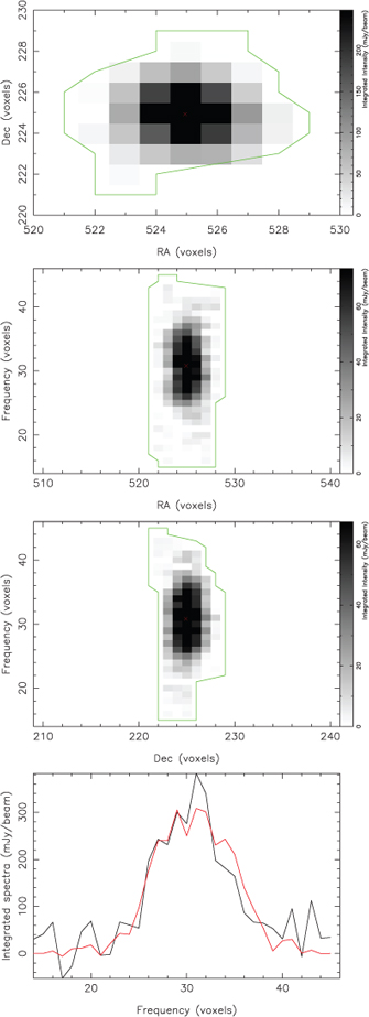
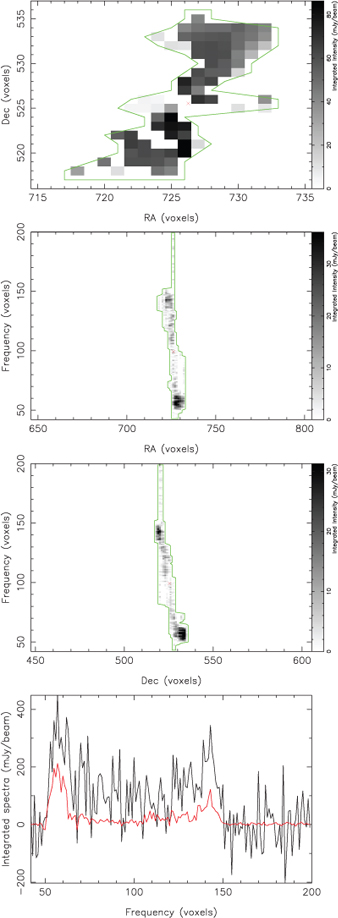
This section finishes by presenting examples of the postage-stamp images generated by the cnhi source finder. Figures 9 and 10 are postage-stamp images for two objects selected at random from the PS and ES dataset (one from each dataset). Both figures demonstrate the ability of the cnhi source finder to find the boundaries of sources. Figure 10 also nicely illustrates that the cnhi source finder is capable of detecting an object extending over many channels as a single object, rather than fragmenting it into two or more detections.
|
|
6 Summary
WALLABY and other projects that will be carried out on the next-generation radio telescopes ASKAP and MeerKAT herald the start of the data-deluge era in radio astronomy. The sheer size of WALLABY datacubes necessitates automation of many tasks in the data reduction pipeline that previously would have been carried out with some level of manual input by an astronomer. Complete automation of finding Hi galaxies in spectral datacubes is one of the challenges that is actively being investigated by WALLABY.
The resolution and size of WALLABY observations poses a challenge for many existing automated source finders. This challenge arises from the underlying conceptual framework and algorithm that these source finders are based on, and not a flaw in the implementation. The cnhi source finder has been developed using a conceptual framework that can handle the large size of WALLABY datacubes and takes advantage of the resolution. Treating a datacube as a set of spectra (akin to an IFU observation), it attempts to find sources by looking for regions in each spectrum that do not look like noise. This is achieved using a novel implementation of matched filtering. Instead of using multiple filters that describe various types of sources, a single filter describing the noise is used. Sources are detected using this noise filter by identifying regions that do not look like noise.
The performance of the cnhi source finder was tested using the PS and ES datasets in Westmeier et al. (2012). Analysis of the cnhi source finder output demonstrated that a reasonable combination of completeness and refined reliability can be achieved. A refined completeness of ~80% and ~50% was achieved for the PS and ES datasets, respectively, with a refined reliability of ~95%. The PS dataset is better than the 80% completeness would suggest, though, because the cnhi source finder found ~95% of all PS objects with a maximum voxel flux ≥5σ, with a refined reliability of ~95%. This analysis also demonstrated that the cnhi source finder recovers a significant fraction of the source flux. The recovery fraction asymptotes towards 100% as the total flux increases. More aggressive (larger) thresholds result in a recovery fraction that asymptotes faster, and starts higher. This suggests an alternative use of the cnhi source finder as a source parametrisation tool used in tandem with another source finder. Finally, the performance analysis demonstrated that cnhi detections of a source are an unbiased representation of the source and its flux distribution. These results are very promising, and warrant further testing and refinement of the cnhi source finder.
There are three development goals for the cnhi source finder. Further development of the cnhi source finder will initially focus on incorporating multi-scale bundling. This will effectively achieve independently scaled matched filtering in both the frequency and spatial dimensions. Additionally, the cnhi source finder will have a simple intensity thresholding test added to it. Incorporating an intensity thresholding test will make the cnhi source finder sensitive to sources occupying 3 or fewer channels. The final development goal is to incorporate Fourier analysis, polynomial fitting and existing baseline structure–removal techniques. Upon completing this next development cycle, the cnhi source finder will be tested and tweaked using the next round of ASKAP simulations and the Hi Parkes All Sky Survey (HIPASS) (Staveley-Smith et al. 2000) datacubes. The HIPASS datacubes have been selected because they have a well-defined source catalogue, contain a mixture of resolved and unresolved sources, have known artifacts and calibration issues and there is a potential for the cnhi source finder to detect new sources.
Acknowledgments
The author would like to thank the rest of the WALLABY/DINGO source-finding working group for many useful discussions and suggestions.
References
Bertin, E. and Arnouts, S., 1996, A&AS, 117, 393Hopkins, A. M., Miller, C. J., Connolly, A. J., Genovese, C., Nichol, R. C. and Wasserman, L., 2002, AJ, 123, 1086
Kendall, M. & Stuart, A., eds., 1979, The Advanced Theory of Statistics, Vol. 2: Inference and Relationship (London: Griffin)
Koribalski, B., Staveley-Smith, L. et al., 2009, Wide-field ASKAP Legacy L-band All-sky Blind surveY Proposal, available at http://www.atnf.csiro.au/research/WALLABY/proposal.html
Kuiper, N. H., 1960, Proceedings of the Koninklijke Nederlandse Akademie van Wetenschappen, Series A, 63, 38
Lutz, R. K., 1980, CompJ, 23, 262
Popping, A., Jurek, R., Westmeier, T., Serra, P., Floer, L., Meyer, M. and Koribalski, B., 2012, PASA, 29, 318
| Crossref | GoogleScholarGoogle Scholar |
Serra, P., Jurek, R. and Floer, L., 2012, PASA, 29, 296
| Crossref | GoogleScholarGoogle Scholar |
Staveley-Smith, L., Koribalski, B. S., Stewart, I., Putman, M. E., Kilborn, V. A. & Webster, R. L., 2000, in Imaging at Radio through Submillimeter Wavelengths, ed. J. G. Mangum & S. J. E. Radford (Astronomical Society of the Pacific), 272, 50
Westmeier, T., Popping, A. and Serra, P., 2012, PASA, 29, 276
| Crossref | GoogleScholarGoogle Scholar |
Whiting, M. T., 2008, in Astronomers! Do You Know Where Your Galaxies are? ed. H. Jerjen & B. S. Koribalski (The Netherlands: Springer), 343
Whiting, M. T., 2011, MNRAS, ,
1 Principal investigators: Baerbel Koribalski and Lister Staveley-Smith. See www.atnf.csiro.au/research/WALLABY for more details about the survey.
2 Voxels are often referred to as pixels when discussing a single channel of a datacube. Technically, these ‘pixels’ are still voxels. For this reason the term voxel is used throughout instead of pixel to aid consistency.
3 Note that a higher value digs deeper into the noise, and is equivalent to using a lower intensity threshold.
4 The meaning of ‘aggressive’ thresholds for the cnhi source finder is the reverse of thresholds used in intensity threshold based source finders. For intensity-threshold source finders, lower thresholds are more aggressive and push further into the noise.