
Type-Ia Supernova Rates and the Progenitor Problem: A Review
D. Maoz A D and F. Mannucci B CA School of Physics and Astronomy, Tel Aviv University, Tel Aviv 69978, Israel
B INAF – Osservatorio Astrofisico di Arcetri, Largo E. Fermi 5, 50125 Firenze, Italy
C Harvard–Smithsonian Center for Astrophysics, 60 Garden Street, Cambridge, MA 02138, USA
D Corresponding author. Email: maoz@astro.tau.ac.il
Publications of the Astronomical Society of Australia 29(4) 447-465 https://doi.org/10.1071/AS11052
Submitted: 15 September 2011 Accepted: 21 November 2011 Published: 18 January 2012
Journal Compilation © Astronomical Society of Australia 2012
Abstract
The identity of the progenitor systems of type-Ia supernovae (SNe Ia) is a major unsolved problem in astrophysics. SN Ia rates are providing some striking clues. We review the basics of SN rate measurement, preach about some sins of SN rate measurement and analysis, and illustrate one of these sins with an analogy about Martian scientists. We review the recent progress in measuring SN Ia rates in various environments and redshifts, and their use to reconstruct the SN Ia delay-time distribution (DTD) — the SN rate versus time that would follow a hypothetical brief burst of star formation. A good number of DTD measurements, using a variety of methods, appear to be converging. At delays 1 < t < 10 Gyr, these measurements show a similar, ~t–1, power-law shape. The DTD peaks at the shortest delays probed. This result supports the idea of a double-degenerate progenitor origin for SNe Ia. Single-degenerate progenitors may still play a role in producing short-delay SNe Ia, or perhaps all SNe Ia, if the red-giant donor channel is more efficient than is found by most theoretical models. The DTD normalization enjoys fairly good agreement (though perhaps some tension), among the various measurements, with a Hubble time–integrated DTD value of about 2 ± 1 SNe Ia per 1000 M⊙ (stellar mass formed with a low–mass turnover initial mass function). The local WD binary population suggests that the WD merger rate can explain the Galactic SN Ia rate, but only if sub-Chandra mergers lead to SN Ia events. We point to some future directions that should lead to progress in the field, including measurement of the bivariate (delay and stretch) SN Ia response function.
Keywords : supernovae: white dwarfs
1 The SN Ia Progenitor Problem
Many aspects of type-Ia supernovae (SNe Ia) are still poorly understood (see, e.g., the recent review by Howell 2011, and elsewhere in this special issue). In particular, the identity of the progenitor systems of SNe Ia has not yet been established. This is something of an embarrassment, given the central role of SNe as distance indicators for cosmology (e.g., Riess et al. 1998; Perlmutter et al. 1999), as synthesizers of heavy elements (e.g., Wiersma et al. 2011), as sources of kinetic energy in galaxy evolution processes (e.g., Powell et al. 2011), and as accelerators of cosmic rays (e.g., Helder et al. 2009). Two main competing progenitor scenarios have been on the table for some time. In the single-degenerate (SD) model (Whelan & Iben 1974), a carbon–oxygen white dwarf (WD) grows in mass through accretion from a non-degenerate stellar companion — a main sequence star, a subgiant, a helium star, or a red giant — until it approaches the Chandrasekhar mass, ignites, and explodes in a thermonuclear runaway. The accretion can occur through Roche-lobe overflow or through a wind. In the double-degenerate (DD) scenario (Webbink 1984; Iben & Tutukov 1984), two WDs merge after losing energy and angular momentum to gravitational waves. The merger outcome may be a super-Chandra-mass object that ignites and explodes, or a situation in which the more massive WD tidally disrupts and accretes the lower-mass object, approaches the Chandrasekhar limit, and explodes. Although decades have passed since they were proposed, neither the SD nor the DD models can yet be clearly favored observationally. Contrary to the situation for core-collapse SNe, where a good number of progenitor stars have been identified in pre-explosion images (see Smartt 2009 for a review), no such progenitor has ever been convincingly detected for an SN Ia (Maoz & Mannucci 2008; Li et al. 2011c; see Voss & Nelemans 2008, Nelemans et al. 2008, for an ambiguous case).
Both models, SD and DD, suffer from problems, theoretical and observational. In terms of SD theory, it has long been recognized that the mass accretion rate onto the WD needs to be within a narrow range in order to attain stable hydrogen burning on the surface and mass growth toward the Chandrasekhar mass. Too low an accretion rate will lead to explosive ignition of the accreted hydrogen layer in a nova event which will likely blow away more material from the WD than was gained (e.g., Townsley & Bildsten 2005; but see Starrfield et al. 2009 and Zorotovic et al. 2011). Too high an accretion rate will lead to a red giant–like expansion of the accretor. The self-regulation of the accretion flow by a wind emerging from the accretor, as conceived by Hachisu, Kato, & Nomoto (e.g. Hachisu et al. 1999), has thus long been considered to be an essential element of the SD model. However, questions have been raised as to whether the entire picture does not require too much fine-tuning (e.g., Cassisi et al. 1998; Piersanti et al. 2000; Shen & Bildsten 2007; Woosley & Kasen 2011).
The SD model faces additional obstacles when it comes to observational searches for its signatures. Badenes et al. (2007) searched seven young SN Ia remnants for the wind-blown cavities that would be expected in the wind-regulation picture. Instead, in every case it appeared the remnant is expanding into a constant-density ISM (but see Williams et al. 2011 for an exception). Leonard (2007) obtained deep spectroscopy in the late nebular phase of several SNe Ia, in search of the trace amounts of H or He that would be expected from the stellar winds. None was found. Prieto et al. (2008) have pointed out that SNe Ia have been observed in galaxies with quite low metallicities. This may run counter to the expectations that, at low enough metallicities, the optical depth of the wind would become small, and the hence the wind-regulation mechanism would become ineffective (Kobayashi & Nomoto 2009). A positive point for the SD model has been the variable NaD absorption that has been detected in the spectra of a few SNe Ia (Patat et al. 2007; Simon et al. 2009) and has been interpreted as circumstellar material from the companion. However, it is unclear why such variable absorption is seen in only a minority of cases searched. In a related development, Sternberg et al. (2011) have found some preference for blue-shifted over red-shifted NaD absorption in single-epoch spectra of 35 SNe Ia. They interpret the excess of blue-shifted absorptions as signatures of the circumstellar material and conclude that >20–25% of SNe Ia in spirals would then derive from SD progenitors. Shen et al. (2011) have noted, however, that such signatures could also arise in a post-merger, pre-explosion, wind in the DD scenario.
The companion, in an SD scenario, will survive the explosion, and is likely to be identifiable by virtue of its anomalous velocity, rotation, spectrum, or composition (e.g., Wang & Han 2010). However, searches for the survivor of Tycho's SN have not been able to reach a consensus (Ruiz Lapuente et al. 2004; Fuhrman 2005; Ihara et al. 2007; Gonzalez-Hernandez et al. 2009; Kerzendorf et al. 2009). Perhaps the effects of the explosion on the companion are more benign than once thought (see Pakmor et al. 2008). Nonetheless, Hayden et al. (2010), Bianco et al. (2011), Foley et al. 2011, and Ganeshalingam et al. (2011) all place observational limits on the presence of shock signatures of red-giant donors in the light curves of SNe Ia with good early-time coverage, shocks that are expected from the ejecta hitting the companion, as calculated by Kasen (2010). Hancock et al. (2011) have used a stacking analysis of the VLA observations of Panagia et al. (2006), and Chomiuk et al. (2011) have used the EVLA to set upper limits on the radio emission from SNe Ia in nearby galaxies. These limits challenge expectations if the SN blastwave were encountering a circumstellar wind from the SD donor.
These same types of limits were set more stringently than ever in the analysis of the recent SN 2011fe in M101, at 6.4 Mpc, which was discovered by the PTF survey less than a day after its explosion, and quickly followed up in many wavebands. Li et al. (2011c) used deep pre-explosion images to rule out the presence of a red giant and helium-star donors. Horesh et al. (2011) set upper limits on both radio and X-ray emission, excluding the presence of a circumstellar wind from a giant donor. Nugent et al. (2011), Brown et al. (2011), and Bloom et al. (2011) used very early optical and UV observations to exclude the presence of shocks from ejecta hitting a companion. They rule out red giants and, in the latter two papers, also most main-sequence stars more massive than the sun.
Di Stefano (2010) and Gilfanov & Bogdan (2010) have both raised related arguments, that the accreting WDs in the SD scenario would be undergoing stable nuclear burning on their surfaces, and hence would be visible as super-soft X-ray sources (SSS), while the actual numbers of SSS are below those required to explain the observed SN Ia rate. Hachisu, Kato, & Nomoto (2010) and Meng & Yang (2011b) have countered that the theoretical SSS lifetimes and X-ray luminosities have been overestimated in this argument (see also Lipunov et al. 2011).
The DD model is also not free of problems. Foremost, it has long been argued that the merger of two unequal-mass WDs will lead to an accretion-induced collapse and the formation of a neutron star, i.e. a core-collapse SN, rather than an SN Ia (Nomoto & Iben 1985; Guerrero et al. 2004; Darbha et al. 2011; Shen et al. 2011). Others, however, have proposed ways in which this outcome might be avoided (Piersanti et al. 2003; Pakmor et al. 2010; Van Kerkwijk et al. 2010; Guillochon et al. 2010; Shen et al. 2011). Observationally, it has been much harder to find evidence either for or against the DD scenario because, almost by construction, it leaves essentially no traces. The most promising avenue has been to search the solar neighborhood for the close and massive WD binaries that will merge within a Hubble time, surpassing (perhaps) the Chandrasekhar mass and presumably producing DD SNe Ia. The largest survey to date, SPY (Napiwotzki et al. 2004; Nelemans et al. 2005; Geier et al. 2007) has not found unambiguous super-Chandra merger progenitors among ~1000 WDs, but an analysis of the results that accounts for selection effects and efficiencies is still lacking. Furthermore, a number of binary systems have recently been found that may possibly evolve into super-Chandra, Hubble-time WD mergers (Geier et al. 2010; Rodriguez-Gil et al. 2010; Tovmassian et al. 2010). The ongoing SWARMS survey by Badenes et al. (2009), is searching for close binaries among a larger sample of WDs in the Sloan Digital Sky Survey (SDSS; York et al. 2000), though with lower spectral resolution than SPY. We return to this subject in Section 5.
There are additional problems that are shared by both scenarios, SD and DD. The energetics and spectra of the explosions do not come out right, unless finely (and artificially) tuned in an initial subsonic deflagration that, at the right point in time, spontaneously evolves into a supersonic detonation (Khokhlov 1991). If the ignited mass is always near-Chandrasekhar, why is there the range of SN Ia luminosities inherent to the Phillips (1993) relation (see, e.g., Seitenzahl et al. 2011)? Why is there a dependence of the SN Ia luminosity (or, equivalently, the mass of radioactive Ni synthesized) on the age of the galaxy host — the oldest hosts, with little star formation, tend to host faint, low-stretch, SNe Ia, while star-forming galaxies more likely host bright and slow SNe Ia (e.g. Neill et al. 2009; Howell et al. 2009; Hicken et al. 2009; Sullivan et al. 2010). Finally, both scenarios predict, based on binary population synthesis, SN rates that are lower than actually observed (more on this later).
Some variants of the SD and DD models have been conceived. The near-Chandrasekhar-mass conjecture has come under renewed scrutiny. Sub-Chandrasekhar explosions have been proposed as a way of explaining some, or perhaps even most SN Ia events (Raskin et al. 2009; Rosswog et al. 2009; Sim et al. 2010; van Kekwijk, Chang & Justham 2010; Guillochon et al. 2010; Ruiter et al. 2011). Conversely, the Ni mass deduced for some SN Ia explosions is strongly suggestive of a super-Chandrasekhar-mass progenitor (e.g. Tanaka et al. 2010; Silverman et al. 2011; Scalzo et al. 2010). Several ‘SN on hold’ scenarios have also been proposed. Di stefano et al. (2011) and Justham (2011) have argued, in the context of the SD model, that a WD that had grown to the Chandra mass could be rotation-supported against collapse and ignition, potentially for a long time, during which the traces of the messy accretion process (or even of the donor itself) would disappear. Kashi and Soker (2011) propose a ‘core-degenerate’ model, in which a WD and the core of an AGB star merge already in the common-envelope phase. The merged core is supported by rotation, again for potentially long times, until it slows down via magnetic dipole radiation, and finally explodes (Ilkov & Soker 2011). Single-star SN Ia progenitor models have also been occasionally considered (Iben & Renzini 1983; Tout 2005), in which the degenerate carbon–oxygen core of an AGB star is somehow ignited after it has lost its hydrogen envelope (as it must, if the SN is to appear as a type Ia, with no hydrogen in its spectrum). Waldman, Yungelson, & Barkat (2008) have proposed a model in which a binary companion is responsible for stripping the envelope off the core, which then goes on to explode as a single star.
In view of the above problems, it has been realized for some time that measurement of SN Ia rates may provide some critical discrimination among the various progenitor scenarios. In essence, finding the dependence of the SN rate on the age or age distribution of the host stellar population can reveal the age distribution of the SN Ia progenitor population. Different progenitor scenarios involve different timescales that control the production rate of SN Ia events. Thus, SN rates can test progenitor models.
2 SN Ia Rates
Measuring an SN rate is, in principle, straightforward (but see Section 7, below). One monitors a sample of galaxies (a ‘galaxy-targeted’ survey), or a region of sky to some depth, corresponding to some monitored volume (a ‘field’ or ‘volumetric’ survey). Nowadays, SNe are generally discovered via image subtraction techniques, which, of course, turn up all sorts of SNe, plus other contaminants, both real (e.g. LBV ‘impostors’, active galactic nuclei, variable Galactic stars, Solar-system objects), and artificial (cosmic ray events, imperfect subtraction residuals). SN surveying need not necessarily be based on imaging, as in the searches for SNe in SDSS galaxy spectra by Madgwick et al. (2003) and Krughoff et al. (2011), and to which all that follows below applies equally as well as to imaging.
After identifying the real SNe and their types (often not an easy task), the SN rate, in for example a galaxy-targeted survey, will be
where NSN is the number of (say) SNe Ia discovered, ti is the ‘control time’ or ‘effective visibility time’ of each galaxy in the survey, and the sum is over all galaxies that were monitored. The visibility time is the time during which an SN of the given type could have been detected during the survey. In a ‘rolling survey’, a sample is monitored continuously with cadences that are shorter than the rise and fall time of the targeted SNe, and the observations are deep enough to catch the targeted SNe at least during their maximum light. In that case, the visibility time is simply the duration of the survey (or the sum of various seasons during which it was undertaken). In ‘one-shot’ surveys, where cadences are much longer than SN variation times, the visibility time of a galaxy is, in principle, the time during which an SN would be above the flux limit.
In practice, there are never ‘on–off’ flux limits, but rather detection efficiencies as a function of SN magnitude. The visibility time calculation that accounts for this (and hence the addition of ‘effective’ to ‘visibility time’) is
where m(t) is the light curve of the targeted SNe (in the rest-frame band that corresponds to the observed band of the survey), and ϵ(m) is the detection efficiency as a function of magnitude m. In real situations, the detection efficiency will often depend on the stellar background — SNe will be harder to detect the closer they are to the centers of their hosts, and the higher is the surface brightness of those hosts. To deal with those realities, the only reliable way of estimating detection efficiency is through simulations: many fake SNe are planted at random in the real data, but at positions that track the stellar light,1 and recovered via the same process used for the real SNe. The recovered fraction gives ϵ(m). Since different images in a survey will generally have different observing conditions (depth, seeing, etc.), ideally the efficiency curve should be determined for every image. SNe Ia, and certainly other types of SNe, have a diversity of light-curve shapes, with (for SNe Ia) correlated peak luminosities. This diversity needs to be taken into account when calculating the visibility time, by drawing light curves m(t) from their intrinsic distributions. This last point is complicated by the fact that the intrinsic SN luminosity functions (e.g., Li et al. 2011a) are poorly known — the measured functions contain, to some degree, the flux limits and selection effects of the surveys in which the SNe were discovered, and the host galaxy extinctions, which vary with host population and with redshift. Thus, a visibility-time calculation needs to assume an intrinsic SN luminosity function and a particular distribution of extinctions. These assumptions will propagate into the final derived SN rate. The uncertainties regarding these assumptions will translate into systematic rate uncetainties.
SN rates are most interesting when expressed as rest-frame quantities, and therefore, in rolling surveys, the visibility time is reduced by  . In one-shot surveys, however, the lower rate at which the SNe appear to go off at high z, due to this cosmological time dilation (and which, alone, would lead to a smaller number of detected SNe), is cancelled by the slower apparent evolution of each SN (which makes the SN detectable for a longer time). Hence, the number of SNe detected in one-shot surveys is unaffected by time dilation, and using the observer-frame visibility time in Equation 1 gives the rest-frame SN rate.
The rate given by Equation 1, as it stands, is not of much use. For example, in a galaxy-targeted survey it would give the SN rate per average galaxy in the survey. To be physically useful, an SN rate needs to be normalized by some property relating to the monitored population. In rates from field surveys, which started in earnest with the cosmological SN surveys of the mid 1990s, the normalization is by unit comoving volume. In galaxy-targeted surveys, the convention, until recently, was to normalize the rate to a unit stellar luminosity in some photometric band (often B). However, luminosity, especially B-band luminosity, is more a tracer of star-formation rate than of stellar mass, and is a rapidly varying function of stellar age. Mannucci et al. (2005) introduced the normalization of SN rates by stellar mass, with interesting consequences, as we will see below. A mass-normalized SN rate will be
where Mi is the stellar mass of the i th galaxy in the survey.
As already mentioned, SN surveys can be divided based on their targeting scheme (with some surveys being combinations of several schemes): surveys targeting specific galaxies; field surveys that monitor some volume of space; and surveys targeting specific galaxy clusters. Until recently, the best local-galaxy-targeted SN sample was the one defined by Cappellaro et al. (1999), based on a compilation of several visual and photographic surveys. Rates based on this sample were derived most recently by Mannnucci et al. (2005). SN rates from a new survey of nearby southern-hemisphere galaxies have been presented by Hakobyan et al. (2011). The Lick Observatory SN Search (LOSS), conducted over the past 15 years, is now the largest survey for local (<200 Mpc) SNe. It has produced a homogeneous set of over 1000 SNe (274 of them SNe Ia) detected via CCD surveying with the robotic KAIT telecope. The survey and the resulting SN rates have been presented in Li et al. (2011a,b), Leaman et al. (2011), and Maoz et al. (2011). A recent compilation of rates based on field (rather than galaxy-targeted) surveys is included in Graur et al. (2011; see also Section 3.2.2, below). Galaxy cluster SN Ia rates have been compiled in Maoz et al. (2010; see also Section 3.2.1, below).
The vast majority of known SNe Ia have been discovered in surveys at optical wavelengths that enjoy large-area detectors and low sky brightness. However these surveys miss the highly extinguished SNe that are known to occur in star-forming galaxies (di Paola et al. 2002). Near-IR SN surveys focused on star-forming galaxies have indeed yielded extinguished SNe, both core-collapse and SNe Ia (e.g., Maiolino et al. 2002; Mannucci et al. 2003; Mattila et al. 2007; Cresci et al. 2007; Kankare et al. 2008)
3 The Delay-Time Distribution
3.1 The Theoretical DTD
A fundamental function that can shed light on the progenitor question is the SN delay-time distribution (DTD). The DTD is the hypothetical SN rate versus time that would follow a brief burst of star formation which formed a unit total mass in stars. In other contexts, the DTD would be called the transfer function, the response function, the Green's function, the kernel, the point-spread function, and so on, that characterizes the system. It is the ‘impulse response’ that embodies the physical information of the system, free of nuisances such as, for example, the star-formation histories (SFHs) of the galaxies hosting the SNe. The DTD is directly linked to the lifetimes (hence, the initial masses) of the progenitors and to the binary evolution timescales up to the explosion, and therefore different progenitor scenarios predict different DTDs. The DTD could conceivably vary with environment or cosmic time, due to, for example, changes in initial mass function (IMF) or in metallicity, but for the moment we will ignore this complication.
Various theoretical forms have been proposed for the DTD. Some have been derived from detailed ‘binary population synthesis’ calculations, where one begins with a large population of binaries with a chosen distribution of initial parameters, and one models the various stages of their stellar and binary evolution, including mass loss, mass transfer, and common-envelope evolution (with its physics parametrized in some way) (e.g., Han et al. 1995; Jorgensen et al. 1997; Yungelson & Livio 2000; Nelemans et al. 2001; Han & Podsiadlowski 2004; Lipunov et al. 2009; Ruiter et al. 2009, 2011; Mennekens et al. 2010; Wang, Li, & Han 2010; Meng et al. 2011; Bogomazov & Tutukov 2009, 2011). Other theoretical DTDs have been based on physically motivated mathematical parameterizations, with varying degrees of sophistication (e.g., Greggio & Renzini 1983; Tornambe & Matteucci 1986; Ciotti et al. 1991; Sadat et al. 1998; Madau et al. 1998; Greggio 2005, 2010; Totani et al. 2008). Finally, some DTDs have been ad hoc formulations intended to reproduce the observed field-SN rate evolution (e.g., Strolger et al. 2004, 2010).
Some generic features of the DTD for the DD and SD models can be derived from simple physical considerations, and generally emerge also in the more detailed models. As noted by previous authors (e.g., Greggio 2005; Totani et al. 2008) a power-law DTD time dependence is generic to models (such as the DD model) in which the event rate ultimately depends on the loss of energy and angular momentum to gravitational radiation by the progenitor binary system. If the dynamics are controlled solely by gravitational wave losses, the time t until a merger depends on the binary separation a as

with a weaker dependence on the WD masses, which in any case are in a limited range. If the initial separations are distributed as a power law
then the event rate will be
For a fairly large range around  , which describes well the observed distribution of initial separations of non-interacting binaries (see Maoz 2008 for a review of the issue in the present context), the DTD will have a power-law dependence with index not far from –1. Indeed, as noted, a
  power law appears to be a generic outcome also of detailed binary population synthesis calculations of the DD channel (e.g., Yungelson & Livio 2000; Mennekens et al. 2010). Of course, in reality, the binary separation distribution of WDs that have emerged from their common envelope phase could be radically different, given the complexity of the physics of that phase, and need not even follow a power law. Thus, the
  DTD dependence of the DD channel cannot be considered unavoidable (see e.g. Ruiter et al. 2009). Nevertheless, a post-common-envelope separation distribution that is about flat in log separation (i.e., ϵ = –1) does seem to emerge from many simulations (e.g., Claeys et al., in preparation).
A different power-law DTD dependence, with different physical motivation, has been proposed by Pritchet et al. (2008), by way of interpreting volumetric SN rates in the SNLS (but see Greggio 2010). If the time between formation of a WD and its explosion as an SN Ia is always brief compared to the formation time of the WD, the DTD will simply be proportional to the formation rate of WDs. Assuming that the main-sequence lifetime of a star depends on its initial mass, m, as a power law,

and assuming the IMF is also a power law,
then the WD formation rate, and hence the DTD, will be
For the commonly used value of δ = –2.5 (from stellar evolution models) and the Salpeter (1955) slope of λ = –2.35, the resulting power-law index is –0.46, or roughly –1/2. Pritchet et al. (2008) raised the possibility of such a t–1/2 DTD. It is arguable that, instead of a single, ~t–1 power law, motivated by binary mergers, with this power law extending back to delays as short as 40 Myr (the lifetime of the most massive stars that form WDs), there could be a ‘bottleneck’ in the supply of progenitor systems below some delay. Such a bottleneck could be due to the birth rate of WDs, which behaves as ~t–1/2. One possible result would then be a DTD, Ψ(t), that is a broken power law, with Ψ∝ t–1/2 up to some time, tc, and  thereafter. A possible value could be tc ≈ 400 Myr, corresponding to the lifetimes of 3M⊙ stars. If that were the lowest initial mass of stars that can produce the WD secondary in a DD SN Ia progenitor, then beyond tc the supply of new systems would go to zero, and the SN Ia rate would be dictated by the merger rate. For example, the Greggio (2005) DD-wide model is indeed a
  , broken power law with break at tc < 400 Myr. In sub-Chandra merger SN Ia models (Sim et al. 2010; Van Kerkwijk et al. 2010; Ruiter et al. 2011), involving the mergers of white dwarfs that had main sequence masses smaller than 3 M⊙, tc would shift to longer delays .
In contrast to the DD model, for the SD model there is a large variety of results among the predictions for the DTD. Some of this variety is due to the fact that ‘SD’ includes an assortment of very different sub-channels. Some of it is due to the fact that, even within a given sub-channel, different workers treat the same evolutionary phases using different approximations (e.g. the common-envelope phase, via the Webbink (1984) α formalism, or the Nelemans & Tout (2005) γ parameter). And some of the variety is due the use of different assumed input parameters and distributions. But, disturbingly, attempts by some teams (e.g., Mennekens et al. 2010) to reproduce results of other teams by using the same recipes and inputs still show significant discrepancies. Under this state of affairs, it may be that the theoretical SD predictions for the DTD have not yet reached the point where they can be meaningfully compared to the observations.
However, one generic prediction that SD models often do seem to make is that the DTD tends to drop off sharply after a few Gyr, which can be understood as follows. The timescale of the mass-transfer phase is only of order millions of years, much less than the other timescales in the problem. In SD systems where the donor is a main-sequence star, the timescale for explosion is therefore dictated by the time required for magnetic braking that reduces the separation, leading the donor to fill its Roche lobe. In systems where the donor is a subgiant star that has just evolved off the main sequence, the dominant timescale is the donor's evolutionary timescale. As we progress down the stellar mass function to lower and lower primary masses, we produce lower- and lower-mass WDs. These, in turn, require larger and larger mass transfers from the companion to make up the mass difference required for the WD to reach near the Chandrasekhar mass. Donors with too-low masses cannot transfer material at the necessary quantities and rates (Greggio 2005). After a few Gyr, the secondaries are not massive enough for the job, and the DTD drops.
A caveat to this description may be the existence of a ‘symbiotic’ SN Ia SD channel, in which the donor star is a red giant. In the version worked out by Hachisu, Kato, & Nomoto (2008a), mass is stripped from the giant by the wind from the WD, and accreted onto the WD. This permits large mass transfers to the WD from relatively low-mass secondaries, down to ~ 0.9 M⊙, producing SNe Ia also at very large delays. Blondin et al. (2010) find a low stripping efficiency in hydrodynamical simulations of the process. However, an alternative, tidally enhanced, rather than stripped, donor wind has been proposed by Chen, Han, & Tout (2011). Hachisu, Kato, & Nomoto (2008b) show that the DTDs from their SD main-sequence and red-giant channels can combine to give a t–1 DTD out to long delays, similar to the DTD described above for the DD scenario. However, most other binary population synthesis models find that the red-giant SD channel is highly inefficient, and will contribute negligibly to the DTD. For example, Han & Podsiadlowski (2004) and Wang et al. (2010) find that the red-giant SD channel contribution to the SN Ia rate is 30–60 times lower than that of the main-sequence SD channel.
Keeping this possible caveat in mind, it appears that two generic DTD expectations that we can remember from the two main models are: for DD, a roughly t–1 dependence, at least beyond ~1 Gyr, and extending out to a Hubble time; and for SD, a cutoff in the DTD beyond a few Gyr.
3.2 The Observed DTD
Until recently, only a few (often contradictory) observational constraints on the DTD existed. In the past few years the observational situation has changed dramatically. A range of different approaches to recover the DTD, using a variety of SN samples, environments, and redshifts, are yielding a consistent view of the DTD, one that is beginning to discriminate among the SN Ia progenitor models. We review these observations, with emphasis on the most recent ones.
3.2.1 SN Ia Rates versus Redshift in Galaxy Clusters
We will start with a method for recovering the DTD that is, conceptually, perhaps the most simple to grasp — by measuring the SN rate versus redshift in massive galaxy clusters. As explained below, the deep potential wells of clusters, combined with their relatively simple SFHs, make them ideal locations for measuring the DTD. Optical spectroscopy and multiwavelength photometry of cluster galaxies have shown consistently that the bulk of their stars were formed within short episodes (~100 Myr) at z ~ 3 (e.g., Daddi et al. 2000; Saracco et al. 2003; Stanford et al. 2005; van Dokkum and van der Marel 2007; Jimenez et al. 2007; Eisenhardt et al. 2008). Thus, the observed SN Ia rate versus cosmic time t, given a stellar formation epoch tf, provides an almost direct measurement of the form of the DTD,
Here, m(τ) is the surviving mass fraction in a stellar population, after accounting for the mass losses during stellar evolution due to SNe and winds, and is obtainable from stellar population synthesis models. Here and throughout, we will be considering SN rates measured per unit stellar mass at the time of observation, and DTDs normalized per unit stellar mass formed. In making intercomparisons of measurements among themselves, and with predictions, it is important that consistent definitions and stellar IMFs be assumed (see Section 7).
Furthermore, the record of metals trapped in stars and in the intracluster medium (ICM) by the cluster gravity constrains the integrated number of SNe Ia per formed stellar mass,  , that have exploded in the cluster over its stellar age, t0, and hence the normalization of the DTD,
As reviewed in detail in Maoz et al. (2010), X-ray and optical observations of galaxy clusters have reached the point where they constrain  to the level of ±50%, based on the observed abundances of iron (the main product of SN Ia explosions), after accounting for the contributions by core-collapse SNe (and the uncertainty in that contribution).
A decade ago, there were no real measurements of SN rates in galaxy clusters. However, the observational situation has improved dramatically, especially in the last few years. Following large investments of effort and observational resources, fairly accurate cluster SN Ia rates have now been measured in the redshift range 0 < z <2 (Gal-Yam et al. 2002, 2008; Sharon et al. 2007, 2010; Mannucci et al. 2008; Graham et al. 2008; Dilday et al. 2010b; Barbary et al. 2010; Sand et al. 2011). Figure 1 shows the DTD derived by Maoz et al. (2010) based on most of these galaxy-cluster SN Ia rate measurements, together with the iron-based DTD integral constraint, which sets the level in the earliest DTD bin. Note the excellent agreement with a ~t–1 form.
|
A possible caveat to this picture is that, in addition to early-type galaxies, galaxy clusters also consist of spiral galaxies, which have ongoing star formation. Furthermore, even early-type galaxies sometimes show traces of recent star formation, as evidenced in local ellipticals by, for example, dust features (e.g., Colbert et al. 2001), cold molecular gas (e.g., Young et al. 2009; Temi et al. 2009), or blue UV colors (e.g., Kaviraj et al. 2010; Rampazzo et al. 2011; see Schiavon 2010 for a review). In principle, this deviation from the assumption of a brief, high-z burst of star formation, could affect the derived DTD, as some of the SNe Ia observed in any cluster sample would be due to these younger progenitors. In practice, however, several lines of evidence suggest this may not be a serious problem. As discussed by Maoz et al. (2010), most of the cluster surveys that produced the rates shown above have monitored only the central regions, at radii of order R < 500 kpc, which are completely dominated by early-type, rather than spiral, galaxies. Indeed, the majority of the SNe Ia that these surveys have discovered have been hosted by ellipticals. In terms of ongoing star formation in the early-types, Maoz et al. (2010) have shown that the t–1 conclusion is weakly dependent on the various assumptions laid out above, such as the precise redshift of cluster star formation, whether it was a brief or extended burst, or the contribution of ongoing low-level star formation in clusters, as long as these are at the levels, redshifts, and cluster locations allowed by direct measurements of star formation tracers in clusters.
3.2.2 SN Ia Rates versus Redshift, Compared to Cosmic Star-Formation History
Another observational approach to recovering the DTD has been to compare the volumetric SN rate from field surveys, as a function of redshift, to the cosmic SFH. Given that the DTD is the SN ‘response’ to a short burst of star formation, the volumetric SN rate versus cosmic time,  , will be the convolution of the DTD with the SFH (i.e. the star formation rate per unit comoving volume versus cosmic time,
  ),
),
where m(τ) is again the surviving mass fraction in a stellar population.
Gal-Yam & Maoz (2004) carried out the first such comparison, using a small sample of SNe Ia out to z = 0.8, and concluded that the results were strongly dependent on the poorly known cosmic SFH, a conclusion echoed by Forster et al. (2006). With the availability of SN rate measurements to higher redshifts, Barris & Tonry (2006) found an SN Ia rate that closely tracks the SFH out to z ~ 1, and concluded that the DTD must be concentrated at short delays <1 Gyr. Similar conclusions have been reached, at least out to z~ 0.7, by Sullivan et al. (2006) and Mannucci, Della Valle, & Panagia (2006). In contrast, Dahlen et al. (2004, 2008) and Strolger et al. (2004, 2010) have argued for a DTD that is peaked at a delay of ~ 3 Gyr, with little power at short delays, based on a sharp decrease in the SN Ia rate at z > 1 found by them in the Hubble Space Telescope (HST) GOODS survey. However, Kuznetzova et al. (2007) re-analyzed some of these datasets and concluded that the small numbers of SNe and their potential classification errors preclude reaching a conclusion. Similarly, Poznanski et al. (2007) performed new measurements of the z > 1 SN Ia rate by surveying the Subaru Deep Field with the Subaru Telescope's Suprime-Cam. They found that, within uncertainties, the SN rate could be tracking the SFH. This, again, would imply a short delay time. Mannucci et al. (2007) and Greggio et al. (2008) pointed out that underestimated extinction of the highest-z SNe, observed in their rest-frame ultraviolet emission, could be an additional factor affecting these results. Blanc & Greggio (2008) and Horiuchi & Beacom (2010) have shown that, within the errors, a wide range of DTDs is consistent with the data, but with a preference for a DTD similar to ~t–1.
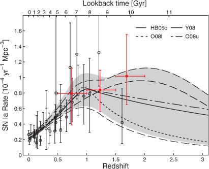
Happily, it appears that the picture is finally clarifying and converging with respect to the field SN Ia rate as a function of redshift, and the DTD that it implies. Rodney & Tonry (2010) have presented a re-analysis of the data of Barris & Tonry (2006), with new SN Ia rates that are lowered, and in much better agreement with other measurements at similar redshifts. Accurate new rates from the Supernova Legacy Survey (SNLS; González-Gaitán et al. 2011; Perrett et al., in preparation; see also Kistler et al. 2011) agree with the revised numbers, and suggest an SN Ia rate that continues to rise out to z = 1, albeit growing more gradually than the SFH. Finally, a quadrupling of the initial Subaru Deep Field high-z SN sample, first presented by Poznanski et al. (2007), is resolving the puzzle of the SN rate out to z = 2. Graur et al. (2011) present a sample of 150 SNe discovered by ‘staring’ at this single field at four independent epochs, with 2 full nights of integration per epoch. SN host galaxy redshifts are based on spectral and photometric redshifts, from the extensive UV to IR database existing for this field. Classification of the SN candidates is photometric. The SN sample includes 26 events that are fully consistent with being normal SNe Ia in the redshift range 1.0 < z < 1.5, and 10–12 such events at 1.5 < z < 2.0. The rates derived from the Subaru data, now based on much better statistics than the GOODS results, merge smoothly with the most recent and most accurate rate measurements at z < 1, confirming the trend of an SN Ia rate that gradually levels off at high z, but does not dive down, as previously claimed by Dahlen et al. (2004, 2008). Graur et al. (2011) find that a DTD with a power-law form,  , when convolved with a wide range of plausible SFHs, gives an excellent fit to the observed SN rates. Their formal result for the power-law index is
  (random error, due to the uncertainties in the SN rates), ±0.17 (systematic error, due to the range of possible SFHs). This conclusion is further confirmed when the Perrett et al. SNLS rates are also included in the fits (Kistler et al. 2011). The field-survey volumetric SN rates and fits are shown in Figure 2. In addition to the works already mentioned, this includes SN rates from Cappellaro et al. (1999), Hardin et al. (2000), Pain et al. (2002), Madgwick et al. (2003), Tonry et al. (2003), Blanc et al. (2004), Neill et al. (2006, 2007), Botticella et al. (2008), Dilday et al. (2008, 2010a), Horesh et al. (2008), and Li et al. (2011b). Additional high-z rates have been recently presented by Barbary et al. (2011), and are consistent with this picture.
|
 . The shaded area is the combined 68% confidence region resulting from the statistical uncertainties in the rates, and the different possible SFHs.
3.2.3 SN Ia Rate versus Galaxy ‘Age’
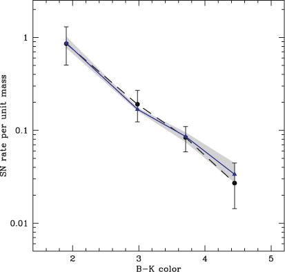
Another approach to recovering the DTD has been to compare the SN rates in galaxy populations of different characteristic ages. It is this approach that gave the first clear indications for a range of delay times in the DTD. Mannucci et al. (2005, 2006), analyzing the Cappellaro et al. (1999) SN sample, discovered that the SN Ia rate per unit stellar mass depends on host galaxy parameters that trace the star-formation rate, such as Hubble type or color. On the other hand, early-type galaxies with no current star formation still have a non-zero SN Ia rate. This observation is shown in Figure 3. The dependence of SN rate on host color was confirmed by Sullivan et al. (2006) for the SNLS sample as well. Both groups interpreted this result to indicate the co-existence of two SN Ia populations, a ‘prompt’ population that explodes within ~100–500 Myr, and a delayed channel that produces SNe Ia on timescales of order 5 Gyr. This led to the ‘A+B’ formulation (Mannucci et al. 2005; Scannapieco & Bildsten 2005), in which the SN Ia rate in a galaxy is proportional to both the star-formation rate in the galaxy (through the B parameter, or through the core-collapse SN rate in Mannucci et al. 2005) and to the stellar mass of the galaxy (through the A parameter).
|
 . Here the mass is the existing stellar mass at the time of observation, assuming the
  DTD. In the model, each galaxy color corresponds to an exponential SFH with some characteristic timescale, such that the observed present-day color is reproduced. Each SFH, when convolved with a t–1.1 DTD, reproduces the observed rates. The shaded area is the uncertainty in the predictions due to the uncertainty in the galaxy stellar populations (see
 In essence, however, A+B is just a DTD with two coarse time bins. The B parameter, divided by the assumed duration of the prompt component, is the mean SN rate in the first, prompt, time bin of the DTD. The A parameter (after correcting for stellar mass loss, m(t), of an old population, always about a factor of 2), is the mean rate in the second, delayed, time bin. In retrospect, these two ‘channels’ appear to be just integrals over a continuous DTD on two sides of some time border (Greggio et al. 2008). And the prompt and delayed SN Ia rates corresponding to A and B define the logarithmic slope and normalization of a power law. Because of the broad range of the time interval over which the DTD is effectively averaged to yield the A parameter, this parameter is really just a rough approximation to the mean of the DTD in this range, a mean that will vary among populations with diverse SFHs. Nevertheless, a t–1 power law is roughly consistent with the measured values of A and B, as seen in Figure 4, where A and B are the medians of the values compiled by Maoz (2008).
|
The directly observed dependence of the SN Ia rates on host galaxy color, as seen in Figure 3, can be very well reproduced by a model that assumes a ~t–1 DTD (the same was shown by Greggio 2005, for some of her DD models). In the model results shown here, each galaxy color corresponds to an exponential SFH with some characteristic timescale, such that the observed present-day color is reproduced. Each SFH, when convolved with a t–1.1 DTD, reproduces the observed rates (see Mannucci et al. 2006 for details).
Totani et al. (2008) used a similar approach to recover the DTD, by comparing SN Ia rates in early-type galaxies of different characteristic ages, seen at z = 0.4–1.2 as part of the Subaru/XMM-Newton Deep Survey (SXDS) project. They were the first to show observationally that the DTD is consistent with a t–1 form. The Totani DTD is also shown is Figure 4.
Additional recent attempts to address the issue with the ‘rate versus age’ approach have been made by Aubourg et al. (2008), Raskin et al. (2009), Yasuda & Fukugita (2009), Cooper et al. (2009), Schawinski (2009), and Thomson & Chary (2011). They have generally confirmed the existence of ‘prompt’ SNe Ia, although with quite a wide range in defining the age of that population. Furthermore, some of these studies have compared, a posteriori, the properties of galaxies that were seen to host SNe, to the properties of matched ‘control samples’ of other galaxies. The risks of such a procedure are discussed in Section 7.
While the concept of a typical age for a host galaxy, interpreted as an SN Ia progenitor age (e.g. Totani et al. 2008), has been useful, it is nonetheless only a rough (and often risky) zeroth-order approximation to the full SFH of a galaxy. The average SN Ia rate from a stellar population is not the same as the SN Ia rate of the average stellar population. Mannucci (2009) has shown some concrete examples of how galaxies with similar mean ages, but with different age distributions, can have SN rates that differ by orders of magnitude. For example, as little as 0.3%, by mass, of young (108 yr) stars that are added to an old (1010 yr) galaxy can easily boost its SN Ia rate by a factor of two. The galaxy remains old-looking, the mass-weighted mean age does not change much, but the observed rate is not due to the DTD at that delay. A DTD recovery method that avoids this approximation is described next.
3.2.4 SN Ia Rate versus Individual Galaxy Star-Formation Histories
Both of the approaches described above, rate versus redshift and rate versus age, involve averaging, and hence some loss of information. In the first approach, one averages over large galaxy populations, by associating all of the SNe detected at a given redshift with all of the galaxies of a particular type at that redshift.In the second approach, as already noted above, a characteristic age for a sample of galaxies replaces the detailed SFH of the individual galaxies in an SN survey. Maoz et al. (2011) presented a method for recovering the DTD which avoids this averaging. In the method, the SFH of every individual galaxy, or even every galaxy subunit, is convolved with a trial universal DTD, and the resulting current SN Ia rate is compared to the number of SNe the galaxy hosted in the survey (generally none, sometimes one, rarely more). DTD recovery is treated as a discretized linear inverse problem, which is solved statistically. Since the observed numbers of SNe are always very small, Cash (1979) statistics are used. Maoz et al. (2011) applied the method to a subsample of the LOSS galaxies, and the SNe that they hosted (Leaman et al. 2011; Li et al. 2011a,b). From the 15 000 LOSS survey galaxies, they chose subsamples having spectral-synthesis-based SFH reconstructions by Tojeiro et al. (2009), based on spectra from the SDSS. In the recovered DTD (Figure 5), Maoz et al. (2011) find a significant detection of both a prompt SN Ia component, that explodes within 420 Myr of star formation, and a delayed SN Ia with population that explodes after >2.4 Gyr.

|
A closely related DTD reconstruction method has been applied by Brandt et al. (2010) to a different sample, the SNe Ia from the SDSS II survey (Frieman et al. 2008; Sako et al. 2008), conducted by repeatedly imaging Stripe 82 of the SDSS. Brandt et al. (2010) also used Tojeiro et al. (2009) SFHs, with the same time bins. However, rather than directly fitting the actual number of SNe observed per galaxy, as done by Maoz et al. (2011), they aimed to reproduce the mean spectrum of the SN host galaxies. Like Maoz et al. (2011), they detected both a prompt and a delayed SN Ia population. We have applied the Maoz et al. (2011) algorithm also to an SDSS-II sample that is similar to the Brandt et al. (2010) sample, but is selected somehwat differently and is larger (Maoz & Mannucci, in preparation). With this larger sample we detect, at 4 σ significance, not only the prompt and delayed components of the DTD, but now also the intermediate, 0.42 < τ < 2.4 Gyr, component of the SN Ia DTD. Figure 5 shows together our SDSS-I and SDSS-II DTD reconstructions, and their good agreement with a t–1 power law.
Brandt et al. (2010) used the ‘stretch parameter’, s, of the SN light curves, to divide their SN Ia sample into a ‘high-stretch’ subsample and a ‘low-stretch’ one, and derived the DTD for each subsample. They found that luminous, high-stretch, SNe Ia tend to have most of their DTD power at short delays, while low-stretch, underluminous, SNe Ia have a DTD that peaks in the longest-delay bin. This is the first derivation of a bivariate DTD,  , albeit with just three delay-time bins and two stretch bins. (Here, DTD is no longer an appropriate name, as this is now the bivariate distribution of delay times and stretches. A more suitable name, as in other fields, would be the bivariate response, or transfer, function, e.g. Bentz et al. 2010). The bivariate SN Ia response function is the thing to aim for in future surveys, that will have large numbers of well-characterized SNe, found among samples of galaxies with well-modeled SFHs. The bivariate response contains information that is additional to the distribution's univariate projection, the DTD, as it gives not only the age of the progenitor systems but also the run of explosion energies for each progenitor age.
3.2.5 SN Remnants in Nearby Galaxies with SFHs Based on Resolved Stellar Populations
Another application of the idea to reconstruct the DTD while taking into account SFHs, rather than mean ages, was made by Maoz & Badenes (2010). They applied this method to a sample of 77 SN remnants in the Magellanic Clouds, which were compiled in Badenes, Maoz, & Draine (2010). The Clouds have very detailed SFHs in many small individual spatial cells, obtained by Zaritsky & Harris (2004) and Harris & Zaritsky (2009), by fitting model stellar isochrones to the resolved stellar populations. Thus, one can compare the SFH of each individual cell to the number of SNe it hosted (or did not) over the past few kyr, as evidenced by the observed remnants. This turns the remnants in the Clouds into an effective SN survey, although several complications need to be dealt with (see Badenes et al. 2010 and Maoz & Badenes 2010). The SFHs are much more detailed and reliable than those based on stellar population synthesis of integrated galaxy spectra. As there is no way to distinguish between core-collapse and Ia SNe in old remnants, a very early DTD bin, at delays 0 < τ < 35 Myr, is included in the reconstruction; the signal in that bin is due to the core-collapse SNe. Unfortunately, since the time-integrated ratio of core-collapse SNe to SNe Ia from a stellar population is about 5:1 (Maoz et al. 2011), only about a dozen of the Cloud remnants are from SNe Ia. This small number of remnants, with the attendant large statistical errors, means that the SN Ia part of the DTD (at τ > 35 Myr) can be binned, at most, into two time bins. Nevertheless, Maoz & Badenes (2010) find a significant detection of a prompt (this time 35 < τ < 330 Myr) SN Ia component. An upper limit on the DTD level at longer delays is consistent with the long-delay DTD levels measured with other methods. The ratio between the rates of prompt and delayed SNe Ia is again consistent with expectations from t–1. This is shown in Figure 6. Larger samples can be produced in the future via ongoing and proposed deep radio surveys for the SN remnant populations in additional nearby galaxies, such as M33 and M31, and by using their spatially differentiated SFHs, again based on the resolved stellar populations.
|
An objection that may arise when considering this approach is that one cannot correctly deduce SN delay times by comparing, on the one hand, star formation rates in a small projected piece of a galaxy to, on the other hand, the SNe that this region of the galaxy is seen to host, since random velocities cause the SN progenitor, by the time it explodes, to have drifted far from its birth location. While this objection is indeed valid if one is comparing SN numbers to the mean stellar ages at their locations, it does not apply if, as here, we are considering detailed SFHs (rather than mean ages), for full ensembles of galaxy cells and SNe. The reason is that both the SN progenitors and their entire parent populations undergo the same spatial diffusion within a galaxy over time. This is explained in more detail, and with some examples, in Maoz et al. (2011) and Maoz & Badenes (2010).
4 Synthesis
4.1 The Form of the DTD
To synthesize the results reviewed above, Figure 7 shows, on one plot, the DTD measurements described previously: the DTD based on galaxy-cluster SN Ia rates (Maoz et al. 2010); the DTD from the ages of high-z field ellipticals (Totani et al. 2008); the DTD from the nearby LOSS galaxies with their SDSS-based SFHs, and the SNe they hosted (Maoz et al. 2011); the DTD from all SDSS-II galaxies having spectroscopic SFH reconstructions, and their SNe (Maoz & Mannucci, in preparation); the DTD from the Magellanic Cloud SN remnants by Maoz & Badenes (2010); and (solid curve) a t–1 power-law DTD that provided a good fit the volumetric field SN rates, when compared to the cosmic SFH (Graur et al. 2011, see Figure 2). Except for this last DTD, all measurements are at the levels that emerge from the data themselves — there has been no vertical adjustment of the points to each other. Figure 8 shows the same data, but on a logarithmic time axis that illustrates more clearly the situation at short time delays.
|
The picture emerging from Figure 7 and 8 is remarkable. For one, all of these diverse DTD determinations, based on different methods, using SNe Ia in different environments and at different redshifts, agree with each other, both in form and in absolute level. At delays t > 1 Gyr, there seems to be little doubt that the DTD is well described by a power law of the form t–s, with s ≈ 1. At delays t < 1 Gyr, the picture is perhaps not as clear-cut. Nonetheless, it is clear that the DTD does peak in that earliest time bin. It may continue to rise to short delays with the same slope seen at long delays, or it may transit to a shallower or steeper rise, but it certainly does not fall. The explosion of at least ~1/2 of SNe Ia within 1 Gyr of star formation is, by now, probably an inescapable fact. The solid curve plotted in Figures 7 and 8 is
Its integral over time between 40 Myr and 10 Gyr is  10–3 M⊙–1.
Recalling the generic predictions of theoretical models, described in Section 3.1, the observed DTD is strikingly similar to the simplest expectations from the DD model, namely an approximately t–1 power law extending out to a Hubble time. The SD models, we recall, though having a rich variety, tend to predict no SNe Ia at delays greater than a few Gyr (with the exception of models that succeed in producing an efficient red-giant donor channel). At face value, the observed results would mean that SD SNe Ia do not play a role in producing the DTD tail clearly seen at long delays in the observations. However, the present data cannot exclude also an SD contribution at short delays, present in tandem with a DD component that produces the ~t–1 power law DTD at long delays.
4.2 The Normalization of the DTD
Apart from the form of the DTD, there is also fairly good agreement (though perhaps some tension), among all the derivations on the DTD normalization, or equivalently its integral between 40 Myr and a Hubble time,  , that is, the time-integrated number of SNe Ia per stellar mass formed. Table 1 summarizes these numbers (as always, with a consistent assumed IMF — the Bell et al. 2003 diet Salpeter IMF that simulates a realistic IMF with a low-mass turnover).
|
Several of the normalizations appear nicely consistent with  , in units of 10–3 M⊙–1. One exception to this, on the high side, is the number based on the iron mass content of galaxy clusters,
  . This number, which is based on cluster iron abundance, gas fraction, and assumed core-collapse SN iron yield, sets the lowest-delay bin in the DTD from clusters. However, as seen in Figures 7 and 8, the other cluster DTD points, which come directly from cluster SN rate measurements (rather than from the iron constraint), appear to be in good agreement with most of the DTDs from other methods. This is also seen quantitatively in Table 1, which gives the best-fit
  normalizations, and 1σ errors, based on the cluster SN rates alone, assuming a DTD of the form t–1, or t–0.9 (the cluster rates alone do not well constrain the power-law index). This suggests that there may be an error in one or more of the assumptions of the iron-based point: the iron abundance, or the gas to stellar mass ratio in clusters may have been systematically overestimated; or the contribution of core-collapse SNe to cluster iron enrichment may be underestimated, for example, if pair-instability SNe are major iron suppliers (e.g., Quimby et al. 2011; Kasen et al. 2011). It has been pointed out (Bregman et al. 2010) that the roughly constant iron abundance in galaxy clusters of different total masses, despite the large range in their gas to stellar mass ratios, indicates a major source of iron that is unrelated to the present-day stellar population in cluster galaxies. Similar conclusions have been reached from the analysis of radial abundance gradients in clusters (Million et al. 2011).
Another high  value comes from the SN remnants in the Magellanic Clouds. Here, it is quite possible that the short-delay bin is contaminated by core-collapse SNe, and hence is overestimated (see Maoz & Badenes 2010). Furthermore, the overall normalization in this case rests on the assumption that all stars above 8M⊙ produce core-collapse SNe, an assumption that may not hold if some fraction of such stars collapse directly into black holes (e.g., Horiuchi & Beacom 2011), in which case
  would be reduced correspondingly.
Deviating on the low side, the volumetric field SN Ia rates versus redshift suggest  . This could be an indication that most SFH estimates have been overestimated, perhaps due to over-correction for extinction, by 50%, or even a factor of 2 (see discussion of this point in Graur et al. 2011). It is hard to believe that the lower
  value implied by the volumetric rates is a real effect, due to environment, metallicity or evolution, for example, since some of the measurements (e.g., galaxy clusters) that give high
  values span redshift ranges that are similar to those of the volumetric measurement, and others (e.g. SDSS-II) were obtained in environments that are similar to those of the volumetric one. It thus remains to be seen whether the current observed range of
  will turn out to indicate a real spread; or to be the result of a universal value that is somewhere in this range, perhaps
  , but that is affected in some cases by random and systematic errors.
Compared to these observed DTD normalizations, the theoretical DD models do not fare too well. As already noted by Maoz (2008), Ruiter et al. (2008), Mennekens et al. (2010), and Maoz et al. (2010), binary synthesis DD models underpredict observed SN rates by factors of at least a few, and likely by more. One way of alleviating this inconsistency with the observations would be to include sub-Chandra mergers in the accounting (see Section 5, below). Alternatively, Thompson (2010) has proposed that at least some of the SN Ia progenitors may be triple systems, consisting of a WD–WD inner binary and a tertiary that induces Kozai (1962) oscillations in the inner binary, driving it to higher eccentricity and shortening the time until a gravitational wave–driven merger between the two WDs. The possibility of detecting such triple systems through their gravitational-wave signals is explored by Gould (2011). Another rate-enhancement scenario is through an increase in the number of close binaries, if most SNe Ia occur in star clusters. Dynamical encounters between binaries and other cluster stars will harden the binaries (Shara & Hurley 2002). The effect has been used to explain the enhancement in the number of low-mass X-ray binaries observed in globular clusters (Sarazin et al. 2003). However, Washabaugh & Bregman (2011) place upper limits on the presence of globular clusters at the locations of SNe Ia in elliptical galaxies observed with HST, thus ruling out globular clusters as a significant global SN Ia rate enhancement mechanism.
5 So, Where are Those Pre-Merger WD Binaries?
If DD mergers produce SNe Ia, the progenitor systems should be around us. It is actually easy to estimate quite accurately what fraction of local WDs must be SN Ia progenitors, in order to explain the SN Ia rate in the context of the DD scenario. From the LOSS survey, the SN Ia rate per unit stellar mass in large-ish SBc galaxies is about 1× 10–13 yr1 M⊙–1 (Li et al. 2011b). We live in a typical region (the disk) of such a galaxy. In the solar neighborhood the ratio of stellar mass to WD number is 18.5 M⊙/WD (based on the local stellar mass density, 0.085 M⊙pc–3, McMillan 2011; and the local WD number density, 0.0046 pc –3, Harris et al. 2006). Multiplying the SN Ia rate by the stellar mass to WD ratio, and by a Hubble time, 2.5% of local WDs should be SN Ia progenitors that will merge within a Hubble time. (This assumes a roughly constant star-formation rate in the disk, which would lead to a constant, steady-state, SN rate.) We note that this estimate circumvents the large uncertainties in the total stellar mass of the Galaxy, its SN rate, and its SFH, uncertainties which normally enter such estimates.
As already noted, SPY (Napiwotzki et al. 2004; Geier et al. 2007) surveyed ~1000 local WDs and found no binaries that will clearly end up as super-Chandra mergers within a Hubble time. According to the above estimate, there should have been about 25 such systems, if the super-Chandra DD scenario is to explain the SN Ia rate. The efficiency of SPY has not been reported, but it is unlikely to be so low, and hence this null result argues against this scenario. On the other hand, one must remember that all observed WD samples are flux limited. This might select samples of WDs with binarity fractions and mass distributions that are distinct from those of the true DD progenitor population, which might remain unobserved.
The ongoing SWARMS survey by Badenes et al. (2009) is searching for close binaries among the WDs observed in the SDSS spectral survey. All SDSS spectra were originally split into sub-exposures for the purpose of cosmic-ray rejection. Some sub-exposures are separated by ~ 15 min, sometimes by much more, and this permits searching for radial-velocity variations due to the orbital motions of close DD binaries. Although the SDSS spectra have much lower spectral resolution than SPY (70 km s–1 and 16 km s–1, respectively), SDSS is a larger sample, and each WD has, on average, more epochs (increasing the chances to ‘catch’ a change in radial velocity).
Badenes & Maoz (in preparation) take a statistical approach to address this question in the SWARMS database. Rather than finding all the binaries and characterizing their orbits, they find, for each WD in SWARMS, the maximal radial-velocity difference among all its epochs. They then derive the observed distribution of those maximum velocity differences. The distribution probes the parameters of the local WD binary population — binarity fraction, initial separation distribution, and mass ratio distribution. To constrain those parameters, Badenes & Maoz produce a grid of simulated present-day binary populations. These binaries are then ‘observed’ with the same sampling patterns and velocity error distributions as the real data, and the simulated maximum velocity difference distribution is derived for each model. The region of binary-parameter space that gives velocity-difference distributions consistent with the observed one can thus be found. Furthermore, for every model binary population, the WD merger rate can be calculated (whether super-Chandra or in general).
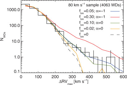
Figure 9 shows the observed SWARMS maximal radial velocity difference distribution, for a sample of 4063 DA-type WDs having velocity errors of <80 km s–1 per epoch. The smooth curves show four different WD binary population models, two that reproduce the data well, and two that are rejected. The observations thus have the power to discriminate among models.
|
Intriguingly, the binary population models that do reproduce the observed velocity-difference distribution have a super-Chandra WD merger rate that is an order of magnitude too low to account for the SN Ia rate, as speculated above based on the SPY null result. However, the general WD merger rate (i.e., all merged masses), is remarkably similar to the SN Ia rate requisite, 1× 10–13 yr–1 M⊙–1. For some plausible assumptions about the primary and secondary mass distributions of the WDs, the majority of those mergers will be similar-mass mergers (e.g., 70% will have mass differences less than 0.2 M⊙, and 40% less than 0.1 M⊙) and with total masses not too far below the Chandrasekhar mass. This raises again the scenario of sub-Chandra DD mergers as a way of explaining all SNe Ia (e.g. van Kerkwijk et al. 2010; Guillochon et al. 2010; Ruiters et al. 2011). Apart from the the increased numbers, sub-Chandra merger products have lower central densities. Detonations at such densities may give SN ejecta with the correct mix of iron-peak elements, intermediate-mass elements, and unburned carbon and oxygen, without resorting to the deflagration-delayed detonation scheme.
6 Additional SN Ia Rate Phenomenology, Explained or Not
In the course of the SN Ia rate studies of the past few years, various dependences of SN Ia rates on host galaxy properties and environments have been seen. We briefly review them here, comment on their current observational status, and on whether they are naturally explained in the context of the recent developments concerning the DTD.
6.1 Enhanced SN Rates in Radio Galaxies
Della Valle & Panagia (2005) and Della Valle et al. (2005), analyzing the Cappellaro et al. (1999) SN sample, found a factor-of-4 enhancement of the SN Ia rate in radio-loud early-type galaxies, compared to radio-quiet ones. They interpreted this as evidence for a population of SNe Ia with an ~100 Myr delay after star formation. The idea was that an episode of gas accretion or capture of a galaxy fuels the central black hole, producing the radio luminosity, while simultaneously triggering star formation. Assuming the lifetime of the radio phase is ~100 Myr, the enhanced SN Ia rate would be associated with progenitors of this age in starburst population. An objection to this interpretation (Greggio et al. 2008) was that the same radio galaxies (always early types) were never seen to host the core-collapse SNe that one would also expect from a young starburst. Some support for the higher SN Ia rates in radio galaxies, though not highly significant, has been found in the SNLS sample by Graham et al. (2010). The issue should be resolved soon by comparison of the radio-loud and radio-quiet rates in the LOSS sample (Li et al. 2011a,b).
6.2 Enhanced SN Rates in Galaxy Clusters
There have also been reports of enhanced SN Ia rates in cluster early-type galaxies, as opposed to field ellipticals. Mannucci et al. (2008) found such an enhancement in the Cappellaro et al. (1999) sample, while noting it was only marginally significant. Recent results by Sand et al. (2011) give a low-z cluster rate that is intermediate to the field and cluster elliptical rates of Mannucci et al. (2008), but consistent with both to within errors. Thus, a cluster rate enhancement is not yet rejected, but its reality is questionable.
6.3 The SN Rate–Size Relation
Most recently, Li et al. (2011b) have discovered a ‘rate–size relation’ in the LOSS data. Among SNe Ia hosted by specific Hubble types of galaxies, the rate per unit mass depends on various measures of host-galaxy ‘size’, such as mass or infrared luminosity. Such an effect is expected in star-forming galaxies, because of the known anticorrelation between galaxy mass and specific star formation (e.g., Schiminovich et al. 2007). However, the effect is seen even in the early-type hosts in LOSS, although its significance in that case is low. Following Mannucci et al. (2005), Li et al. (2011b) estimated galaxy stellar masses using B and K magnitudes. The rate–size relation could be an artifact of the uncertainties involved in this approach, for example, due to the effects of the mass–age, mass–metallicity relations (Tremonti et al. 2004), or the star formation rate–mass–metallicity relations (Mannucci et al. 2011). Nonetheless, Kistler et al. (2011) have shown that the LOSS rate–size relation, even in the early-types, can be reproduced at the observed level, based on a t–1 DTD, and the pheonomenon of ‘downsizing’. More massive galaxies were, on average, formed at earlier epochs (e.g., Gallazzi et al. 2005; Pozzetti et al. 2010; Rettura et al. 2011; Kajisawa et al. 2011). When observing a massive early-type galaxy, which is older than a less-massive one, we are looking further down the tail of the DTD, and therefore measure a lower SN Ia rate.
6.4 The SN Stretch–Host Age Relation
As already noted, the relation between host galaxy ‘age’ and SN Ia luminosity, or stretch, has been known for some time, and even roughly quantified in the framework of the DTD picture (Brandt et al. 2010). It is not hard to imagine, at least in principle, a physical scenario that would lead to such a relation (see, e.g., Greggio 2010). For example, in the DD picture, the post–common envelope WD separation might be a function of the total WD mass, with more massive binaries having smaller initial separations than the low-mass pairs. This would naturally lead to a dependence between delay time and explosion energy. It remains to be seen whether such a trend is realized in practice, in models or in observations of WD binary populations.
7 Sins of SN Rate Measurement, and an Analogy
Measuring and analyzing SN rates is, in principle, straightforward, but there are pitfalls where some have gone astray. We believe it may be useful to list the main ones we have encountered in the literature (without citing the offenders: you know who you are). Most of these are self-explanatory.
7.1 The Seven Deadly Sins
-
Not using proper detection efficiency simulations.
-
Not properly calculating the visibility time of your survey.
-
Using heterogeneous compilations of SNe from surveys with unknown sensitivities to estimate rates.
-
Not stating the assumptions about parameters entering your rate normalization, such as IMF, H0 and formed mass versus existing mass.
-
Comparing rates without accounting for the effects of different assumed normalization parameters in different studies.
-
Ignoring or not presenting the systematic errors in your rates or analysis, such as uncertainties in extinction, SFH, or host population age distribution.
-
Comparing a posteriori the properties of SN host galaxies to those of a different ‘control sample’.
The seventh sin has been often committed in recent years, but it is perhaps the one whose sinfulness requires the most subtlety to understand. What is wrong, after all, with this approach? We observe in detail some specific galaxies that have been seen to host SNe. We compare some properties of the SN hosts to those properties as found in some general sample of galaxies that seems to be matched to the SN host sample in mass, redshift, luminosity, and so on. One would think that any differences we find must then reflect something about the SN progenitors. For example, if we find an excess of stars of a given age in the SN host galaxies, would not this indicate the age of the SN progenitor systems when they explode? Unfortunately, the answer is ‘maybe’, or often ‘no’. The problem is that, even though we have made an effort to choose a ‘good’ control sample, it is still a different sample from the sample that was actually monitored for SNe, and from which the host galaxies are drawn (and often, we do not even know what that monitored sample was, or it might be a heterogeneous compilation of samples with diverse selection criteria). As such, there is a great risk that there are some properties that are different in the SN host sample and in the control sample, but which have nothing to do with the presence of SNe in the host sample. We illustrate this with an analogy.
7.2 The Parable of the Martian Scientists
Imagine that the Martians have been studying Earth and its inhabitants for a while. After the less-than-hospitable reception they received at Roswell in the mid-20th century, they have wisely decided to stick to remote sensing observations. They have developed very high resolution techniques, and are capable of detecting individual humans on Earth. Although they are not yet aware of the phenomena of growth and aging that characterize Earth-bound life, the Martians have noticed that humans have a range of properties (e.g., sizes, speeds) which they quantify with a parameter that we would call ‘age’. (And, in the future, long after the Martian scientists it will have understood the human life cycle, they will continue to refer to elderly people as ‘early-type humans’, and to young people as ‘late-type humans’, just for the sake of confusing their students and themselves!)
One research topic of great interest among the Martian Earthonomers is ‘baby humans’. The Martians have realized that babies must play some important role in human physiology. The Martians have developed sensitive techniques to detect human babies, based on their particular audio-spectral signatures (which we call cries). Even some amateur Martian Earthonomers have become quite adept at discovering babies in this way. The value of baby detections further increased when it was realized by the Martians that human babies have a narrow distribution of sizes at birth, with a dispersion of only 14% (Subramanian et al. 2005). As such, they serve as excellent ‘standard rulers’ for setting the scale in the highest-resolution images, and are thus essential for mapping the Earth. However, the physical nature of those same babies is not yet understood. Indeed, a fierce debate continues among the Martians on the question of who are the progenitors of the babies: Are they other humans, of a certain age? Or are babies perhaps created artificially or spontaneously in some process? Various theoretical progenitor scenarios having been proposed in the Martian scientific literature. Unfortunately, the birth of babies invariably occurs in optically thick structures (which we call hospitals, houses, huts), making a direct resolution of the question impossible.
The amateur Earthonomers have discovered that they can reap a large harvest of baby discoveries if they focus their instruments, which can cover Earth scales of a few hundred km at a time, on particular regions. For example, an amateur monitoring the region that we know as Afghanistan might be able to spot a few thousand new babies in a single night! Some professional Martian Earthonomers decide to exploit this growing database on new babies to address the baby progenitor question. Using pointed observations, they measure the human populations of a sample of individual houses that were reported by the amateurs to have hosted new babies. Many of these houses are in Afghanistan. However, no Martian study exists of the human population in Afghanistan as a whole, nor are the heterogenous selection criteria and the effective monitoring times used by the amateurs known. The professionals therefore compare the properties of the human population in the Afghan baby host houses to a ‘control sample’ for which a population study is already available. Among the few available options, they choose a study that was done in the region that we call Spain. This seems like a reasonable choice. Spain and Afghanistan have comparable areas, geographic latitudes, and population sizes. The Spanish human population study seems all the more suited as it gives populations per house, and many of the Afghan births indeed take place in houses, as opposed to the larger structures (hospitals) where baby births often take place in other regions.
From their comparison of samples, the Martians quickly discover that the human age distribution in the Afghan baby host houses is significantly different from the age distribution in the Spanish control sample. First, there is an excess in the Afghan host houses of humans that are about 20–40 years old, supporting some previous theoretical speculation that this is the age of the baby progenitor human population. However, in the Afghan houses there is an even larger excess of humans aged 1–15, a population that is quite rare in the Spanish control sample. The Martians promptly conclude that there is a bimodal baby progenitor distribution: some babies derive from humans that are 20–40 years old, and some from humans that are 1–15 years old (remember, the Martians are not aware of the process of growth and aging, whereby babies become adolescents and then adults). The Martians, furthermore, note another striking difference. The Afghan baby host houses have a deficit of humans aged 45–80, compared to the Spanish control sample. Perhaps, they speculate, there is a third baby production channel, in which old humans are transformed into new babies?
The problem, of course, is that despite their best intentions, the Martians have been comparing a baby host sample and a control sample that are not well matched. Afghanistan has one of the highest rates of births per capita on Earth, while Spain has one of the lowest. Every baby that is born in Afghanistan is likely to have a good number of siblings living in the same house, and it is they that constitute the age 1–15 excess population that the Martians are seeing. A Spanish baby, in contrast, is most likely to have no siblings. And, sadly, Afghanistan has among the shortest life expectancies in the world, while Spain has among the longest, and this is the true reason for the deficit of older people in the Afghan sample.
Of course, things need not have turned out so incorrectly for the Martians. They might have chosen for their control sample a region with an age distribution that is more similar to that of their host sample. But the only way of being sure that their control sample is in fact adequate would have been to measure the properties of the same population that was monitored for babies, and for the whole of that population (or at least a randomly selected, properly weighted subsample of it). Had they done so, they would have found that the presence of ~20–40 year-old humans is a more or less necessary condition for the appearance of a new baby, be it in a dwelling in Spain or in Afghanistan, while the presence or absence of the other age groups is not. If, furthermore, the Earthonomers could figure out the exact time periods during which each house was monitored for babies that could have been detected (the visibility time), they would be able to reconstruct the birth rate as a function of progenitor age — the baby delay time distribution. With carefully measured samples having enough babies for good statistics, they would be able to gain important insights about human physiology and society. For example, they would see that the DTD is shifted to larger delays in Spain compared to Afghanistan, reflecting the sociological trend in Western societies for a later child-bearing age.
8 Conclusions
In summary, a host of measurements over the past few years have revealed an increasingly clear picture of the SN Ia DTD. It is well described by a power law of index ≈ –1, going out to a Hubble time. At delays of <1 Gyr, this shape may continue, or the slope may change somewhat. The time-integrated SN Ia production efficiency is about 2 ± 1 SN Ia events for every 1000 M⊙ formed in stars, that is, it is now known to better than a factor of 2. (This is often expressed as the fraction of 3–8M⊙ stars that eventually explode as SNe Ia; the above range translates to 3–10%.) The uncertainties regarding the shape and normalization of the DTD are dominated by the uncertainties in the monitored galaxy stellar populations and the SFH.
The observed DTD form is strikingly similar to the form generically expected, due to fundamental gravitational wave physics, in the DD scenario. The efficiency of SN Ia production by detailed models still falls short of the observed number, by at least a factor of a few. The competing SD model makes predictions that differ from the observations both in DTD form and in the absolute numbers of SNe. Given the disagreement among the SD calculations themselves, it is not yet clear whether this is a problem of the SD model or of its calculation. But, keeping all these caveats in mind, the current picture appears to support the DD model. In the process, several of the puzzles that have arisen concerning SN Ia rates, as reviewed above, have been explained or have disappeared. The local WD population appears to have an insufficient number of close binaries that will merge within a Hubble time as super-Chandra objects, according to the classical DD picture. If however, it is sub-Chandra mergers that produce normal SNe Ia, there may, in fact, be enough such binaries to reproduce the SN Ia rate.
In terms of the future, several developments are unfolding. Two ongoing multi-cycle treasury (MCT) programs with HST, CLASH (Postman et al. 2011) and CANDELS (Grogin et al. 2011; Koekemoer et al. 2011) aim to measure the SN rate out to z = 2 and perhaps even somewhat beyond. This can sharpen our view of the shorter delay times in the DTD, and test for the influence of other parameters, such as metallicity, on the rates (e.g., Gallagher et al. 2008; Meng & Yang 2011a; Bravo & Badenes 2011; Kistler et al. 2011). Deep radio surveys for SN remnants with the EVLA will produce large samples of remnants in additional Local Group galaxies, beyond the Magellanic Clouds. Ongoing high-resolution imaging of those same galaxies with HST will produce the data for region-by-region SFHs based on resolved stellar populations. With these two datsets combined, it will be possible to reconstruct the DTD at short delays, where the greatest uncertainty remains observationally, and where an SD contribution may still play a role. Finally, larger samples of SNe and host galaxies, for example from the upcoming Dark Energy Survey2 and the HyperSuprimeCam Survey with Subaru3 will permit addressing the bivariate SN Ia response function — the next dimension beyond the DTD, which will start to make connections between the progenitors and the observed features of the explosions themselves.
Acknowledgments
We thank Gijs Nelemans and the referee, Laura Greggio, for valuable comments. DM acknowledges support by the Israel Science Foundation. FM acknowledges partial financial support of the Italian Space Agency, through contracts ASI-INAF I/016/07/0 and I/009/10/0, and PRIN-INAF 2008. FM also acknowledges support by NASA through a grant from the Space Telescope Science Institute, which is operated by the Association of Universities for Research in Astronomy, Incorporated, under NASA contract NAS5-26555.
References
Aubourg, É., Tojeiro, R., Jimenez, R., Heavens, A., Strauss, M. A. and Spergel, D. N., 2008, A&A, 492, 631Badenes, C., Hughes, J. P., Bravo, E. and Langer, N., 2007, ApJ, 662, 472
| Crossref | GoogleScholarGoogle Scholar | 1:CAS:528:DC%2BD2sXnsV2lsL8%3D&md5=6ef079ba8847ea12d6286290a176db13CAS |
Badenes, C., Mullally, F., Thompson, S. E. and Lupton, R. H., 2009, ApJ, 707, 971
| Crossref | GoogleScholarGoogle Scholar | 1:CAS:528:DC%2BC3cXptlaqug%3D%3D&md5=7630b24542bb7c0cbec13f3e6102d15cCAS |
Badenes, C., Maoz, D. and Draine, B. T., 2010, MNRAS, 407, 1301
| Crossref | GoogleScholarGoogle Scholar |
Barbary, K., et al., 2010, arXiv:1010.5786
Barbary, K., et al., 2011, arXiv:1110.6442
Barris, B. J. and Tonry, J. L., 2006, ApJ, 637, 427
| Crossref | GoogleScholarGoogle Scholar | 1:CAS:528:DC%2BD28XitFWjsb0%3D&md5=8aa257418a562061dd09c22bf0f4b285CAS |
Bell, E. F., McIntosh, D. H., Katz, N. and Weinberg, M. D., 2003, ApJS, 149, 289
| Crossref | GoogleScholarGoogle Scholar |
Bentz, M. C., 2010, ApJ, 720, L46
| Crossref | GoogleScholarGoogle Scholar | 1:CAS:528:DC%2BC3cXhtF2ktrjN&md5=81c42be7577102100d35eb3a7a482bfeCAS |
Bianco, F. B., et al., 2011, arXiv:1106.4008
Blanc, G. and Greggio, L., 2008, NewA, 13, 606
| Crossref | GoogleScholarGoogle Scholar | 1:CAS:528:DC%2BD1cXntVOgt7w%3D&md5=2fd38486921175d43b8a83e37165142fCAS |
Blanc, G., 2004, A&A, 423, 881
| 1:CAS:528:DC%2BD2cXotlelsLk%3D&md5=6d73ac1a0c753ec8ff27153abb9a1e5fCAS |
Blondin, J. M., Borkowski, K. J., Reynolds, S. P. and Foight, D. R., 2010, Bulletin of the American Astronomical Society, 41, #427.01
Bloom, J. S., et al., 2011, arXiv:1111.0966
Bogomazov, A. I. and Tutukov, A. V., 2009, ARep, 53, 214
| Crossref | GoogleScholarGoogle Scholar | 1:CAS:528:DC%2BD1MXjt1Cju74%3D&md5=c0a1c698f9b0aeebfd8339b038de419bCAS |
Bogomazov, A. I. and Tutukov, A. V., 2011, ARep, 55, 497
| Crossref | GoogleScholarGoogle Scholar | 1:CAS:528:DC%2BC3MXntVekur8%3D&md5=fd7c8c77d707705bd20b4ae164b4c3c0CAS |
Botticella, M. T., 2008, A&A, 479, 49
| 1:CAS:528:DC%2BD1cXktlKrsro%3D&md5=5330c1598d8b0a24366b372ecc6bd5cbCAS |
Brandt, T. D., Tojeiro, R., Aubourg, É., Heavens, A., Jimenez, R. and Strauss, M. A., 2010, AJ, 140, 804
Bravo, E. and Badenes, C., 2011, MNRAS, 414, 1592
| Crossref | GoogleScholarGoogle Scholar | 1:CAS:528:DC%2BC3MXpt1yrtrw%3D&md5=46c8ac820fe59bbb741efa197960bd0bCAS |
Bregman, J. N., Anderson, M. E. and Dai, X., 2010, ApJ, 716, L63
| Crossref | GoogleScholarGoogle Scholar | 1:CAS:528:DC%2BC3cXovV2ksLY%3D&md5=769328d0c8ad41433737da5557f7ac8bCAS |
Brown, P. J., et al., 2011, arXiv:1110.2538
Cappellaro, E., Evans, R. and Turatto, M., 1999, A&A, 351, 459
Cash, W., 1979, ApJ, 228, 939
| Crossref | GoogleScholarGoogle Scholar |
Cassisi, S., Iben, I., and Tornambe, A., 1998, ApJ, 496, 376
| Crossref | GoogleScholarGoogle Scholar | 1:CAS:528:DyaK1cXisFeqtLc%3D&md5=e650bfc62ddb1df92c720f0c1c4a2deaCAS |
Chen, X., Han, Z. and Tout, C. A., 2011, ApJ, 735, L31
| Crossref | GoogleScholarGoogle Scholar |
Chomiuk, L. and Soderberg, A., 2011, ATel, 3597, 1
Chomiuk, L., Soderberg, A. M., Chevalier, R., Badenes, C. and Fransson, C., 2011, Bulletin of the American Astronomical Society, 43, #304.05
Ciotti, L., D'Ercole, A., Pellegrini, S. and Renzini, A., 1991, ApJ, 376, 380
| Crossref | GoogleScholarGoogle Scholar | 1:CAS:528:DyaK3MXlvFeisb0%3D&md5=1a14001e5a61f89887d40578307617b9CAS |
Colbert, J. W., Mulchaey, J. S. and Zabludoff, A. I., 2001, AJ, 121, 808
Cooper, M. C., Newman, J. A. and Yan, R., 2009, ApJ, 704, 687
| Crossref | GoogleScholarGoogle Scholar | 1:CAS:528:DC%2BD1MXhtl2ksrbF&md5=754278b3d564d939619001660eb8e94fCAS |
Cresci, G., Mannucci, F., Della Valle, M. and Maiolino, R., 2007, A&A, 462, 927
| 1:CAS:528:DC%2BD2sXis1ygtrw%3D&md5=e97a74463fc4eb1ebb1dc1e605aa3e57CAS |
Daddi, E., Cimatti, A. and Renzini, A., 2000, A&A, 362, L45
Dahlen, T., 2004, ApJ, 613, 189
| Crossref | GoogleScholarGoogle Scholar | 1:CAS:528:DC%2BD2cXpsVWrsbk%3D&md5=ca2f256341681319c89c4958626941fdCAS |
Dahlen, T., Strolger, L.-G. and Riess, A. G., 2008, ApJ, 681, 462
| Crossref | GoogleScholarGoogle Scholar | 1:CAS:528:DC%2BD1cXptFegtLg%3D&md5=cad1454632dbd9f0705d79fdd63c3bebCAS |
Darbha, S., Metzger, B. D., Quataert, E., Kasen, D., Nugent, P. and Thomas, R., 2010, MNRAS, 409, 846
| Crossref | GoogleScholarGoogle Scholar | 1:CAS:528:DC%2BC3MXmtVyi&md5=f620b794045432293ef86ab235009a37CAS |
Della Valle, M. and Panagia, N., 2003, ApJ, 587, L71
| Crossref | GoogleScholarGoogle Scholar |
Della Valle, M., Panagia, N., Padovani, P., Cappellaro, E., Mannucci, F. and Turatto, M., 2005, ApJ, 629, 750
| Crossref | GoogleScholarGoogle Scholar |
Di Paola, A., Larionov, V., Arkharov, A., Bernardi, F., Caratti o Garatti, A., Dolci, M., Di Carlo, E. and Valentini, G, 2002, A&A, 393, L21
Di Stefano, R., 2010, ApJ, 712, 728
| Crossref | GoogleScholarGoogle Scholar | 1:CAS:528:DC%2BC3cXkvVOlsL4%3D&md5=b53634b31059f7fa02cda41e6c1950cdCAS |
Di Stefano, R., Voss, R. & Claeys, J. S. W., 2011, arXiv:1102.4342
Dilday,, B., 2008, ApJ, 682, 262
| Crossref | GoogleScholarGoogle Scholar |
Dilday,, B., 2010a, ApJ, 713, 1026
| Crossref | GoogleScholarGoogle Scholar |
Dilday, B., 2010b, ApJ, 715, 1021
| Crossref | GoogleScholarGoogle Scholar |
Eisenhardt, P. R. M., 2008, ApJ, 684, 905
| Crossref | GoogleScholarGoogle Scholar |
Foley, R. J., et al., 2011, arXiv:1109.0987
Förster, F. and Schawinski, K., 2008, MNRAS, 388, L74
Förster, F., Wolf, C., Podsiadlowski, P. and Han, Z., 2006, MNRAS, 368, 1893
| Crossref | GoogleScholarGoogle Scholar |
Fuhrmann, K., 2005, MNRAS, 359, L35
Gal-Yam, A. and Maoz, D., 2004, MNRAS, 347, 942
| Crossref | GoogleScholarGoogle Scholar | 1:CAS:528:DC%2BD2cXhsVGis78%3D&md5=5a0b8d9d9e97289e049f88030c95d3efCAS |
Gal-Yam, A., Maoz, D. and Sharon, K., 2002, MNRAS, 332, 37
| Crossref | GoogleScholarGoogle Scholar |
Gal-Yam, A., Maoz, D., Guhathakurta, P. and Filippenko, A. V., 2008, ApJ, 680, 550
| Crossref | GoogleScholarGoogle Scholar | 1:CAS:528:DC%2BD1cXotlWksLw%3D&md5=3f4945ff7cab4d859e909ec76f117da0CAS |
Gallagher, J. S., Garnavich, P. M., Caldwell, N., Kirshner, R. P., Jha, S. W., Li, W., Ganeshalingam, M. and Filippenko, A. V., 2008, ApJ, 685, 752
| Crossref | GoogleScholarGoogle Scholar | 1:CAS:528:DC%2BD1cXht1KqtbnL&md5=b33dc5cdc2dff89d968cccf09df70b95CAS |
Gallazzi, A., Charlot, S., Brinchmann, J., White, S. D. M. and Tremonti, C. A., 2005, MNRAS, 362, 41
| Crossref | GoogleScholarGoogle Scholar | 1:CAS:528:DC%2BD2MXhtVykt7rJ&md5=ba430fe3701851479cae084ab4e04f09CAS |
Ganeshalingam, M., Li, W. and Filippenko, A. V., 2011, MNRAS, 416, 2607
Geier, S., Nesslinger, S., Heber, U., Przybilla, N., Napiwotzki, R. and Kudritzki, R.-P., 2007, A&A, 464, 299
| 1:CAS:528:DC%2BD2sXkvVKrtLs%3D&md5=ff53a1d211b039152d8458510efe66e1CAS |
Geier, S., Heber, U., Kupfer, T. and Napiwotzki, R., 2010, A&A, 515, A37
Gilfanov, M. and Bogdán, Á., 2010, Natur, 463, 924
| Crossref | GoogleScholarGoogle Scholar | 1:CAS:528:DC%2BC3cXitFelsr4%3D&md5=89b51aecbe64aa09c14058db22a688c5CAS |
González-Gaitán, S., 2011, ApJ, 727, 107
| Crossref | GoogleScholarGoogle Scholar |
González Hernández, J. I., Ruiz-Lapuente, P., Filippenko, A. V., Foley, R. J., Gal-Yam, A. and Simon, J. D., 2009, ApJ, 691, 1
| Crossref | GoogleScholarGoogle Scholar |
Gould, A., 2011, ApJ, 729, L23
| Crossref | GoogleScholarGoogle Scholar |
Graham, M. L., 2008, AJ, 135, 1343
Graham, M. L., 2010, AJ, 139, 594
Graur, O., et al., 2011, MNRAS, in press, arXiv:1102.0005
Greggio, L., 2005, A&A, 441, 1055
Greggio, L., 2010, MNRAS, 406, 22
| Crossref | GoogleScholarGoogle Scholar | 1:CAS:528:DC%2BC3cXhtVGit7%2FP&md5=85ebedcbbe0fdc98afaa7b6eb58ee80eCAS |
Greggio, L. and Renzini, A., 1983, A&A, 118, 217
| 1:CAS:528:DyaL3sXhsFWjtr0%3D&md5=c1c38410003218d76ab93d141764685dCAS |
Grogin, N. A., 2011, ApJS, 197, 35
Greggio, L., Renzini, A. and Daddi, E., 2008, MNRAS, 388, 829
| Crossref | GoogleScholarGoogle Scholar |
Guerrero, J., García-Berro, E. and Isern, J., 2004, A&A, 413, 257
Guillochon, J., Dan, M., Ramirez-Ruiz, E. and Rosswog, S., 2010, ApJ, 709, L64
| Crossref | GoogleScholarGoogle Scholar | 1:CAS:528:DC%2BC3cXhvVygur0%3D&md5=bad62b52eed0edd37e5aed314254b85dCAS |
Hachisu, I., Kato, M. and Nomoto, K., 1999, ApJ, 522, 487
| Crossref | GoogleScholarGoogle Scholar |
Hachisu, I., Kato, M. and Nomoto, K., 2008a, ApJ, 679, 1390
| Crossref | GoogleScholarGoogle Scholar | 1:CAS:528:DC%2BD1cXotVahtLY%3D&md5=ea0ce511d62eb232b91d2de35fbc1764CAS |
Hachisu, I., Kato, M. and Nomoto, K., 2008b, ApJ, 683, L127
| Crossref | GoogleScholarGoogle Scholar |
Hachisu, I., Kato, M. and Nomoto, K., 2010, ApJ, 724, L212
| Crossref | GoogleScholarGoogle Scholar |
Hakobyan, A. A., et al., 2011, arXiv:1104.0300
Han, Z. and Podsiadlowski, P., 2004, MNRAS, 350, 1301
| Crossref | GoogleScholarGoogle Scholar | 1:CAS:528:DC%2BD2cXls1Sju7c%3D&md5=5ba70e727757356c3284663fc1d43873CAS |
Han, Z., Podsiadlowski, P. and Eggleton, P. P., 1995, MNRAS, 272, 800
Hancock, P. P., Gaensler, B. M. and Murphy, T., 2011, ApJ, 735, L35
| Crossref | GoogleScholarGoogle Scholar |
Hardin,, D., 2000, A&A, 362, 419
Harris, J. and Zaritsky, D., 2009, AJ, 138, 1243
Harris, H. C., 2006, AJ, 131, 571
| 1:CAS:528:DC%2BD28Xht1yqs7w%3D&md5=15b1e015c71573009916b01a7aeb3a0dCAS |
Hayden, B. T., 2010, ApJ, 722, 1691
| Crossref | GoogleScholarGoogle Scholar |
Helder, E. A, 2009, Sci, 325, 719
| Crossref | GoogleScholarGoogle Scholar | 1:CAS:528:DC%2BD1MXptl2gurw%3D&md5=6b912f01f7c3a0c24fc4a312cff24ff6CAS |
Hicken, M., 2009, ApJ, 700, 1097
| Crossref | GoogleScholarGoogle Scholar |
Hopkins, A. M. and Beacom, J. F., 2006, ApJ, 651, 142
| Crossref | GoogleScholarGoogle Scholar | 1:CAS:528:DC%2BD28Xht12is7zP&md5=44efa08717e9cdf43c53c6036a91accdCAS |
Horesh, A., Poznanski, D., Ofek, E. O. and Maoz, D., 2008, MNRAS, 389, 1871
| Crossref | GoogleScholarGoogle Scholar |
Horesh, A., et al., 2011, arXiv:1109.2912
Horiuchi, S. and Beacom, J. F., 2010, ApJ, 723, 329
| Crossref | GoogleScholarGoogle Scholar |
Horiuchi, S., Beacom, J. F., Kochanek, C. S., Prieto, J. L., Stanek, K. Z. & Thompson, T. A. 2011, arXiv:1102.1977
Howell, D. A., 2011, NatCo, 2
Hoyle, F. and Fowler, W. A., 1960, ApJ, 132, 565
| 1:CAS:528:DyaF3MXktFCntQ%3D%3D&md5=bc9d9ec7e51819bf1b2cfde7158a6bb9CAS |
Howell, D. A., 2009, ApJ, 691, 661
| Crossref | GoogleScholarGoogle Scholar | 1:CAS:528:DC%2BC3cXmslCju7s%3D&md5=6fb983f28eebf0d59fd6ec1c558ab234CAS |
Iben, I., Jr and Renzini, A., 1983, A&A, 21, 271
| Crossref | GoogleScholarGoogle Scholar | 1:CAS:528:DyaL3sXlsVOhsrw%3D&md5=3444a5d40f1d9ed5f96b86f04fc0723dCAS |
Iben, I., Jr and Tutukov, A. V., 1984, ApJS, 54, 335
| Crossref | GoogleScholarGoogle Scholar | 1:CAS:528:DyaL2cXhsVKlsrw%3D&md5=11cb77e7366b663a87c311152e43bcf9CAS |
Ihara, Y., Ozaki, J., Doi, M., Shigeyama, T., Kashikawa, N., Komiyama, K. and Hattori, T., 2007, PASJ, 59, 811
| 1:CAS:528:DC%2BD2sXhtF2rtLjP&md5=8caf6e20611c6d12f303e88948405eb3CAS |
Ilkov, M. & Soker, N., 2011, arXiv:1106.2027
Jimenez, R., Bernardi, M., Haiman, Z., Panter, B. and Heavens, A. F., 2007, ApJ, 669, 947
| Crossref | GoogleScholarGoogle Scholar | 1:CAS:528:DC%2BD2sXhsVSisrbJ&md5=11fd31f545f14f95caf0a8e28b2d3933CAS |
Jorgensen, H. E., Lipunov, V. M., Panchenko, I. E., Postnov, K. A. and Prokhorov, M. E., 1997, ApJ, 486, 110
| Crossref | GoogleScholarGoogle Scholar |
Justham, S., 2011, ApJ, 730, L34
| Crossref | GoogleScholarGoogle Scholar |
Kajisawa, M., Ichikawa, T., Yoshikawa, T., Yamada, T., Onodera, M., Akiyama, M. and Tanaka, I., 2011, PASJ, 63, 403
Kankare, E., 2008, ApJ, 689, L97
| Crossref | GoogleScholarGoogle Scholar |
Kasen, D., 2010, ApJ, 708, 1025
| Crossref | GoogleScholarGoogle Scholar |
Kasen, D., Woosley, S. E. and Heger, A., 2011, ApJ, 734, 102
| Crossref | GoogleScholarGoogle Scholar |
Kashi, A. & Soker, N., 2011, arXiv:1105.5698
Kaviraj, S., 2010, MNRAS, 408, 170
| Crossref | GoogleScholarGoogle Scholar | 1:CAS:528:DC%2BC3cXhsVWls7zE&md5=690ea7663810e7d0cd586dbc1a7add90CAS |
Kerzendorf, W. E., Schmidt, B. P., Asplund, M., Nomoto, K., Podsiadlowski, P., Frebel, A., Fesen, R. A. and Yong, D., 2009, ApJ, 701, 1665
| Crossref | GoogleScholarGoogle Scholar | 1:CAS:528:DC%2BD1MXhtFWqsrrL&md5=b8f4fc2f03ba0bb2e7e3b3b192e4009bCAS |
Khokhlov, A. M., 1991, A&A, 245, 114
| 1:CAS:528:DyaK3MXlvFWlsr0%3D&md5=baa9f7d73708b0d29d23f4654187b7d6CAS |
Kistler, M. D., Stanek, K. Z., Kochanek, C. S., Prieto, J. L. & Thompson, T. A., 2011, arXiv:1106.3115
Kobayashi, C. and Nomoto, K., 2009, ApJ, 707, 1466
| Crossref | GoogleScholarGoogle Scholar | 1:CAS:528:DC%2BC3cXptleitA%3D%3D&md5=082985bf9a922558bca224818b4c42cbCAS |
Koekemoer, A. M. et al., 2011, ApJS, 197, 36
Kozai, Y., 1962, AJ, 67, 591
Krueger, B. K., Jackson, A. P., Townsley, D. M., Calder, A. C., Brown, E. F. and Timmes, F. X., 2010, ApJ, 719, L5
| Crossref | GoogleScholarGoogle Scholar | 1:CAS:528:DC%2BC3cXhtFSksLjL&md5=7e6565aa0fb42e4fce061af208c7008eCAS |
Krughoff, K. S., Connolly, A. J., Frieman, J., SubbaRao, M., Kilper, G. and Schneider, D. P., 2011, ApJ, 731, 42
| Crossref | GoogleScholarGoogle Scholar |
Kuznetsova, N. et al., 2008, ApJ, 673, 981
| Crossref | GoogleScholarGoogle Scholar | 1:CAS:528:DC%2BD1cXis1emsrY%3D&md5=3afc1925e8a15e7bfb76b84be332cb8fCAS |
Leaman, J., Li, W., Chornock, R. and Filippenko, A. V., 2011, MNRAS, 412, 1419
| Crossref | GoogleScholarGoogle Scholar |
Li, W., 2011a, MNRAS, 412, 1441
| Crossref | GoogleScholarGoogle Scholar |
Li, W., Chornock, R., Leaman, J., Filippenko, A. V., Poznanski, D., Wang, X., Ganeshalingam, M. and Mannucci, F., 2011b, MNRAS, 412, 1473
| Crossref | GoogleScholarGoogle Scholar |
Li, W., et al., 2011c, arXiv:1109.1593
Lipunov, V. M., Postnov, K. A., Prokhorov, M. E. and Bogomazov, A. I., 2009, ARep, 53, 915
| Crossref | GoogleScholarGoogle Scholar |
Lipunov, V. M., Panchenko, I. E. and Pruzhinskaya, M. V., 2011, NewA, 16, 250
| Crossref | GoogleScholarGoogle Scholar | 1:CAS:528:DC%2BC3MXpsVKitw%3D%3D&md5=abb3652e55996440b54776adbd558680CAS |
Madau, P., Della Valle, M. and Panagia, N., 1998, MNRAS, 297, L17
| Crossref | GoogleScholarGoogle Scholar |
Madgwick, D. S., Hewett, P. C., Mortlock, D. J. and Wang, L., 2003, ApJ, 599, L33
| Crossref | GoogleScholarGoogle Scholar |
Maiolino, R., Vanzi, L., Mannucci, F., Cresci, G., Ghinassi, F. and Della Valle, M., 2002, A&A, 389, 84
| 1:CAS:528:DC%2BD38Xmt1agtrY%3D&md5=1f1b3873baa116caa9e0eeca09758cb8CAS |
Mannucci, F., 2009, American Institute of Physics Conference Series, 1111, 467
Mannucci, F., 2003, A&A, 401, 519
Mannucci, F., Della Valle, M., Panagia, N., Cappellaro, E., Cresci, G., Maiolino, R., Petrosian, A. and Turatto, M., 2005, A&A, 433, 807
| 1:CAS:528:DC%2BD2MXktFyis7s%3D&md5=999d5c1be31904947c0a01d76fd9f50fCAS |
Mannucci, F., Della Valle, M. and Panagia, N., 2006, MNRAS, 370, 773
Mannucci, F., Della Valle, M. and Panagia, N., 2007, MNRAS, 377, 1229
| Crossref | GoogleScholarGoogle Scholar |
Mannucci, F., Maoz, D., Sharon, K., Botticella, M. T., Della Valle, M., Gal-Yam, A. and Panagia, N., 2008, MNRAS, 383, 1121
| Crossref | GoogleScholarGoogle Scholar | 1:CAS:528:DC%2BD1cXis1Whsbs%3D&md5=065e63c07c3bcc476e3e2ecff90df5b0CAS |
Mannucci, F., Cresci, G., Maiolino, R., Marconi, A. and Gnerucci, A., 2010, MNRAS, 408, 2115
| Crossref | GoogleScholarGoogle Scholar | 1:CAS:528:DC%2BC3cXhsF2rur%2FE&md5=005541e397d918a9ffabda5a81adc5feCAS |
Maoz, D., 2008, MNRAS, 384, 267
| Crossref | GoogleScholarGoogle Scholar |
Maoz, D. and Badenes, C., 2010, MNRAS, 407, 1314
| Crossref | GoogleScholarGoogle Scholar |
Maoz, D. and Gal-Yam, A., 2004, MNRAS, 347, 951
| Crossref | GoogleScholarGoogle Scholar | 1:CAS:528:DC%2BD2cXhsVGis7w%3D&md5=e61d9ab93470f4ffcc8039ea1d1a914bCAS |
Maoz, D. and Mannucci, F., 2008, MNRAS, 388, 421
| Crossref | GoogleScholarGoogle Scholar | 1:CAS:528:DC%2BD1cXpvFSjtLo%3D&md5=42754ebabe0514aa64d301ec4950d8afCAS |
Maoz, D., Sharon, K. and Gal-Yam, A., 2010, ApJ, 722, 1879
| Crossref | GoogleScholarGoogle Scholar |
Maoz, D., Mannucci, F., Li, W., Filippenko, A. V., Della Valle, M. and Panagia, N., 2011, MNRAS, 412, 1508
| Crossref | GoogleScholarGoogle Scholar |
Mattila, S., 2007, ApJ, 659, L9
| Crossref | GoogleScholarGoogle Scholar |
McMillan, P. J., 2011, MNRAS, 414, 2446
| Crossref | GoogleScholarGoogle Scholar |
Meng, X. C. and Yang, W. M., 2011a, A&A, 531, A94
Meng, X. & Yang, W., 2011b, arXiv:1105.0754
Meng, X. C., Chen, W. C., Yang, W. M. and Li, Z. M., 2011, A&A, 525, A129
Mennekens, N., Vanbeveren, D., De Greve, J. P. and De Donder, E., 2010, A&A, 515, A89
Million, E. T., Werner, N., Simionescu, A. & Allen, S. W., 2011, arXiv:1108.4434
Napiwotzki, R., 2004ASP Conf. Ser. 218, Spectroscopically and Spatially Resolving the Components of the Close Binary Stars (San Francisco: ASP), , , 318, 402
| 1:CAS:528:DC%2BD2MXmsFCitA%3D%3D&md5=c3e4625bfc61e84cde0cb70706b37a17CAS |
Neill,, J. D., 2006, AJ, 132, 1126
| 1:CAS:528:DC%2BD28XhtVWnt7bF&md5=f951160d381e9d8b444356b9eff77ff8CAS |
Neill, J. D., et al., 2007, in The Multicolored Landscape of Compact Objects and Their Explosive Origins, ed. T. di Salvo, G. L. Israel, L. Piersant, L. Burderi, G. Matt, A. Tornambe & M. T. Menna (New York: AIP), 421
Neill, J. D., 2009, ApJ, 707, 1449
| Crossref | GoogleScholarGoogle Scholar | 1:CAS:528:DC%2BC3cXptleitw%3D%3D&md5=6bda03b8297d755dd7bdbc151e15a175CAS |
Nelemans, G. and Tout, C. A., 2005, MNRAS, 356, 753
| Crossref | GoogleScholarGoogle Scholar | 1:CAS:528:DC%2BD2MXhtFWlsr0%3D&md5=96a3d6606eb2630ed63761c28eb590c2CAS |
Nelemans, G., Yungelson, L. R., Portegies Zwart, S. F. and Verbunt, F., 2001, A&A, 365, 491
Nelemans, G., 2005, A&A, 440, 1087
| 1:CAS:528:DC%2BD2MXhtFyhurjK&md5=fe472695845ed1d3895caff8b974bc39CAS |
Nelemans, G., Voss, R., Roelofs, G. and Bassa, C., 2008, MNRAS, 388, 487
| Crossref | GoogleScholarGoogle Scholar | 1:CAS:528:DC%2BD1cXhtVCqu7nL&md5=7d74020f0469da5162d054d48c7cc33cCAS |
Nomoto, K. and Iben, I., 1985, ApJ, 297, 531
| Crossref | GoogleScholarGoogle Scholar | 1:CAS:528:DyaL2MXlvVGis70%3D&md5=1c7a161c4585e81f78b0158d5dbbde8eCAS |
Nugent, P. E., et al., 2011, arXiv:1110.6201
Pain, R., 2002, ApJ, 577, 120
| Crossref | GoogleScholarGoogle Scholar |
Pakmor, R., Röpke, F. K., Weiss, A. and Hillebrandt, W., 2008, A&A, 489, 943
| 1:CAS:528:DC%2BD1cXhsVaqsbnN&md5=b829ec4bb52a13896ca1158eb782de27CAS |
Pakmor, R., Kromer, M., Röpke, F. K., Sim, S. A., Ruiter, A. J. and Hillebrandt, W., 2010, Natur, 463, 61
| Crossref | GoogleScholarGoogle Scholar | 1:CAS:528:DC%2BC3cXhvFCitA%3D%3D&md5=d9dc53f487f704330f22bfa6ba8db19eCAS |
Panagia, N., 2006, ApJ, 646, 369
| Crossref | GoogleScholarGoogle Scholar |
Patat, F., 2007, Sci, 317, 924
| Crossref | GoogleScholarGoogle Scholar | 1:CAS:528:DC%2BD2sXptVajurk%3D&md5=d9bb3920f60a56674a26e967bc007216CAS |
Perlmutter, S., 1999, ApJ, 517, 565
| Crossref | GoogleScholarGoogle Scholar |
Phillips, M. M., 1993, ApJ, 413, L105
| Crossref | GoogleScholarGoogle Scholar |
Piersanti, L., Cassisi, S., Iben, I., and Tornambé, A., 2000, ApJ, 535, 932
| Crossref | GoogleScholarGoogle Scholar | 1:CAS:528:DC%2BD3cXltFSmtL8%3D&md5=508eff6bf195605a9dd426c50eb0a074CAS |
Piersanti, L., Gagliardi, S., Iben, I. J. and Tornambé, A., 2003, ApJ, 583, 885
| Crossref | GoogleScholarGoogle Scholar | 1:CAS:528:DC%2BD3sXhs1Wktrs%3D&md5=66c1d64a0437858d011dfef1638b7d6fCAS |
Postman, M., et al., 2011, arXiv:1106.3328
Powell, L. C., Slyz, A. and Devriendt, J., 2011, MNRAS, 414, 3671
| Crossref | GoogleScholarGoogle Scholar |
Poznanski, D., 2007, MNRAS, 382, 1169
| Crossref | GoogleScholarGoogle Scholar | 1:CAS:528:DC%2BD1cXhtVKkuro%3D&md5=2da71f38328dc169cb9ef4ff07e15f77CAS |
Pozzetti, L., 2010, A&A, 523, A13
Prieto, J. L., Stanek, K. Z. and Beacom, J. F., 2008, ApJ, 673, 999
| Crossref | GoogleScholarGoogle Scholar | 1:CAS:528:DC%2BD1cXis1emsrc%3D&md5=a0195c22cc9262d61be7158e0a4e83a2CAS |
Pritchet, C. J., Howell, D. A. and Sullivan, M., 2008, ApJ, 683, L25
| Crossref | GoogleScholarGoogle Scholar | 1:CAS:528:DC%2BD1cXhtVCqs7fM&md5=effc9e9f422eeb3942da03eeb53e93c0CAS |
Quimby, R. M., 2011, Natur, 474, 487
| Crossref | GoogleScholarGoogle Scholar | 1:CAS:528:DC%2BC3MXntFKksb0%3D&md5=43fef49ded6306c28c018c59d92de12eCAS |
Rampazzo, R., 2011, Ap&SS, 7,
Raskin, C., Scannapieco, E., Rhoads, J. and Della Valle, M., 2009, ApJ, 707, 74
| Crossref | GoogleScholarGoogle Scholar |
Rettura, A., 2011, ApJ, 732, 94
| Crossref | GoogleScholarGoogle Scholar |
Riess, A. G., 1998, AJ, 116, 1009
Rodríguez-Gil, P., 2010, MNRAS, 407, L21
Rosswog, S., Kasen, D., Guillochon, J. and Ramirez-Ruiz, E., 2009, ApJ, 705, L128
| Crossref | GoogleScholarGoogle Scholar | 1:CAS:528:DC%2BD1MXhsFWksLrO&md5=6679639224cc7bd7ec0352680893c5e5CAS |
Ruiter, A. J., Belczynski, K. and Fryer, C., 2009, ApJ, 699, 2026
| Crossref | GoogleScholarGoogle Scholar | 1:CAS:528:DC%2BD1MXpslOnsLc%3D&md5=b04ad181e9687b8aa5212c9f7762af62CAS |
Ruiter, A. J., Belczynski, K., Sim, S. A., Hillebrandt, W., Fryer, C. L., Fink, M. and Kromer, M., 2011MNRAS, in press, arXiv:1011.1407, , ,
Ruiz-Lapuente, P., 2004, Natur, 431, 1069
| Crossref | GoogleScholarGoogle Scholar | 1:CAS:528:DC%2BD2cXovFGntr0%3D&md5=95ae931e1d63a1fc46a6c70101b19193CAS |
Sadat, R., Blanchard, A., Guiderdoni, B. and Silk, J., 1998, A&A, 331, L69
Sand, D. J., et al., 2011, arXiv:1110.1632
Saracco, P., 2003, A&A, 398, 127
Sarazin, C. L., 2003, ApJ, 595, 743
| Crossref | GoogleScholarGoogle Scholar |
Scalzo, R. A., 2010, ApJ, 713, 1073
| Crossref | GoogleScholarGoogle Scholar | 1:CAS:528:DC%2BC3cXmtlSlsr8%3D&md5=f92295a772ece2ee40bf72ddd0b04e36CAS |
Scannapieco, E. and Bildsten, L., 2005, ApJ, 629, L85
| Crossref | GoogleScholarGoogle Scholar | 1:CAS:528:DC%2BD2MXhtVKgt7zI&md5=8e3d748b2a793dcbc605e3cb57a01c82CAS |
Schawinski, K., 2009, MNRAS, 397, 717
| Crossref | GoogleScholarGoogle Scholar | 1:CAS:528:DC%2BD1MXhtVersLjN&md5=75cf0eb6101eeda30c4dddb8f0e670b8CAS |
Schiavon, R. P., 2010, arXiv:1009.0967
Schiminovich, D., 2007ApJS, 173,, , 173, 315
| Crossref | GoogleScholarGoogle Scholar | 1:CAS:528:DC%2BD1cXmsFyrtg%3D%3D&md5=32eb8c16acf9f9c3b57148d9f88948dfCAS |
Seitenzahl, I. R., Ciaraldi-Schoolmann, F. and Roepke, F. K., 2011, MNRAS, 414, 2709
| Crossref | GoogleScholarGoogle Scholar | 1:CAS:528:DC%2BC3MXpvFeju7k%3D&md5=912438162c26792cae3fc97673bf7717CAS |
Shara, M. M. and Hurley, J. R., 2002, ApJ, 571, 830
| Crossref | GoogleScholarGoogle Scholar |
Sharon, K., Gal-Yam, A., Maoz, D., Filippenko, A. V. and Guhathakurta, P., 2007, ApJ, 660, 1165
| Crossref | GoogleScholarGoogle Scholar |
Sharon, K., 2010, ApJ, 718, 876
| Crossref | GoogleScholarGoogle Scholar |
Shen, K. J. and Bildsten, L., 2007, ApJ, 660, 1444
| Crossref | GoogleScholarGoogle Scholar | 1:CAS:528:DC%2BD2sXmsVygu74%3D&md5=7dd738c6896b4c7fc41aa6a19496bd59CAS |
Shen, K. J., Bildsten, L., Kasen, D. & Quataert, E., 2011, arXiv:1108.4036
Silverman, J. M., Ganeshalingam, M., Li, W., Filippenko, A. V., Miller, A. A. and Poznanski, D., 2011, MNRAS, 410, 585
| 1:CAS:528:DC%2BC3MXhtlant70%3D&md5=9ed60145c81ec9516701c2184373c4d8CAS |
Sim, S. A., 2010, ApJ, 714, L52
| Crossref | GoogleScholarGoogle Scholar | 1:CAS:528:DC%2BC3cXmvFKltrw%3D&md5=1c1d4ec4c7a5f1a188d19b3314c90197CAS |
Simon, J. D., 2009, ApJ, 702, 1157
| Crossref | GoogleScholarGoogle Scholar | 1:CAS:528:DC%2BD1MXht1ehs7jP&md5=3388607f876b5e7ef7955d2946ee1d8aCAS |
Smartt, S. J., 2009, ARA&A, 47, 63
| Crossref | GoogleScholarGoogle Scholar | 1:CAS:528:DC%2BD1MXht1OhsLjF&md5=53f9cb1a2f677446e7f811a594d9c3fdCAS |
Stanford, S. A., 2005, ApJ, 634, L129
| Crossref | GoogleScholarGoogle Scholar | 1:CAS:528:DC%2BD28XjvF2gug%3D%3D&md5=b6ed9ac3921be7ebb9c8a0d1352c2621CAS |
Starrfield, S., Iliadis, C., Hix, W. R., Timmes, F. X. and Sparks, W. M., 2009, ApJ, 692, 1532
| Crossref | GoogleScholarGoogle Scholar | 1:CAS:528:DC%2BD1MXmtFansLk%3D&md5=0d25a4fae4037d52ca39b97fd63b36bcCAS |
Sternberg, A., 2011, Sci, 333, 856
| Crossref | GoogleScholarGoogle Scholar | 1:CAS:528:DC%2BC3MXpvFWlsbc%3D&md5=9f5e12ded8a6ed23ebec176c71f783a7CAS |
Strolger, L.-G., 2004, ApJ, 613, 200
| Crossref | GoogleScholarGoogle Scholar | 1:CAS:528:DC%2BD2cXpsVWrsbY%3D&md5=750f78d7b0861418f14fbc2d7b2f875eCAS |
Strolger, L.-G., Dahlen, T. and Riess, A. G., 2010, ApJ, 713, 32
| Crossref | GoogleScholarGoogle Scholar |
Subramanian, S. V., Chen, J. T., Rehkopf, D. H., Waterman, P. D. and Krieger, N., 2006, AmJEpidemiol, 164, 823
| Crossref | GoogleScholarGoogle Scholar | 1:STN:280:DC%2BD28nhvVOjsA%3D%3D&md5=0b2109481da98910b6b13688b1f898caCAS |
Sullivan, M., 2006, ApJ, 648, 868
| Crossref | GoogleScholarGoogle Scholar | 1:CAS:528:DC%2BD28XhtVOju73J&md5=14026b22e496eb982836261551b8e3d8CAS |
Sullivan, M., 2010, MNRAS, 406, 782
Tanaka, M., 2010, ApJ, 714, 1209
| Crossref | GoogleScholarGoogle Scholar | 1:CAS:528:DC%2BC3cXntFGgt7o%3D&md5=c62de12e7d45d6d612c80917eb751aa3CAS |
Thompson, T. A., 2010, arXiv:1011.4322
Thomson, M. G. and Chary, R. R., 2011, ApJ, 731, 72
| Crossref | GoogleScholarGoogle Scholar |
Tojeiro, R., Wilkins, S., Heavens, A. F., Panter, B. and Jimenez, R., 2009, ApJS, 185, 1
| Crossref | GoogleScholarGoogle Scholar |
Tonry,, J. L., 2003, ApJ, 594, 1
| Crossref | GoogleScholarGoogle Scholar | 1:CAS:528:DC%2BD3sXns1Cjtrs%3D&md5=e808ed964dfb5dcc8390a4c2668a6aa9CAS |
Tornambe, A. and Matteucci, F., 1986, MNRAS, 223, 69
| 1:CAS:528:DyaL28XmtFKhtLk%3D&md5=0773bd5bd309903505f368b85fc323bbCAS |
Totani, T., Morokuma, T., Oda, T., Doi, M. and Yasuda, N., 2008, PASJ, 60, 1327
Tout, C. A., 2005, in ASP Conf. Ser. Vol. 330, The Astrophysics of Cataclysmic Variables and Related Objects, ed. J.-M. Hameury & J.-P. Lasota (San Francisco: ASP), 279
Tovmassian, G., 2010, ApJ, 714, 178
| Crossref | GoogleScholarGoogle Scholar |
Townsley, D. M. and Bildsten, L., 2005, ApJ, 628, 395
| Crossref | GoogleScholarGoogle Scholar | 1:CAS:528:DC%2BD2MXpvVWqtr0%3D&md5=66070b2409ad63c85a168e207cf645e4CAS |
Tremonti, C. A., 2004, ApJ, 613, 898
| Crossref | GoogleScholarGoogle Scholar | 1:CAS:528:DC%2BD2cXpsl2mt7Y%3D&md5=bb4a3d390a2b80c7dea0b49f7903ce46CAS |
van Dokkum, P. G. and van der Marel, R. P., 2007, ApJ, 655, 30
| Crossref | GoogleScholarGoogle Scholar | 1:CAS:528:DC%2BD2sXit12it7c%3D&md5=4bb0606465330ab1aeb31f71e647a3e6CAS |
van Kerkwijk, M. H., Chang, P. and Justham, S., 2010, ApJ, 722, L157
| Crossref | GoogleScholarGoogle Scholar |
Voss, R. and Nelemans, G., 2008, Natur, 451, 802
| Crossref | GoogleScholarGoogle Scholar | 1:CAS:528:DC%2BD1cXhvVyms7Y%3D&md5=67bcd07b91ad711a0b798d3e3dedd6caCAS |
Waldman, R., Yungelson, L. R. and Barkat, Z., 2008, , 391, 359
| 1:CAS:528:DC%2BD1cXpsVKrurY%3D&md5=1257725637e1b55627c192045e9aa9e5CAS |
Wang, B. and Han, Z., 2010, MNRAS, 404, L84
Wang, B., Li, X.-D. and Han, Z.-W., 2010, MNRAS, 401, 2729
| Crossref | GoogleScholarGoogle Scholar | 1:CAS:528:DC%2BC3cXitFKgtLs%3D&md5=b2855dbca2cbfbb77caf7118a43a2826CAS |
Washabaugh, P. C. & Bregman, J. N., 2011, ApJ, submitted
Webbink, R. F., 1984, ApJ, 277, 355
| Crossref | GoogleScholarGoogle Scholar | 1:CAS:528:DyaL2cXpt1OrsA%3D%3D&md5=90a22ae14e25888a4143781db16b7d54CAS |
Whelan, J. and Iben, I. J., 1973, ApJ, 186, 1007
| Crossref | GoogleScholarGoogle Scholar | 1:CAS:528:DyaE2cXmt1aquw%3D%3D&md5=bc3e3f0e082eb87385d8dccfeb22f1eeCAS |
Wiersma, R. P. C., Schaye, J. and Theuns, T., 2011, MNRAS, 415, 353
| Crossref | GoogleScholarGoogle Scholar | 1:CAS:528:DC%2BC3MXhtVKhsr%2FE&md5=6200de481684e5859bf61180142bac22CAS |
Williams, B. J., et al., 2011, arXiv:1108.1207
Woosley, S. E. and Kasen, D., 2011, ApJ, 734, 38
| Crossref | GoogleScholarGoogle Scholar |
Yasuda, N. and Fukugita, M., 2010, AJ, 139, 39
York, D. G., 2000, AJ, 120, 1579
Young, L. M., Bendo, G. J. and Lucero, D. M., 2009, AJ, 137, 3053
| 1:CAS:528:DC%2BD1MXjsVCisrY%3D&md5=1e420c5a4bddbc4030a49703caabaaa5CAS |
Yungelson, L. R. and Livio, M., 2000, ApJ, 528, 108
| Crossref | GoogleScholarGoogle Scholar | 1:CAS:528:DC%2BD3cXps1Oktw%3D%3D&md5=c6eed66849906beb2bf35b41e5457045CAS |
Zaritsky, D. and Harris, J., 2004, ApJ, 604, 167
| Crossref | GoogleScholarGoogle Scholar |
Zorotovic, M., Schreiber, M. R., Gaensicke, B. T., 2011, A&A, 536, A42
1 In reality, the degree to which the SNe track the stellar light will vary depending on the photometric band (e.g., Raskin et al. 2009), but for the purpose of simply estimating detection efficiency versus SN magnitude, this is a suitable approximation.
2
3