

Light Echoes of Transients and Variables in the Local Universe
A. Rest A C , B. Sinnott B and D. L. Welch BA Space Telescope Science Institute, 3700 San Martin Dr., Baltimore, MD 21218, USA
B Department of Physics and Astronomy, McMaster University, Hamilton, Ontario L8S 4M1, Canada
C Corresponding author. Email: arest@stsci.edu
Publications of the Astronomical Society of Australia 29(4) 466-481 https://doi.org/10.1071/AS11058
Submitted: 10 October 2011 Accepted: 12 March 2012 Published: 21 June 2012
Journal Compilation © Astronomical Society of Australia 2012
Abstract
Astronomical light echoes, the time-dependent light scattered by dust in the vicinity of varying objects, have been recognized for over a century. Initially, their utility was thought to be confined to mapping out the three-dimensional distribution of interstellar dust. Recently, the discovery of spectroscopically useful light echoes around centuries-old supernovae in the Milky Way and the Large Magellanic Cloud has opened up new scientific opportunities to exploit light echoes.
In this review, we describe the history of light echoes in the local Universe and cover the many new developments in both the observation of light echoes and the interpretation of the light scattered from them. Among other benefits, we highlight our new ability to classify outbursting objects spectroscopically, view them from multiple perspectives, obtain a spectroscopic time series of the outburst, and establish accurate distances to the source event. We also describe the broader range of variable objects with properties that may be better understood from light-echo observations. Finally, we discuss the prospects of new light-echo techniques not yet realized in practice.
Keywords: stars: distances — stars: supernova: individual: SN 1987A, Cas A, Tycho — stars: variables: general — novae, cataclysmic variables — dust, extinction — ISM: supernova remnants
1 Introduction
Modern astrophysics has long benefited from the additional information conveyed by variable stars. Some of the most physically interesting sources are those that emit pulses of light during eruptive or disruptive events, which traditionally have resulted in brief temporal windows during which critical physical information about rare, transitional phases can be acquired. In recent years, the ability to extend those temporal windows through detecting and analyzing light echoes from historical events has been realized and a number of eruptions without contemporaneous photometry and spectroscopy have become observable with modern instrumentation.
‘Light echoes’ (hereafter, LEs) are simply faint reflections of the light from a bright astrophysical source of material — in these cases, circumstellar or interstellar dust. The sizes and irregular surfaces of typical dust grains results in incident light being scattered over a wide range of angles, although forward-scattering is typically far stronger than back-scattering. The scattered light received by an observer on Earth has taken a longer path than any light that may have been received directly from the outbursting source, and so it arrives later. This time-delay depends on the geometry between the dust location and the source event (see Section 3.1). As we shall presently describe, the extreme brightness of supernovae (SNe) has allowed detection of their LEs many centuries after the observed event. In the intervening time, we have developed physics and our instrumentation capabilities to a point where we can gain tremendous new insights on the nature of these rare events — a situation that would be impossible without the temporal delay introduced by LEs.
This review reports and summarizes the wealth of new information that has become available as a result of studying LEs from varying astrophysical sources, focusing on scattered LEs in the local Universe. It is now over a century since the first LEs were discovered around Nova Persei 1901 (Ritchey 1901a,b, 1902) and recognized as such by Kapteyn (1902) and Perrine (1903). Initially, LEs were mainly used to constrain the three-dimensional (3D) position of the scattering dust and its properties like grain-size distribution, density, and composition. The impact of unresolved LEs on the spectra and light curves of SNe was recognized as a complication in the analysis of extragalactic SNe. We now recognize that currently observationally difficult or impossible problems of asymmetry estimation, spectral typing, light-curve reconstruction, and more precise distances yield to LE observations. From the wealth of applications listed above we emphasize in this review the more recent techniques, which use LEs as a means to observe the outburst light of an event directly by using a non-direct line of sight to the source. The full potential for the use of LE techniques has not yet been realized and we identify key exploration opportunities for the near future.
2 Finding LEs
The first LEs were discovered around Nova Persei 1901 (Ritchey 1901a,b,1902), and were interpreted as such by Kapteyn (1902) and Perrine (1903). Since then, LEs have been seen associated with a wide variety of objects: the Galactic Nova Sagittarii 1936 (Swope 1940), the eruptive variable V838 Monocerotis (Bond et al. 2003), the Cepheid RS Puppis (Westerlund 1961; Havlen 1972), the T Tauri star S CrA (Ortiz et al. 2010), and the Herbig Ae/Be star R CrA (Ortiz et al. 2010). Echoes have also been observed from extragalactic SNe, with SN 1987A being the most famous case (Crotts 1988; Suntzeff et al. 1988b), but also including SNe 1980K (Sugerman et al. 2012), 1991T (Schmidt et al. 1994; Sparks et al. 1999), 1993J Sugerman & Crotts 2002; Liu, Bregman, & Seitzer 2003), 1995E (Quinn et al. 2006), 1998bu (Garnavich et al. 2001; Cappellaro et al. 2001), 2002hh (Welch et al. 2007; Otsuka et al. 2012), 2003gd (Sugerman 2005; Van Dyk, Li, & Filippenko 2006; Otsuka et al. 2012), 2004et (Otsuka et al. 2012), 2006X (Wang et al. 2008; Crotts & Yourdon 2008), 2006bc (Gallagher et al. 2011; Otsuka et al. 2012), 2006gy (Miller et al. 2010), and 2007it (Andrews et al. 2011). One factor that all these objects have in common was that the LEs were detected serendipitously in the presence of still-luminous stars or transients. These LEs may influence the spectra as well as the light curves of the sources when unresolved, in particular for events like Type II SNe that are likely located in dust-rich environments (e.g. Schaefer 1987b; Chugai 1992; Di Carlo et al. 2002; Otsuka et al. 2012), but they have also been observed for SN 199T (Schmidt et al. 1994), a SN Ia that is not necessarily expected to be in such a dust-rich environment. Roscherr & Schaefer (2000) found that LEs cannot explain the extremely long decline of SN IIn like SN 1988Z and SN 1997ab.
The suggestion that historical SNe might be studied by their scattered LEs was first made by Zwicky (1940). Simple scaling arguments (Shklovskii 1964; van den Bergh 1965b, 1966) based on the visibility of Nova Persei predicted that LEs from SNe as old as a few hundred to a thousand years can be detected, especially if the illuminated dust has regions of high density ( ).
).
The few dedicated surveys in the last century for LEs from historic SNe (van den Bergh 1965a, b, 1966; Boffi, Sparks, & Macchetto 1999) and novae (van den Bergh 1977; Schaefer 1988) have been unsuccessful. However, these surveys did not use digital image-subtraction techniques (Tomaney & Crotts 1996; Alard & Lupton 1998; Alard 2000) to remove the dense stellar and galactic backgrounds. Even the bright echoes near SN 1987A (Crotts 1988; Suntzeff et al. 1988b) at V ≈ 21.3 mag arcsec–2 are hard to detect relative to the dense stellar background of the Large Magellanic Cloud (LMC). Maslov (2000) suggested using a wide-field polarization imager to detect LEs of historic SNe.
The situation changed with the advent of CCDs and telescopes with large fields of view, which enabled the astronomical community to entertain the first wide-field time-domain surveys with sufficient depth. The first LEs of ancient events were found serendipitously by Rest et al. (2005b) as part of the SuperMACHO survey (Rest et al. 2005a): They found LEs associated with 400–900 year old supernova remnants (SNRs). This result demonstrated that the LEs of historic SNe and other transients could be found, and subsequent targeted searches found LEs of Tycho’s SN (Rest et al. 2007, 2008b), Cas A (Rest et al. 2007, 2008b; Krause et al. 2008a), and η Carinae (η Car: Rest et al. 2012). A recent search for LEs of historic SNe around four recent SNe in M83 using polarization imaging was not successful (Romaniello et al. 2005). It should be noted that Krause et al. (2005) discovered ‘IR echoes’ from the Cas A SNR, in which the dust absorbs the outburst light, is warmed, and re-radiates light at longer infrared (IR) wavelengths. This is different from the usual LE phenomenon described here, where the light is simply scattered by dust, therefore preserving the spectral characteristics of the source event.
LEs are extended objects, often with very faint surface brightnesses. Therefore it is necessary to apply difference imaging (Tomaney & Crotts 1996; Alard & Lupton 1998; Alard 2000) to separate them from the sky background in order to be able to identify them and measure their surface brightness. However, only the relative fluxes between two epochs is revealed in a difference image. Therefore, obtaining absolute fluxes for individual epochs has traditionally relied on a single template image that is free of LEs, which often must be constructed by a complicated and usually subjective process of hand-selecting suitable images (e.g. Sugerman et al. 2005b). Newman & Rest (2006) presented a solution to this issue by applying the NN2 method of Barris et al. (2005) to extract the relative fluxes of LEs across a range of epochs directly from a series of difference images. This method treats all images the same and makes maximal use of the observational data. The efficacy of this technique was demonstrated by applying it to the LEs around SN 1987A (Newman & Rest 2006). The most common source of false LE candidates is scattered/reflected light from bright stars falling in the focal plane beyond the edges of the detectors. Small pointing errors between image epochs can produce difference features with shapes and surface brightnesses that can mimic LEs. These fairly common optically induced difference features make it difficult to identify faint LEs with software and most LE searches rely, at least in part, on visual inspection of the difference images. With the advent of the next generation of wide-field, time-domain surveys like the Panoramic Survey Telescope and Rapid Response System (Pan-STARRS: Kaiser et al. 2010), Palomar Transient Factory (PTF: Rau et al. 2009), Skymapper (Keller et al. 2007), and ultimately Large Synoptic Survey Telescope (LSST: Ivezic et al. 2008), visual inspection will no longer be a viable option and software solutions for identifying true LEs will need to be developed.
3 LE Primer
There are many excellent reviews of LEs covering the various aspects of LE science. The groundwork of LE geometry was laid by Couderc (1939), and the surface brightness of LEs was derived by Chevalier (1986). After SN 1987A started to show its beautiful set of LEs, more derivations of the surface brightness of single-scattered LEs (e.g. Schaefer 1987a; Xu, Crotts, & Kunkel 1994; Sugerman 2003; Patat 2005) and multiple-scattered LEs (Patat 2005; Patat et al. 2006) were performed, and also its impact on observed SN spectra and light curves was discussed (e.g. Schaefer 1987b; Patat 2005; Patat et al. 2006). Sugerman (2003) investigated the range of circumstances which would produce observable LEs for different classes of transients.
Besides the scattered LEs, which preserve the spectral energy distribution (SED) of the source event, there are other types of time delay that are often referred to as echoes. One of them is the so-called ‘IR echo’, where dust absorbs the outburst light, is warmed, and re-radiates light at longer infrared (IR) wavelengths. IR echoes have been observed around SNe (e.g. Bode & Evans 1980b; Dwek 1983; Krause et al. 2005; Kotak et al. 2009) and novae (e.g. Bode & Evans 1980a, 1985; Gehrz 1988). ‘Recombination’ echoes are another form of echoes where the initial light gets absorbed and then re-radiated at a different wavelength (e.g. Panagia et al. 1991; Gould 1994; Gould & Uza 1998). The ionization LE of a quasar in ‘Hanny’s Voorwerp’ was discovered by the Galaxy Zoo project (Lintott et al. 2009; Rampadarath et al. 2010). All of the above are different from the usual LE phenomenon described here, where the light is simply scattered by dust, therefore preserving the spectral characteristics of the source event. Because IR and recombination echoes only share the geometry with scattered LEs we will focus on scattered LEs, and only refer to the other echoes when they are relevant to a particular object with scattered LEs.
3.1 Geometry
Figure 1 (from Sugerman 2003, adapted from Xu et al. 1994) illustrates the geometry of the LE phenomenon. Light originating from the SN event source, O, is scattered by dust located a distance z in front of the SN and a projected distance ρ perpendicular to the line of sight, and is redirected towards the observer. The event source and observer are separated by a distance D. In application z ≪ D, and the LE equation
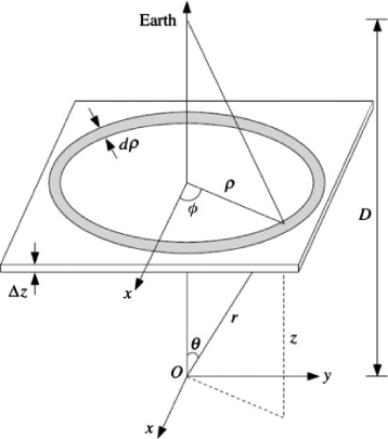
|
(Couderc 1939) can be derived, where t is the time since the explosion was originally observed and c is the speed of light. Then the distance r from the scattering dust to the source event is r2 = ρ2 + z2, and the projected distance on the sky is ρ = (D – z) tan γ, where γ is the angular separation between the source event and the scattering dust.
Measuring ρ through imaging, we can determine the exact three-dimensional location of the scattering dust by simply knowing the time since the outburst occurred and the distance to the object. In the case in which the distance to the object is not well known, the above geometry still provides relative distances between distinct scattering dust locations. Through LE imaging alone, the three-dimensional dust structure in front of an outburst event can be mapped in great detail. While the dust structure can be measured by observing multiple scattering dust locations, it is most thoroughly mapped through monitoring the apparent motion of a given LE system, since the apparent motion is heavily dependent on the scattering dust inclination (see Section 3.3).
3.2 Surface Brightness
The surface brightness of LEs has been derived in different variants by various authors (e.g. Chevalier 1986; Schaefer 1987a; Xu et al. 1994; Sugerman 2003; Patat 2005). Here we follow a derivation of the surface brightness flux fSB by Sugerman (2003) and define
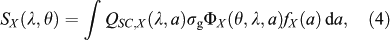
This equation has four principal components: (1) F(λ), the light-curve-weighted integrated event flux of the varying source event, (2) n(r), the dust density as a function of position r, (3) a wavelength-independent spatial component, where Δρ and Δz are the width of the LE on the sky and the depth of the scattering dust sheet along the line of sight, respectively, and (4) the wavelength-dependent integrated scattering function, S(λ, θ), which we describe in more detail in Section 3.2.1.
Note that the event flux F(λ) is the flux difference of the source with respect to its quiescent state. In all the cases where the source event is a one-time transient (e.g. SNe) or where the event is several magnitudes brighter than the magnitude in the quiescent state (e.g. V 838 Mon), this differentiation is not important since the quiescent flux is either zero or close to zero. However, for other objects like Cepheids this is important since what we can detect is the appearing and disappearing scattered flux due to the brightness variation (i.e. the difference in flux between the maximum and minimum brightness) and not the total brightness. For example, we can find scattered light from a non-varying source at a given position, but it is constant with time (i.e. there is no apparent motion of the scattered light) and is commonly called a reflection nebula.
It is important to note that this derivation assumes a photon is only scattered once (single-scattering approximation). However, for very dense dust environments multiple scattering can become important (Chevalier 1986; Patat 2005). The effect that unresolved single and, to an even greater extent, multiple scattered LEs have on the observed colors and spectra of SNe is discussed in detail in Patat et al. (2006).
3.2.1 Dust Scattering
The integrated scattering function S(λ, θ) describes the wavelength-dependent effect of the scattering off dust grains, and is therefore of great importance when calculating the surface brightness of LEs. Here we describe how S can be calculated for our Galaxy and the Magellanic Clouds.
Since different types of dust grains have different integrated scattering functions, they must be added together to get the total integrated scattering function
where X denotes the dust-grain type. Here, X can represent silicon dust grains, carbonaceous dust grains with a neutral polycyclic aromatic hydrocarbon (PAH) component, or carbonaceous dust grains with an ionized PAH component (Weingartner & Draine 2001).
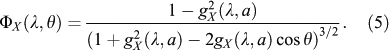
The integrated scattering function SX for a dust grain of type X is
where QX(λ, a) is the dust-grain scattering efficiency and fX(a) is the dust-grain density distribution. The radius of the individual dust grains is given by a, with a grain cross-section σg = πa2. The Henyey–Greenstein phase function, ΦX, is given below, with gX(λ, a) denoting the degree of forward scattering for a given grain (Henyey & Greenstein 1941):
Values for QX and gX(λ, a) can be derived using tables provided by B. T. Draine1 (Draine & Lee 1984; Laor & Draine 1993; Weingartner & Draine 2001; Li & Draine 2001).
We use the ‘MWG’, ‘LMC avg’, and ‘SMC bar’ models defined by Weingartner & Draine (2001), adopting values for their model parameter bC of 5.6 × 10⁻⁵, 2 × 10⁻⁵, and 0, respectively (see tables 1 and 3 of Weingartner & Draine 2001). The models consist of a mixture of carbonaceous grains and amorphous silicate grains. The dust-grain-size distribution is
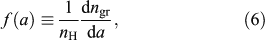
where ngr(a) is the number density of grains smaller than size a and nH is the number density of H nuclei in both atoms and molecules. Note that small carbonaceous grains (a ≤ 10–3 μm) are PAH-like while large carbonaceous grains (a > 10–3 μm) are graphite-like (Li & Draine 2001). The size distributions for carbonaceous dust (fci(a) = Cion f(a) and fcn(a) = (1 – Cion) f(a)) can then be calculated using equations 2, 4, and 6 of Weingartner & Draine (2001). Assuming PAH/graphitic grains to be 50% neutral and 50% ionized (Li & Draine 2001), Cion = 0.5. Equations 5 and 6 are used for amorphous silicate dust, fs.
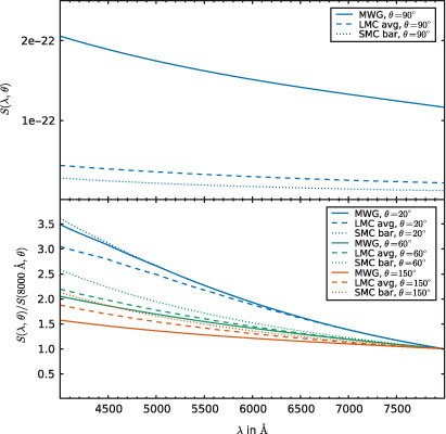
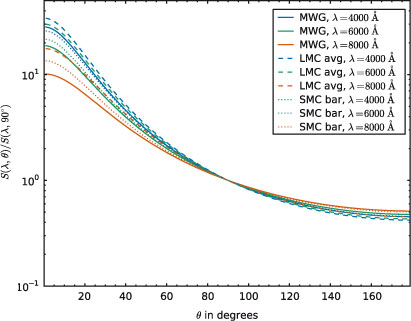
In the upper panel of Figure 2 we show the integrated scattering function S(λ, θ) as a function of wavelength for the Galaxy and Magellanic Cloud models, adopting a scattering angle θ = 90°. In the 4000–8000 Å region shown, the Milky Way Galaxy dust scattering is almost twice as efficient in the blue. For a detailed comparison of the scattering efficiencies, we show in the bottom panel of Figure 2 S(λ, θ) normalized by S(8000 Å, θ) for the three models and various scattering angles. Note that the difference in blueward scattering efficiency is much larger between θ = 20° and 60° than between 60° and 150°. The differences between the models are small but significant, and do not seem to vary significantly with scattering angle. In Figure 3 we show S(λ, θ) on a log scale normalized by S(λ, 90°) for the different models and wavelengths. For scattering angles θ ![]() 60°, the scattering efficiency is quite similar for all models and wavelengths. For θ
60°, the scattering efficiency is quite similar for all models and wavelengths. For θ ![]() 60°, however, the efficiency of blueward scattering is more prominent, with large differences between different models and different wavelengths clearly visible.
60°, however, the efficiency of blueward scattering is more prominent, with large differences between different models and different wavelengths clearly visible.
|
|
3.3 Apparent Motion
One of the most easily measurable properties of LEs is their (often superluminal) apparent proper motion on the sky. The main influences on the apparent motion are the angular separation between the LE and source event, the time since the first light of the source reached Earth, and the distance to the source event (θ, t, and D, respectively). This opens up the possibility that if either one of the age or distance to the event is known then the other parameter can be estimated, since the angular separation can be measured very accurately. However, the apparent motion also depends on the inclination of the scattering dust filament with respect to the line of sight. This fact is often overlooked or ignored, and therefore the derivation of age/distance of the event assumes implicitly or explicitly a certain dust inclination. This can lead to an underestimate of the systematic uncertainty and subsequently to a wrong scientific conclusion. A tale of caution is the analysis by Krause et al. (2005) of the IR echoes of Cas A. Their main scientific conclusion is that most if not all of these IR echoes are caused by a recent X-ray flare of the Cas A SNR based on their apparent motions. However, the analysis was flawed because it did not account for the fact that the apparent motion strongly depends on the inclination of the scattering dust filament (Dwek & Arendt 2008; Rest et al., in preparation).
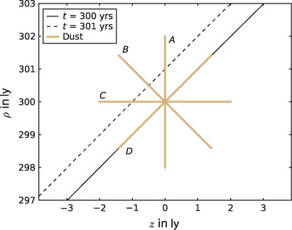
Figure 4 illustrates how different dust sheet inclinations produce different apparent LE motions. We define the inclination angle, α, as the angle of the dust sheet with respect to the ρ axis, where positive angles go from the positive ρ axis towards the negative z axis. The ellipses of equal arrival time defined by Equation 1 are shown as the solid and dashed black line for t = 300 and t = 301 ly, respectively. The dust sheets A, B, C, and D have inclinations of α = 0°, 45°, 90°, and 135°, respectively, crossing the point (z, ρ) = (0, 300) ly (ly denotes units of light years, where 1 ly ~0.3 pc). LEs scattering off dust sheets A, B, C, and D have apparent motions of 1.0c, 0.5c, 0.0c, and ∞, respectively. Here, c is the speed of light. One can see that for dust inclinations in Figure 4 where –45 ≤ α < 0, the apparent motion of the LE is superluminal. Theoretically, for each apparent motion there exists one unique dust filament inclination in a 180° range that produces exactly that apparent motion. For a LE at a given position, there exists degeneracy between the time t since explosion, the dust inclination, and the apparent motion. In order to determine one of these parameters, the other two parameters must be known. However, the inclination of the dust filament is seldom known. A solution is to marginalize over the dust inclination, showing that the apparent motion associated with a dust filament with an inclination perpendicular to the LE ellipsoid is a very good approximation of the expectation value (see Rest et al., in preparation, for a detailed derivation). Note that this marginalization assumes that the inclination of the dust is random, which might not be true due to detection biases. As an example, a common misconception is that for z = 0.0, i.e. when the dust is in the plane of the sky, the apparent motion of LEs is c, implicitly assuming that the dust inclination is α = 0.0°. However, the true expectation value is v = 0.5c associated with α = 45°. As we will see below, the inclination is an important physical property of the scattering dust that affects not only the apparent motion of the LE but also the observed flux profile and spectrum.
|
3.4 Geometric Distance
Under suitable circumstances, LEs provide a unique opportunity to determine the geometric distance to the source object. For a given LE at an angular distance to the source event with known event time, there is still a degeneracy between distance D (source to observer) and the distance z (scattering dust to the source event along the line of sight). This degeneracy gets broken if z can be estimated with some additional information or assumptions.
One of the easiest assumptions to make is z = 0, or that the apparent motion of the LE is the speed of light. However, if these assumptions are not based on any additional evidence, the systematics can be very large and consequently can lead to incorrect distances. Examples for this are discussed for V838 Mon (Section 4.3).
If the geometrical shape of the scattering dust can be constrained, the degeneracy can also be broken. This has been done in the case of SN 1987A where Panagia et al. (1991) determine the distance to the LMC to within a few percent by assuming that its circumstellar ring is circular (Note, however, that they use gaseous emission lines and not scattered LEs, the light-travel delays of which follow similar equations.) Gould (1994) and Gould & Uza (1998) show that the distance changes only at the percent level if the ring is moderately elliptical.
Another complication is added if the source of the LEs has recurrent maxima. In that case it is difficult to determine which LE corresponds to which maximum. If the wrong association is made, catastrophic errors can be the result, and therefore extra care needs to be applied when determining these associations. We discuss two cases in Sections 4.1 and 4.2.
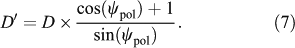
One of the most accurate and robust ways of determining the distance with LEs is using the polarization of the scattered light. The scattering polarizes the light, where the polarization of this scattered light will vary strongly with the scattering angle between the source and the observer (Draine 2003). For normal scattering cross-sections, the angle of maximum polarization, ψpol, is close to 90° and depends only slightly on dust properties like type and grain-size distribution. If the time since the source event, t, is known and ψpol = 90°, the distance to the source event can be calculated with ct = D tan(γ), where γ is the angular separation of the maximum polarization to the source event. In the event that ψpol is not exactly 90° but is known, the method can still be used and the corrected distance is
We refer the reader to Sparks (1994, 1996) who first investigated how this method can be used to determine distances.
Since the maximum polarization angle ψpol depends on the type of scattering dust (usually unknown), systematic uncertainties of the order of 5–10% are introduced into these distance measurements (see figure 5 of Draine 2003). For example, at a wavelength of 6165 Å, ψpol can range from 90°–97° for Small Magellanic Cloud (SMC) bar dust and Galactic dust, respectively. Therefore by determining ψpol at different wavelengths we can verify whether the polarization is consistent with the standard Galactic RV = 3.1 dust model. If the dust is indeed consistent with RV = 3.1, then the theoretical prediction for ψpol is well-constrained and the systematics will be lowered to a few percent.

|
The most important ingredient for this method is to have LEs with scattering angles spread around 90°, which corresponds to having LEs with distances spread around z = 0. The best example in which this method has been applied is V838 Mon, as discussed in Section 4.3, which has an extensive LE system spanning a wide range in z. Not all objects with LEs have such extensive light-echo systems, but Tycho (Rest et al. 2008b), Cas A (Rest et al. 2008b), and most recently η Car (Rest et al. 2012) might have a suitable number of LEs that cover the required range of angular separations from the source event for this method to work.
3.5 LE Profile
The flux profile of a LE is the slice through the LE along the ρ axis pointing toward the source event. This profile is actually the light curve of the source event stretched or compressed depending on the inclination, α, of the scattering dust filament, and convolved with the effects of the dust width, σd, and the seeing (Rest et al. 2011b).
As in Rest et al. (2011b), we illustrate this stretching and compressing effect using a realistic LE scenario similar to that observed in the Cas A echo system. We consider an echo originating from an event in the Galaxy 300 years ago at a distance of 10 000 light years. We assume the outburst event was similar to the observed outburst of SN 1993J. The double-peaked nature of SN 1993J’s light curve makes for a particularly good example to illustrate the observational effects of the scattering dust and the point-spread function (PSF) size. The left panels in Figure 5 show scattering dust filaments (brown-shaded area) of different widths and inclinations. The blue-shaded area indicates a 130-day long event similar to SN 1993J with a fast rise, a peak after 30 days, and a slow decline. Note that the beginning of the outburst is observed at the largest distance away from the source on the sky, not the closest. The scattering dust filaments are located at (z, ρ) = (0, 300) ly with inclinations of α = (0, 0, 0, 45)° and widths of σd = (0.008, 0.03, 0.2, 0.008) ly from top to bottom, respectively. We project the coordinate ρ on to the sky and show on the y-axis the angular difference in ρ to the peak in arcsec.
The middle and right panels of Figure 5 show the LE flux profiles (black lines) for the different dust configurations and PSF sizes. For an infinitely thin dust sheet and an infinitely small PSF, the flux profile is just the projected light curve, as indicated by the red line. For very thin dust filaments (σd = 0.008 ly) with α = 0 and Hubble Space Telescope (HST)-like PSF size, the observed LE profile still shows the signature of the double peak in the light curve (upper middle panel). For ground-based seeing conditions (upper right panel), however, the two peaks are smeared out and indistinguishable. Similarly, if the dust width increases then more and more of the original light-curve shape is lost (σd = 0.03 ly, middle panel in the second row) until not much of the original shape is left (σd = 0.2 ly, middle panel in the third row). Note that the effects of dust width and PSF size are somewhat degenerate.
The effect of the dust-filament inclination is illustrated in the bottom panel, where the LE flux profile is squeezed by a factor of two compared with the profile shown in the top row due to the inclination of the dust filament of α = 45°. Fortunately, the dust-filament inclination is straightforward to determine from the apparent motion if the date of the source event and the distance to it are known (Rest et al. 2011b). A more detailed discussion of the interplay between dust width, dust inclination, and seeing can be found in Rest et al. (2011b). Such accurate modeling of the dust is essential when looking for small differences in spectral features, e.g., when comparing spectra of LEs from the same object as is done in Rest et al. (2011a).
3.6 LE Spectroscopy
While imaging LEs can reveal the nature of the material around an outburst event, and possibly the distance to the event (as in Section 3.4), it is difficult to further our understanding of the outburst itself through imaging. Spectroscopy of LEs, however, allows the outburst to be studied in detail after it has already faded. The first time a spectrum of a LE was taken was in 1902; this was of Nova Persei in a 35-hour effort that can only be called heroic (Perrine 1903). It confirmed that the nebulous moving features seen around Nova Persei were indeed its echoes. Gouiffes et al. (1988) and Suntzeff et al. (1988b) obtained spectra of the inner and outer ring of SN 1987A’s LEs, and compared them with averaged spectra from SN 1987A. They found the LE spectra were most similar to those of the SN near maximum light. Serendipitously, Schmidt et al. (1994) found that 750 days after maximum the spectrum of SN 1991T showed its LE spectrum reflected from foreground dust superimposed on the late-time nebular spectrum. Since 2008, with the work of Rest et al. (2008a), studies using LE spectroscopy have shown it to be a powerful tool to type ancient and historic SNe spectroscopically.
Initial studies assumed that an observed LE spectrum represented a light-curve-weighted integration of the SN spectra at individual epochs (e.g. Rest et al. 2008a; Krause et al. 2008a). In most cases, this is adequate for an approximate spectral identification and classification of the source event. However, Rest et al. (2011b) showed that an observed LE spectrum represents an integration weighted with an effective light curve. The effective light curve can be constructed by applying a window function to the light curve originally observed. Modeling of both astrophysical (dust inclination, scattering, and reddening) and observational (seeing and slit width) effects for a given LE is required to determine the correct window function and therefore interpret the observed (integrated) LE spectrum correctly. This is illustrated in Figure 5: if a slit is placed on the LE profile, in the cases where the width of the dust filament is not very large, the window function is narrow and so the slit probes only a limited part of the source-event epochs (first and second row of panels from the top). Only for very thick dust filaments (third row of panels from the top) is the window function sufficiently wide that the spectrum probes all or nearly all epochs of the source event.
An important part of determining the correct window function is determining whether late-time spectral features are included in the observed LE spectrum. Naively, one might expect that these late-time features are not significant since the surface brightness of the source event has already significantly declined. However, at late times when the spectrum is nebular the observed flux is typically concentrated into a few strong lines. We demonstrate the importance of this late-time contribution using LE spectroscopy from SN 1987A (Rest et al. 2011b). The SN 1987A system is the ideal test-bed for LE spectroscopy, where the high-flux LEs can be paired with the complete spectral and photometric history of the SN as it was originally observed.
Figure 6 shows a modified and updated version of figures 18 and 19 of Rest et al. (2011b), which compares a SN 1987A LE spectrum with its model. The left panel shows the light curve of SN 1987A (Hamuy et al. 1988; Suntzeff et al. 1988a; Hamuy & Suntzeff 1990) and the effective light curve resulting from multiplying the light curve by the appropriate window function. The window function is determined from the best-fitting modeling of the LE profile, taking dust width and inclination, seeing and slit width into account. The necessity of this modeling is clear when comparing model spectra (colored lines) with the observed LE spectrum (black line) in the middle and right panels of Figure 6. The model spectra shown here are integrations of the originally observed spectra of SN 1987A (Menzies et al. 1987; Catchpole et al. 1987, 1988, 1989; Whitelock et al. 1988, 1989; Phillips et al. 1988, 1990) weighted with the effective (orange line) and full (cyan line) light curves shown in the left panel. Here, modeling the correct window function limits the contribution of late-time spectra into the final integrated model spectrum. In the case of SN 1987A, the late-time spectra show strong nebular emission flux in Hα. The Hα line is shown in the right panel of Figure 6, where it is fitted well by the effective light-curve model. Incorrectly modeling the observed LE spectrum using the full light curve of SN 1987A results in an emission component to the Hα line that is far stronger than actually observed in the LE spectrum. It is clear from Figure 6 that detailed consideration of the scattering dust and observational effects is critical in interpreting LE spectra correctly. Examples of LE spectroscopy are discussed in Sections 4.5, 4.6, 4.7, and 4.8.

|
3.7 3D Spectroscopy
LEs offer the exciting opportunity to obtain spectra of the original source event from different lines of sight (LoSs). Figure 7 illustrates how LEs from the Cas A SN, which are scattered by different dust structures, probe the SN from different directions. Observing these arcs is equivalent to observing different hemispheres of the photosphere, providing direct observations of potential asymmetries in the source event. Smith et al. (2003a) first applied this technique, observing the η Car central star from different directions using spectra of the reflection nebula.

|
The signatures of asymmetries in spectra of the same events are much more subtle than when performing spectral classification by comparing different events. Therefore it is essential that both astrophysical (dust inclination, scattering, and reddening) and observational (seeing and slit width) effects are taken into account accurately, as described in the previous Section 3.6 and in more detail in Rest et al. (2011b). An example of 3D spectroscopy is discussed in Section 4.7.
3.8 Spectroscopic Time Series
One as yet unrealized opportunity provided by SN LEs is the ability to obtain a spectral time series of the source event of LEs using very thin scattering dust filaments, as suggested by Rest et al. (2011b). As discussed in Section 3.5, the LE profile is simply the spatially projected light curve of the source event, convolved with the finite thickness of the scattering dust filament and the finite size of the PSF. The spatial extent of the projected light curve is determined by the inclination of the dust filament, in combination with the duration of the event. For short events like SNe and typical dust configurations in our Galaxy, the spatial extent is of the order of arcsec (see Figure 5). This projected light curve is then smeared due to the thickness of the dust filament, in combination with the PSF size. Whether it is possible to resolve the SN spectra temporally depends on the combination of the above parameters.
Figure 5 illustrates this: if the dust filament is very thin, for example as observed for Cas A LEs (Rest et al. 2011b), the resulting window function can have a width of ≈10 days. In the example of SN 1993J, a SN IIb similar to Cas A, it would allow us to observe the spectrum of the shock breakout with an instrument with HST-like PSF size (top and bottom middle panels). An enormous advantage of using LEs for observing the shock break-out is that there is no urgency to obtain observations. Every pixel is a data point, and pixels before the edge of the LE are equivalent to closely spaced non-detections in a SN search. With this method, getting a spectrum at early epochs is as easy (or difficult) as getting a spectrum at late epochs, which is in stark contrast to SN searches, for which it is difficult to obtain spectra at early epochs due to the lag time between when the image is taken, the SN is discovered, and follow-up is triggered.
Spectra at early epochs of a SN or other transients are especially valuable scientifically, since they contain many signatures of the original explosion and also the progenitor. For example, for the shock break-out, the duration, luminosity, and SED depend on a handful of parameters such as the presence of a stellar wind and the ejecta mass (Matzner & McKee 1999), but are most dependent on the progenitor radius (Calzavara & Matzner 2004). The peak brightness of the subsequent fading is dependent on the ejecta mass, kinetic energy, and progenitor radius, while the time-scale for the fading is proportional to both the radius of the photosphere and its temperature (Waxman, Mészáros, & Campana 2007). The ability to resolve the SN spectra temporally allows one to follow the evolution of the explosion, e.g. the evolution of the velocity gradients of spectral features and the abundances of elements in the ejecta (Rest et al. 2011b).
A particularly promising case for this technique is one in which the duration of the source event is very long, since the spatial extent of the projected light curve is proportional to its duration. For example, since the Great Eruption of η Car spanned more than a decade, it is now possible to obtain LE spectra of it from different epochs (Rest et al. 2012), which are only marginally affected by dust width and the PSF size of the observations.
4 LE Case Studies
In recent years, new LEs have been discovered for a variety of events, and new techniques have been used to utilize them. In this section we discuss some of the most prominent LE systems and note the achievements, difficulties, and shortcomings of their analyses (see also Table 1).

|
4.1 S CrA and R CrA
In a recent paper, Ortiz et al. (2010) presented the results of their imaging of LEs around two young stellar objects, the T Tauri star S CrA and the Herbig Ae/Be star R CrA. These classes of variable stars are known for irregular (non-repeating) variability. The authors draw attention to the discovery of the reflection nebulosity and its variation by Hubble (1922) and Lightfoot (1989) although the early works did not interpret their findings as LEs.
The observational material available to Ortiz et al. (2010) for the analysis of S CrA consisted of I-band photometry from the All-Sky Automated Survey (ASAS: Pojmanski 1997) spanning approximately 150 days and nine images spanning 93 days. They adopted a model of a spherically symmetric shell of dust centred on the star and then associated the four brightness peaks from the ASAS time series with the observed LE features from their imaging. Based on their assumptions, they arrived at a distance to S CrA of 128 ± 16 pc and a distance between the star and dust shell of 104 AU. Ortiz et al. (2010) speculated that the dust shell could be similar in nature to the Oort cloud surrounding our Sun.
The major uncertainty in distance estimates using LEs is the scattering geometry, which is unknown without polarization measurements. Distances derived with polarimetry are also subject to systematic errors, as we shall describe in Sections 4.2 and 4.3, even when the dust distribution is described correctly. The analysis of S CrA LEs has several additional flaws. First, given four brightness peaks in four months and nine images spanning three months, it is very likely that there is at least one repeating LE, i.e. one that appears twice, caused by two different peaks scattering off the same dust filament. Second, the brightness differences between the peaks do not seem to be large enough to be able to explain this. Third, there is a large analysis degeneracy between the distance to the star, the times since peak brightness(es), and the distance from the dust to the star. This degeneracy has not yet been fully explored. Finally, the time series itself is noisy and the identification of brightness peaks is not unambiguous. While it may be possible to determine a useful geometric distance to S CrA using LE methods and polarimetry, we conclude that the existing distance estimate is flawed.
4.2 RS Pup
RS Puppis is one of the longest-period and consequently most luminous classical Cepheids known in our Galaxy. As such it is one of the Galactic counterparts of the bright Cepheids used to determine distances to the most distant galaxies amenable to distance estimation with this standard candle. Since Cepheids are believed to be a high-reliability distance indicator, the means to determine an accurate, independent ‘geometric’ distance to RS Puppis, which at a distance of approximately 2.0 kpc cannot be determined by trigonometric parallax with current instrumentation, would be highly desirable.
The reflection nebula of RS Puppis was discovered by Westerlund (1961), who remarked on the possibility of LEs due to the variable nature of the star. Havlen (1972) used a series of photographic images to demonstrate that features within the nebula show light variations at the Cepheid’s pulsation period and argued that these ‘echoes’ could be used to derive a geometric distance, provided that the phase angle of the scattered light was known. More recently, Kervella et al. (2008) obtained an observing season’s worth of high-angular resolution CCD images and used phase-lag measurements of the RS Puppis LEs to estimate a geometric distance of 1992 ± 28 pc, which, if correct, would be by far the most accurate distance to a Cepheid. It would also be a distance unaffected by uncertainty in reddening.
However, Bond & Sparks (2009) showed that the analysis by Kervella et al. (2008) has serious flaws. They pointed out that the implicit assumption by Kervella et al. (2008) that the scattering dust lies, on average, in the plane of the sky is not valid, since the scattering efficiency strongly favors forward scattering and thus significantly biases the results. In addition, Bond & Sparks (2009) showed that the Kervella et al. (2008) results have low statistical significance and argued that with polarization measurements, as demonstrated with V838 Mon by Sparks et al. (2008), the true geometric distance might yet be determined with high precision using this technique.
4.3 V838 Mon
Some of the most spectacular LEs (Henden, Munari, & Schwartz 2002; Bond et al. 2003) appeared when V838 Monocerotis went through an explosion in 2002 (Brown et al. 2002), an outburst so energetic that it became one of the brightest stars in the Local Group for a few weeks in 2002 at MV = –10, gaining nine magnitudes in the V band from its typical quiescent brightness. It ejected so much debris that the material is still not optically thin and it is now thought of as a member of a new class of variables, the so-called intermediate-luminosity red transients.
The echoes around this star were subsequently used to determine its distance. The first attempts using LE expansion measurements greatly underestimated the distance to V838 Mon at <1 kpc (Munari et al. 2002; Kimeswenger et al. 2002), because they were based on the assumption that the LE apparent motion is at the speed of light. More realistic estimates were first done using polarization measurements from HST imaging, setting a lower limit of ≤6 kpc (Bond et al. 2003). A detailed construction of the 3D map of the scattering dust by Tylenda (2004) provided a similar limit of ≤5 kpc, and also indicated that the scattering dust is of interstellar and not circumstellar nature. Assuming that the dust is in a thin sheet, Crause et al. (2005) find a distance of 8.9 ± 1.6 kpc. The most accurate distance determination to date is provided by Sparks et al. (2008), whose detailed analysis of the LE polarization and expansion speed yield a distance of 6.1 ± 0.6 kpc, in very good agreement with other methods (e.g. Afşar & Bond 2007).
The LEs also show a remarkable feature caused by a double helix in the scattering dust filaments, which points almost radially towards V838 Mon (Carlqvist 2005). A possible mechanism for the formation of such a complex structure is the twisting of outflowing material by a magnetic field, as suggested by Carlqvist (2005).
V838 Mon also shows IR echoes (Banerjee et al. 2006), which are spatially coincident with the scattered LEs. The large mass of the dust (>0.2 M⊙) makes it unlikely that the dust is circumstellar and from a previous mass-loss episode, supporting the hypothesis that the dust causing both the scattered and IR echoes is interstellar (Banerjee et al. 2006).
4.4 SN 1987A
Shortly after SN 1987A exploded, spectacular LEs scattered off interstellar dust at distances of ~100 and ~400 pc (Crotts 1988; Suntzeff et al. 1988b; Gouiffes et al. 1988; Couch, Allen, & Malin 1990). Later, LEs scattered off circumstellar dust were also discovered (Crotts, Kunkel, & McCarthy 1989; Bond et al. 1989). These LEs have revealed valuable information about the circumstellar environment around SN 1987A (Sugerman et al. 2005a, b), the interstellar medium (ISM) of the LMC (Xu et al. 1994; Xu, Crotts, & Kunkel 1995; Xu & Crotts 1999), and the asymmetry of SN 1987A itself (Sinnott et al., in preparation).
4.4.1 SN 1987A LEs Scattered off Circumstellar Dust
Crotts & Kunkel (1991) use the LEs within 10 arcsec of SN 1987A to determine the density and 3D structure of the scattering dust, constraining the mass loss of SN 1987A’s progenitor. They find that the scattering dust is consistent with arising from mass lost at a constant rate from a red supergiant atmosphere. Later observations revealed a double-lobed nebula, with a waist that is nearly coincident with the elliptical circumstellar ring seen in atomic recombination lines (Crotts, Kunkel, & Heathcote 1995).
Sugerman et al. (2005a) used LEs detected within 30 arcsec of SN 1987A to construct the most detailed 3D model of the circumstellar environment. They found that a richly structured bipolar nebula surrounds SN 1987A, with an outer, double-lobed ‘peanut’ extending 28 ly along the poles, which is believed to be the contact discontinuity between the red supergiant and main-sequence winds. The waist of this peanut is the ‘Napoleon’s Hat’, which was previously thought to be an independent structure. The innermost circumstellar material is in the form of a cylindrical hourglass, 1 ly in radius and 4 ly long, connected to the peanut by a thick equatorial disk (Sugerman et al. 2005a). With this 3D model of the scattering dust, the progenitor’s mass-loss history can be reconstructed (Sugerman et al. 2005b). They found from the echo fluxes that, from the interior hourglass to the bipolar lobes, the gas density drops from 1–3 to 0.03 cm–3, while the maximum dust-grain size increases from 0.2 to 2 µm and the silicate-to-carbonaceous dust ratio decreases, resulting in a total mass of ~1.7 M⊙. The studies of Sugerman et al. (2005a, b) are the most detailed three-dimensional circumstellar dust reconstruction of any stellar object to date.
4.4.2 SN 1987A LEs Scattered off Interstellar Dust
It is of special interest to understand the structure of the ISM near SN 1987A in the LMC. This is a highly active starburst region with massive stars emitting strong stellar winds. The interaction of these high-energy outflows with the filamentary and spherical structures of the ISM produces bubbles and superbubbles in the region, which trigger additional star formation (e.g. Walborn et al. 1999). LEs from SN 1987A allow the structure of these ISM superbubbles to be traced out in three dimensions.
There are two nearly complete LE rings observed around SN 1987A, caused by two dust sheets roughly perpendicular to the line of sight ~100 and ~400 pc in front of the SN (Crotts 1988; Suntzeff et al. 1988b; Gouiffes et al. 1988; Couch et al. 1990). Xu et al. (1994) found two additional LEs at a much larger distance of ~1000 pc in front of SN 1987A. All of the above LEs were used by Xu et al. (1995) to construct a detailed 3D map of the ISM scattering dust. Comparing this with Hα gas maps, Xu et al. (1995) associate the ring at ~400 pc with reflection from the boundary of the superbubble N157C. They find that the curvature of this dust complex coincides with LH 90, the source of the superbubble. Additionally, the south-eastern arc at a distance of ~1000 pc was found to align with a massive Hα filament discovered by Meaburn, McGee, & Newton (1984). They speculated that these two structures are the near and far sides of a giant superbubble with a diameter of ~600 pc, which itself may have resulted from the merger of several smaller superbubbles.
4.4.3 Asymmetry of SN 1987A
The two main SN 1987A LE rings scattered off interstellar dust (see Section 4.4.2) provide an excellent opportunity to search for spectroscopic asymmetries in SN 1987A using the 3D spectroscopy technique detailed in Section 3.7. These LEs are very bright, allowing the observation of high signal-to-noise ratio spectra. A wealth of previous imaging of the LEs also exists, making the observed apparent motion and hence dust inclination well known. Most importantly, however, the original spectral and photometric history of SN 1987A are both well known, resulting in no ambiguity when modeling the LE spectra (Section 3.6).
Sinnott et al. (in preparation) have obtained spectra of 14 LEs of the inner echo ring of SN 1987A. In order to reduce the effects of nebular and stellar contamination, they have also obtained follow-up sky-only observations at the same position after the LE moved away using the same instrument configuration, for the purpose of difference spectroscopy. In addition to providing multiple viewing angles on to SN 1987A, the LEs that scatter off slightly different dust sheets while probing essentially the same viewing angle allow for a direct observational test of the LE spectra modeling techniques described in Section 3.6. After properly taking the dust-filament extent and inclination into account (see Figure 6), they find evidence for asymmetry along a north-east to south-west axis, with little sign of asymmetry seen in the equatorial east–west directions. The details of this asymmetry will appear in Sinnott et al. (in preparation).
4.5 The 19th-Century Great Eruption of η Carinae
η Car is the most massive and most studied star in our Galaxy. It became the second-brightest star in the sky during its mid-19th century ‘Great Eruption,’ in which it lost more than 10 M⊙ (Smith et al. 2003b). Rest et al. (2012) discovered LEs of the Great Eruption, and subsequent spectroscopic follow-up revealed that its spectral type is most similar to those of G-type supergiants, rather than to F-types or earlier like typical luminous blue variable (LBV) outbursts. This raises doubts that traditional models involving opaque winds explaining LBV outbursts can fully explain the Great Eruption. The absorption lines of the LE spectra indicate that the emitting photosphere has an ejection velocity of ~–200 km s–1 from a viewing angle perpendicular to the principal axis of the Homunculus Nebula (Rest et al. 2012). This is in agreement with velocities predicted by Smith (2006). The η Car LE spectrum also shows a strong asymmetry in the Ca ii IR triplet, extending to a velocity of –850 km s–1 (Rest et al. 2012).
In recent years, some extragalactic non-SN transients (dubbed ‘SN impostors’) have been interpreted as analogues of the Great Eruption of η Car (e.g. Vink 2009), even though the Great Eruption is an extreme case in terms of energy, mass-loss, and duration. It is nevertheless surprising how different the LE spectra of the Great Eruption are compared with those of the SN impostors. Its spectral type is G2–G6, significantly later than all other SN impostors at peak, and it does not show any significant hydrogen or Ca ii IR triplet emission lines (Rest et al. 2012).
4.6 LEs of Ancient SNe in the LMC
The first LEs of ancient or historic SNe were discovered in the LMC by Rest et al. (2005b). They found three LE complexes associated with LMC SNRs: 0509–675, 0519–69.0, and N103B. Using measurements of the LE apparent motions, they determined the ages of these SNRs to be in range 400–800 yr.
A spectrum of one echo associated with SNR 0509–675 reveals that the echo light is from the class of over-luminous Type Ia SNe (Rest et al. 2008a), the first time that an ancient SNe has been typed based on its LE spectrum. This result is in excellent agreement with its classification based on X-ray spectra of SNR 0509–675 (Hughes et al. 1995; Badenes et al. 2008).
Hughes et al. (1995) analyzed X-ray and radio data of the six SNRs in the LMC that have diameters less than 10 pc and are thus presumably the youngest in the LMC. They found three SNRs that have element abundances consistent with nucleosynthesis from Type II SNe, with the remaining three consistent with Type Ia nucleosynthesis. It should be noted that the three SNRs classified as Type Ia are also those SNRs with known LEs. This classification was confirmed for SNR 0509–675 (Rest et al. 2008a) and SNRs 0509–675 and 0519–69.0 (Rest et al., in preparation). Only for the youngest core-collapse SN by far, SN 1987A, were LEs detected. Even though these are low-number statistics, the bias toward detecting LEs from Type Ia SNe can be explained by the fact that core-collapse SNe are typically much fainter than SNe Ia.
4.7 Cas A SN
Cas A is the youngest (~ 330 years old) core-collapse SNR in our Galaxy (Stephenson & Green 2002). Krause et al. (2005) identified features in Spitzer Space Telescope IR images that changed with time. They identified them as IR echoes, which are the result of dust absorbing the SN light, warming and re-radiating it at longer wavelengths. However, their main scientific conclusion that the cause of most if not all of these IR echoes was a series of recent X-ray outbursts from the compact object in the Cas A SNR turned out to be incorrect. They neglected to take into account the fact that the apparent motion depends strongly on the inclination of the scattering dust filament (Dwek & Arendt 2008; see also Section 3.3). Instead, the IR echoes are much more likely caused by the intense and short burst of EUV–UV radiation associated with the shock breakout of the Cas A SN itself (Dwek & Arendt 2008). Kim et al. (2008) used the IR echoes to reconstruct the 3D structure of the absorbing dust filaments.
The first scattered LEs of the Cas A SN were discovered by Rest et al. (2007, 2008b). At the same time, Krause et al. (2008a) followed up spectroscopically one of the IR echoes identified by the Spitzer Space Telescope, and found that the Cas A SN is most similar to the Type IIb SN 1993J. This implies that the progenitor of the Cas A SN was a red supergiant that had lost most of its hydrogen envelope before exploding (Krause et al. 2008a).
Rest et al. (2011a) obtained spectra of Cas A LEs from three different LEs spatially separated by degrees. This means that each of the three spectra views the Cas A SN from a different viewpoint (see Section 3.7). They accounted for the effects of finite dust-filament extent and inclination, and found that the He i λ5876 and Hα features of one LE are blueshifted by an additional ~ 4000 km s–1 relative to the other two LE spectra and to the spectra of SN 1993J, indicating that Cas A was an intrinsically asymmetric SN. Data of the Cas A SNR in the X-ray and the optical also show that there is a dominant Fe-rich outflow in the same direction (Burrows et al. 2005; Wheeler, Maund, & Couch 2008; DeLaney et al. 2010), in excellent agreement with the LE data. This allows, for the first time, structure in the SNR to be directly associated with asymmetry observed in the explosion itself.
4.8 Tycho’s SN
Tycho’s SN of 1572, one of the last two naked-eye SNe in the Galaxy, was classified as Type Ia based on its observed historical light curve and color evolution (Ruiz-Lapuente et al. 2004). Badenes et al. (2006) find that modeling of the X-ray spectra of the Tycho SNR is most consistent with Tycho’s SN being a normal Type Ia, the first time that the subtype of Tycho has been determined, even though only indirectly.
Several LE groups of Tycho’s SN were discovered by Rest et al. (2007, 2008b), who opened the door to allow the spectroscopic classification of this historical SN. Krause et al. (2008b) followed up one of these LEs, and classified the SN as a normal SN Ia by comparing it qualitatively with a small number of SN LE templates constructed from spectrophotometry of nearby SNe, confirming the classification by Badenes et al. (2006). It is noteworthy that Krause et al. (2008b) did not compare the LE spectrum quantitatively with a large set of comparison spectra templates; in particular, they only compare the LE spectrum with a single underluminous SN Ia. Rest et al. (2008a) has shown that even comparing the high signal-to-noise ratio LE templates with themselves only yields conclusive classifications if a large number of templates are available.
5 Conclusions
In the last decade, the number of astrophysical objects with observed LEs has dramatically increased. Newly recognized LEs have been found around extragalactic SNe, as well as LEs from sources in the the Milky Way and Magellanic Clouds. In particular, LEs from nearby sources have proven to be fertile ground for furthering our understanding of transients and variables. The field has advanced from impressive geometric reconstructions of circumstellar and interstellar dust distributions, such as those produced from the study on SN1987A, to the realization of some of the early promise of improved geometric distances. The highly unusual outbursting star V838 Mon had its distance determined to 10% based on polarization measurements of the LEs by determining its geometric distance with an accuracy of better than 10% (Sparks et al. 2008) without any appeal to estimated luminosities of possible counterparts.
An exciting and promising new phase of SN science was ushered in with the discovery of whole LE systems around ancient/historic transients in the LMC and our Galaxy, including Cas A, Tycho, and η Car, where follow-up spectroscopy has allowed the direct comparison of the transient with its remnant. LEs have also now been used, for the first time, to examine transients from the perspectives of their reflection nebulae (scattering dust) and have provided observational spectroscopic constraints on the degree of asymmetry of outbursting objects. One as yet unrealized opportunity provided by LEs is the ability to obtain spectroscopic time series of events and allow the reconstruction of the originally unobserved light-curve shapes of SNe.
There is a great deal of discovery space left in LE research, since only a small fraction of the sky has been searched for time-variable, low-surface-brightness, non-stellar features. As currently envisaged, the next generation of wide-field, time-domain surveys like Pan-STARRS (Kaiser et al. 2010), PTF (Rau et al. 2009), Skymapper (Keller et al. 2007), and ultimately LSST (Ivezic et al. 2008) is being designed to study the celestial sphere based dominantly on the variability of point sources. A mode in which whole images of the sky are preserved with a cadence of weeks or months is likely to reveal an abundance of additional LE features and the history and perspectives they carry in their scattered light.
Acknowledgments
We thank M. Bode for bringing the Nova Persei LE spectrum to our attention. DW acknowledges the support of a Discovery Grant from the Natural Sciences and Engineering Research Council of Canada (NSERC).
References
Afşar, M. and Bond, H. E., 2007, AJ, 133, 387Alard, C., 2000, A&AS, 144, 363
Alard, C. and Lupton, R. H., 1998, ApJ, 503, 325
| Crossref | GoogleScholarGoogle Scholar |
Andrews, J. E. et al., 2011, ApJ, 731, 47
| Crossref | GoogleScholarGoogle Scholar |
Badenes, C., Borkowski, K. J., Hughes, J. P., Hwang, U. and Bravo, E., 2006, ApJ, 645, 1373
| Crossref | GoogleScholarGoogle Scholar | 1:CAS:528:DC%2BD28XotVers70%3D&md5=63919bec043ab812bd8f20ba75bc23f2CAS |
Badenes, C., Hughes, J. P., Cassam-Chenaï, G. and Bravo, E., 2008, ApJ, 680, 1149
| Crossref | GoogleScholarGoogle Scholar | 1:CAS:528:DC%2BD1cXos1yms7s%3D&md5=e9ef011e9da13d8d9df1fef3a6ba25d8CAS |
Banerjee, D. P. K., Su, K. Y. L., Misselt, K. A. and Ashok, N. M., 2006, ApJL, 644, L57
| Crossref | GoogleScholarGoogle Scholar |
Barris, B. J., Tonry, J. L., Novicki, M. C. and Wood-Vasey, W. M., 2005, AJ, 130, 2272
Bode, M. F. and Evans, A., 1980a, A&A, 89, 158
| 1:CAS:528:DyaL3cXlslKqtL4%3D&md5=ff3321576def681dfe9a35f1f23ba021CAS |
Bode, M. F. and Evans, A., 1980b, MNRAS, 193, 21P
Bode, M. F. and Evans, A., 1985, A&A, 151, 452
Bode, M. F., O'Brien, T. J. and Simpson, M., 2004, ApJL, 600, L63
| Crossref | GoogleScholarGoogle Scholar | 1:CAS:528:DC%2BD2cXhsVSgsbc%3D&md5=a217812c28ca9deb19296826a729a2c0CAS |
Boffi, F. R., Sparks, W. B. and Macchetto, F. D., 1999, A&AS, 138, 253
Bond, H. E. and Sparks, W. B., 2009, A&A, 495, 371
Bond, H. E., Panagia, N., Gilmozzi, R. and Meakes, M., 1989, IAUC, 4733, 1
Bond, H. E. et al., 2003, Natur, 422, 405
| Crossref | GoogleScholarGoogle Scholar | 1:CAS:528:DC%2BD3sXitlGgtbo%3D&md5=9c4cafb1fde300608dcabf265fa151eeCAS |
Brown, N. J., Waagen, E. O., Scovil, C., Nelson, P., Oksanen, A., Solonen, J. and Price, A., 2002, IAUC, 7785, 1
Burrows, A., Walder, R., Ott, C. D. & Livne, E., 2005, in ASP Conf. Ser. 332, The Fate of the Most Massive Stars, ed. R. Humphreys & K. Stanek (San Francisco: ASP), 350
Calzavara, A. J. and Matzner, C. D., 2004, MNRAS, 351, 694
| Crossref | GoogleScholarGoogle Scholar | 1:CAS:528:DC%2BD2cXms1ygt74%3D&md5=1d19e53e640f21c46a5b4b241cf3fbf4CAS |
Cappellaro, E. et al., 2001, ApJL, 549, L215
| Crossref | GoogleScholarGoogle Scholar |
Carlqvist, P., 2005, A&A, 436, 231
| 1:CAS:528:DC%2BD2MXlvFKmurY%3D&md5=089ac368e30fa0bc58cf814f3f289e71CAS |
Catchpole, R. M. et al., 1987, MNRAS, 229, 15P
| 1:CAS:528:DyaL2sXmsVKjt70%3D&md5=dd44cc774562f3eb167c6509be39dca6CAS |
Catchpole, R. M. et al., 1988, MNRAS, 231, 75P
| 1:CAS:528:DyaL1cXitFeht7o%3D&md5=55543630ea4e1c796c4149fc5ccf03d2CAS |
Catchpole, R. M. et al., 1989, MNRAS, 237, 55P
| 1:CAS:528:DyaL1MXhvVahtLY%3D&md5=99f3d8e32792a6363bdb1d96a995f05fCAS |
Chevalier, R. A., 1986, ApJ, 308, 225
| Crossref | GoogleScholarGoogle Scholar | 1:CAS:528:DyaL28Xls1Wlsro%3D&md5=d58500e25870ba37628310390d521f45CAS |
Chugai, N. N., 1992, SvA, 36, 63
Couch, W. J., Allen, D. A. and Malin, D. F., 1990, MNRAS, 242, 555
Couderc, P., 1939, AnAp, 2, 271
Crause, L. A., Lawson, W. A., Menzies, J. W. and Marang, F., 2005, MNRAS, 358, 1352
| Crossref | GoogleScholarGoogle Scholar |
Crotts, A., 1988, IAUC, 4561, 4
Crotts, A. P. S. and Kunkel, W. E., 1991, ApJL, 366, L73
| Crossref | GoogleScholarGoogle Scholar | 1:CAS:528:DyaK3MXhslChu7c%3D&md5=92a759e896f3c0b1330df5bb77764d05CAS |
Crotts, A. P. S. and Yourdon, D., 2008, ApJ, 689, 1186
| Crossref | GoogleScholarGoogle Scholar |
Crotts, A. P. S., Kunkel, W. E. and McCarthy, P. J., 1989, ApJL, 347, L61
| Crossref | GoogleScholarGoogle Scholar | 1:CAS:528:DyaK3cXms1SmsA%3D%3D&md5=0f118438883cd66b5c0f9f1c99373d38CAS |
Crotts, A. P. S., Kunkel, W. E. and Heathcote, S. R., 1995, ApJ, 438, 724
| Crossref | GoogleScholarGoogle Scholar |
DeLaney, T. et al., 2010, ApJ, 725, 2038
| Crossref | GoogleScholarGoogle Scholar | 1:CAS:528:DC%2BC3MXms1Wmtw%3D%3D&md5=da362dedf48a78ff9be7594453fd4082CAS |
Di Carlo, E. et al., 2002, ApJ, 573, 144
| Crossref | GoogleScholarGoogle Scholar | 1:CAS:528:DC%2BD38XlvVSgsL4%3D&md5=f89b8dd2ebd61deb80501f6a258c4382CAS |
Draine, B. T., 2003, ApJ, 598, 1017
| Crossref | GoogleScholarGoogle Scholar | 1:CAS:528:DC%2BD2cXjvVWrsw%3D%3D&md5=68522afd4fb52b9936e4b99de824f660CAS |
Draine, B. T. and Lee, H. M., 1984, ApJ, 285, 89
| Crossref | GoogleScholarGoogle Scholar | 1:CAS:528:DyaL2cXmtF2itbo%3D&md5=9d217ea5cde0064424768d594669bf9dCAS |
Dwek, E., 1983, ApJ, 274, 175
| Crossref | GoogleScholarGoogle Scholar | 1:CAS:528:DyaL3sXmt1Wruro%3D&md5=30c06dae65a8f92f618eff05d26d59e2CAS |
Dwek, E. and Arendt, R. G., 2008, ApJ, 685, 976
| Crossref | GoogleScholarGoogle Scholar | 1:CAS:528:DC%2BD1cXht1KqtbfP&md5=615254e50b781b6b1bf8e5ec097f0a76CAS |
Gallagher, J. S. et al., 2011, BAAS, 43, 337.22
Garnavich, P. M. et al., 2001, BAAS, 33, 1370
Gehrz, R. D., 1988, ARA&A, 26, 377
| Crossref | GoogleScholarGoogle Scholar | 1:CAS:528:DyaL1cXmtl2gtrs%3D&md5=43f5971d4d79ebe674553cd72fd6c5bcCAS |
Gouiffes, C. et al., 1988, A&A, 198, L9
| 1:CAS:528:DyaL1cXmtl2qt7s%3D&md5=efcd890e34125a99f4ecfc01828a1700CAS |
Gould, A., 1994, ApJ, 425, 51
| Crossref | GoogleScholarGoogle Scholar | 1:CAS:528:DyaK2cXlvFSnsLw%3D&md5=2a7bd3c51b08f2365729b6180ca515d0CAS |
Gould, A. and Uza, O., 1998, ApJ, 494, 118
| Crossref | GoogleScholarGoogle Scholar | 1:CAS:528:DyaK1cXhs1Wntb0%3D&md5=a112b5774f693c7afd3ff77c8244186fCAS |
Hamuy, M. and Suntzeff, N. B., 1990, AJ, 99, 1146
Hamuy, M., Suntzeff, N. B., Gonzalez, R. and Martin, G., 1988, AJ, 95, 63
Havlen, R. J., 1972, A&A, 16, 252
Henden, A., Munari, U. and Schwartz, M., 2002, IAUC, 7859, 1
Henyey, L. C. and Greenstein, J. L., 1941, ApJ, 93, 70
| Crossref | GoogleScholarGoogle Scholar |
Hubble, E., 1922, CMWCI, 250, 1
Hughes, J. P. et al., 1995, ApJL, 444, L81
| Crossref | GoogleScholarGoogle Scholar | 1:CAS:528:DyaK2MXmtFGksbw%3D&md5=1f31bd49c40bf31677bc6a1fa2f49c00CAS |
Ivezic, Z., et al., 2008, ArXiv e-print (0805.2366)
Kaiser, N., et al., 2010, in Society of Photo-Optical Instrumentation Engineers (SPIE) Conference Vol. 7733, The Pan-STARRS Wide-Field Optical/NIR Imaging Survey, ed. L. M. Stepp, R. Gilmozzi & H. J. Hall, 77330E
Kapteyn, J. C., 1902, AN, 157, 201
Keller, S. C. et al., 2007, PASA, 24, 1
| Crossref | GoogleScholarGoogle Scholar |
Kervella, P., Mérand, A., Szabados, L., Fouqué, P., Bersier, D., Pompei, E. and Perrin, G., 2008, A&A, 480, 167
Kim, Y., Rieke, G. H., Krause, O., Misselt, K., Indebetouw, R. & Johnson, K. E., 2008, ApJ, in press
Kimeswenger, S., Lederle, C., Schmeja, S. and Armsdorfer, B., 2002, MNRAS, 336, L43
| Crossref | GoogleScholarGoogle Scholar |
Kotak, R. et al., 2009, ApJ, 704, 306
| Crossref | GoogleScholarGoogle Scholar | 1:CAS:528:DC%2BD1MXhtl2ksrrF&md5=b4d4045b32f572c25f42d33557351f7aCAS |
Krause, O. et al., 2005, Sci, 308, 1604
| Crossref | GoogleScholarGoogle Scholar | 1:CAS:528:DC%2BD2MXltFems7g%3D&md5=10035ec48ba26d553ac9438ba14f0292CAS |
Krause, O., Birkmann, S. M., Usuda, T., Hattori, T., Goto, M., Rieke, G. H. and Misselt, K. A., 2008a, Sci, 320, 1195
| Crossref | GoogleScholarGoogle Scholar | 1:CAS:528:DC%2BD1cXmt1Oju7Y%3D&md5=a03883ecca0c37258c104abd3c028a74CAS |
Krause, O., Tanaka, M., Usuda, T., Hattori, T., Goto, M., Birkmann, S. and Nomoto, K., 2008b, Natur, 456, 617
| Crossref | GoogleScholarGoogle Scholar | 1:CAS:528:DC%2BD1cXhsVGlur7O&md5=111e071702d6226c1a1919caa147fd2dCAS |
Laor, A. and Draine, B. T., 1993, ApJ, 402, 441
| Crossref | GoogleScholarGoogle Scholar |
Li, A. and Draine, B. T., 2001, ApJ, 554, 778
| Crossref | GoogleScholarGoogle Scholar | 1:CAS:528:DC%2BD3MXlslGkurg%3D&md5=75d0bafab8aed568cc16eca51d1c8671CAS |
Lightfoot, J. F., 1989, MNRAS, 239, 665
Lintott, C. J. et al., 2009, MNRAS, 399, 129
| Crossref | GoogleScholarGoogle Scholar | 1:CAS:528:DC%2BD1MXhtlygtLnI&md5=2ec729a5bce1146fd15b827317a8e5c6CAS |
Liu, J.-F., Bregman, J. N. and Seitzer, P., 2003, ApJ, 582, 919
| Crossref | GoogleScholarGoogle Scholar |
Maslov, I. A., 2000, AstL, 26, 428
Matzner, C. D. and McKee, C. F., 1999, ApJ, 510, 379
| Crossref | GoogleScholarGoogle Scholar | 1:CAS:528:DyaK1MXhtFSkurw%3D&md5=6a9ef8ab3c196054d4b2106a86b4ea89CAS |
Meaburn, J., McGee, R. X. and Newton, L. M., 1984, MNRAS, 206, 705
| 1:CAS:528:DyaL2cXhtFWktrk%3D&md5=f067718bab19041ee93731e6db9271cfCAS |
Menzies, J. W. et al., 1987, MNRAS, 227, 39P
| 1:CAS:528:DyaL2sXlt1eqs7o%3D&md5=f8390452c84af2c3dc5f56c1e864ad73CAS |
Miller, A. A., Smith, N., Li, W., Bloom, J. S., Chornock, R., Filippenko, A. V. and Prochaska, J. X., 2010, AJ, 139, 2218
| 1:CAS:528:DC%2BC3cXotVaksrw%3D&md5=e7e44fa9b4a09624d51cb3b85bd3880aCAS |
Munari, U. et al., 2002, A&A, 389, L51
| 1:CAS:528:DC%2BD38Xmtlaht7k%3D&md5=f051fb1219705e2e521381658704f985CAS |
Newman, A. B. and Rest, A., 2006, PASP, 118, 1484
| Crossref | GoogleScholarGoogle Scholar |
Ortiz, J. L., Sugerman, B. E. K., de La Cueva, I., Santos-Sanz, P., Duffard, R, Gil-Hutton, R, Melita, M and Morales, N, 2010, A&A, 519, A7
Otsuka, M. et al., 2012, ApJ, 744, 26
| Crossref | GoogleScholarGoogle Scholar |
Panagia, N., Gilmozzi, R., Macchetto, F., Adorf, H.-M. and Kirshner, R. P., 1991, ApJL, 380, L23
| Crossref | GoogleScholarGoogle Scholar | 1:CAS:528:DyaK3MXms1Kjs7k%3D&md5=d9eecb87e98cdc875203ca47ba04df3cCAS |
Patat, F., 2005, MNRAS, 357, 1161
| Crossref | GoogleScholarGoogle Scholar |
Patat, F., Benetti, S., Cappellaro, E. and Turatto, M., 2006, MNRAS, 369, 1949
| Crossref | GoogleScholarGoogle Scholar |
Perrine, C. D., 1903, ApJ, 17, 310
| Crossref | GoogleScholarGoogle Scholar |
Phillips, M. M., Heathcote, S. R., Hamuy, M. and Navarrete, M., 1988, AJ, 95, 1087
| 1:CAS:528:DyaL1cXitFehs7k%3D&md5=8e331977d6948e1e64eaba617d6822a4CAS |
Phillips, M. M., Hamuy, M., Heathcote, S. R., Suntzeff, N. B. and Kirhakos, S., 1990, AJ, 99, 1133
| 1:CAS:528:DyaK3cXitVOitLc%3D&md5=c3c03c1657c2c563b0db44d17a373c67CAS |
Pojmanski, G., 1997, AcA, 47, 467
Quinn, J. L., Garnavich, P. M., Li, W., Panagia, N., Riess, A., Schmidt, B. P. and Della Valle, M., 2006, ApJ, 652, 512
| Crossref | GoogleScholarGoogle Scholar |
Rampadarath, H. et al., 2010, A&A, 517, L8
Rau, A. et al., 2009, PASP, 121, 1334
| Crossref | GoogleScholarGoogle Scholar |
Rest, A. et al., 2005a, ApJ, 634, 1103
| Crossref | GoogleScholarGoogle Scholar |
Rest, A. et al., 2005b, Natur, 438, 1132
| Crossref | GoogleScholarGoogle Scholar | 1:CAS:528:DC%2BD2MXhtlakurrM&md5=1ad4b869ee9f09985a3bc9e9b0d812bcCAS |
Rest, A. et al., 2007, BAAS, 38, 935
Rest, A. et al., 2008a, ApJ, 680, 1137
| Crossref | GoogleScholarGoogle Scholar |
Rest, A. et al., 2008b, ApJL, 681, L81
| Crossref | GoogleScholarGoogle Scholar | 1:CAS:528:DC%2BD1cXps1Sltb8%3D&md5=0ec32327edf58a115f6f3622d0682adaCAS |
Rest, A. et al., 2011a, ApJ, 732, 3
| Crossref | GoogleScholarGoogle Scholar |
Rest, A., Sinnott, B., Welch, D. L., Foley, R. J., Narayan, G., Mandel, K., Huber, M. E. and Blondin, S., 2011b, ApJ, 732, 2
| Crossref | GoogleScholarGoogle Scholar |
Rest, A. et al., 2012, Natur, 482, 375
| Crossref | GoogleScholarGoogle Scholar | 1:CAS:528:DC%2BC38Xit12jtbc%3D&md5=5bc5bd885dee89e04d71e55c7d3ac4a1CAS |
Ritchey, G. W., 1901a, ApJ, 14, 293
| Crossref | GoogleScholarGoogle Scholar |
Ritchey, G. W., 1901b, ApJ, 14, 167
| Crossref | GoogleScholarGoogle Scholar |
Ritchey, G. W., 1902, ApJ, 15, 129
| Crossref | GoogleScholarGoogle Scholar |
Romaniello, M., Patat, F., Panagia, N., Sparks, W. B., Gilmozzi, R. and Spyromilio, J., 2005, ApJ, 629, 250
| Crossref | GoogleScholarGoogle Scholar | 1:CAS:528:DC%2BD2MXhtVehurjN&md5=077a91a7a4c06d36601d0c79076de0c9CAS |
Roscherr, B. and Schaefer, B. E., 2000, ApJ, 532, 415
| Crossref | GoogleScholarGoogle Scholar |
Ruiz-Lapuente, P. et al., 2004, Natur, 431, 1069
| Crossref | GoogleScholarGoogle Scholar | 1:CAS:528:DC%2BD2cXovFGntr0%3D&md5=95ae931e1d63a1fc46a6c70101b19193CAS |
Schaefer, B. E., 1987a, ApJL, 323, L47
| Crossref | GoogleScholarGoogle Scholar |
Schaefer, B. E., 1987b, ApJL, 323, L51
| Crossref | GoogleScholarGoogle Scholar |
Schaefer, B. E., 1988, ApJ, 327, 347
| Crossref | GoogleScholarGoogle Scholar |
Schmidt, B. P., Kirshner, R. P., Leibundgut, B., Wells, L. A., Porter, A. C., Ruiz-Lapuente, P., Challis, P. and Filippenko, A. V., 1994, ApJL, 434, L19
| Crossref | GoogleScholarGoogle Scholar | 1:CAS:528:DyaK2MXitFaju7c%3D&md5=31493ad527353ad422b73c14dd11a01eCAS |
Seaquist, E. R., Bode, M. F., Frail, D. A., Roberts, J. A., Evans, A. and Albinson, J. S., 1989, ApJ, 344, 805
| Crossref | GoogleScholarGoogle Scholar | 1:CAS:528:DyaL1MXlvVemur0%3D&md5=7f3e54db58cd246fe5aa4c95bbc2db7fCAS |
Shklovskii, I. S., 1964, Astron. Circ. USSR, , 306
Smith, N., 2006, ApJ, 644, 1151
| Crossref | GoogleScholarGoogle Scholar | 1:CAS:528:DC%2BD28Xnt1CqtLw%3D&md5=319a1ebf66d423bb25c7f2f95ad245c2CAS |
Smith, N., Davidson, K., Gull, T. R., Ishibashi, K. and Hillier, D. J., 2003a, ApJ, 586, 432
| Crossref | GoogleScholarGoogle Scholar | 1:CAS:528:DC%2BD3sXjtVeku7Y%3D&md5=709d203c98eb6809c07cd29a7cf619baCAS |
Smith, N., Gehrz, R. D., Hinz, P. M., Hoffmann, W. F., Hora, J. L., Mamajek, E. E. and Meyer, M. R., 2003b, AJ, 125, 1458
Sparks, W. B., 1994, ApJ, 433, 19
| Crossref | GoogleScholarGoogle Scholar |
Sparks, W. B., 1996, ApJ, 470, 195
| Crossref | GoogleScholarGoogle Scholar |
Sparks, W. B., Macchetto, F., Panagia, N., Boffi, F. R., Branch, D., Hazen, M. L. and della Valle, M., 1999, ApJ, 523, 585
| Crossref | GoogleScholarGoogle Scholar |
Sparks, W. B. et al., 2008, AJ, 135, 605
Stephenson, F. R. & Green, D. A., 2002, Historical Supernovae and their Remnants, International Series in Astronomy and Astrophysics, Vol. 5 (Oxford: Clarendon Press)
Sugerman, B. E. K., 2003, AJ, 126, 1939
Sugerman, B. E. K., 2005, ApJL, 632, L17
| Crossref | GoogleScholarGoogle Scholar |
Sugerman, B. E. K. and Crotts, A. P. S., 2002, ApJL, 581, L97
| Crossref | GoogleScholarGoogle Scholar |
Sugerman, B. E. K., Crotts, A. P. S., Kunkel, W. E., Heathcote, S. R. and Lawrence, S. S., 2005a, ApJ, 627, 888
| Crossref | GoogleScholarGoogle Scholar | 1:CAS:528:DC%2BD2MXnsVChsbs%3D&md5=e27b4d7662168dd1034e3b0c635f61a5CAS |
Sugerman, B. E. K., Crotts, A. P. S., Kunkel, W. E., Heathcote, S. R. and Lawrence, S. S., 2005b, ApJS, 159, 60
| Crossref | GoogleScholarGoogle Scholar |
Sugerman, B. E. K., et al., 2012, ArXiv e-print (1202.3075)
Suntzeff, N. B., Hamuy, M., Martin, G., Gomez, A. and Gonzalez, R., 1988a, AJ, 96, 1864
| 1:CAS:528:DyaL1MXms1aqsQ%3D%3D&md5=3d1f9e9bd76f7cfa290fd7a827377c7fCAS |
Suntzeff, N. B., Heathcote, S., Weller, W. G., Caldwell, N. and Huchra, J. P., 1988b, Natur, 334, 135
| Crossref | GoogleScholarGoogle Scholar |
Swope, H. H., 1940, BHarO, 913, 11
Tomaney, A. B. and Crotts, A. P. S., 1996, AJ, 112, 2872
Tylenda, R., 2004, A&A, 414, 223
van den Bergh, S., 1965a, AJ, 70, 667
van den Bergh, S., 1965b, PASP, 77, 269
| Crossref | GoogleScholarGoogle Scholar |
van den Bergh, S., 1966, PASP, 78, 74
| Crossref | GoogleScholarGoogle Scholar |
van den Bergh, S., 1977, PASP, 89, 637
| Crossref | GoogleScholarGoogle Scholar |
Van Dyk, S. D., Li, W. and Filippenko, A. V., 2006, PASP, 118, 351
| Crossref | GoogleScholarGoogle Scholar |
Vink, J. S., 2009, ArXiv e-print (0905.3338)
Walborn, N. R., Barbá, R. H., Brandner, W, Rubio, M, Grebel, E. K. and Probst, R. G., 1999, AJ, 117, 225
| 1:CAS:528:DyaK1MXht1Cqsro%3D&md5=bd3e1d8fa9887d5e9f85c00092373935CAS |
Wang, X., Li, W., Filippenko, A. V., Foley, R. J., Smith, N. and Wang, L., 2008, ApJ, 677, 1060
| Crossref | GoogleScholarGoogle Scholar | 1:CAS:528:DC%2BD1cXmtFKisrc%3D&md5=a16ff583963cc3a5b63ea10bc00c1db1CAS |
Waxman, E., Mészáros, P. and Campana, S., 2007, ApJ, 667, 351
| Crossref | GoogleScholarGoogle Scholar |
Weingartner, J. C. and Draine, B. T., 2001, ApJ, 548, 296
| Crossref | GoogleScholarGoogle Scholar |
Welch, D. L. et al., 2007, ApJ, 669, 525
| Crossref | GoogleScholarGoogle Scholar | 1:CAS:528:DC%2BD2sXhtlektb3K&md5=ae0eac4adad7385b58cc6265610b943cCAS |
Westerlund, B., 1961, PASP, 73, 72
| Crossref | GoogleScholarGoogle Scholar |
Wheeler, J. C., Maund, J. R. and Couch, S. M., 2008, ApJ, 677, 1091
| Crossref | GoogleScholarGoogle Scholar | 1:CAS:528:DC%2BD1cXmtFKis70%3D&md5=10a3832ae75380fddae9db3a18cb8193CAS |
Whitelock, P. A. et al., 1988, MNRAS, 234, 5P
| 1:CAS:528:DyaL1cXmtVSnu78%3D&md5=8dddb838e63146039a9ebe3baf4d9f27CAS |
Whitelock, P. A. et al., 1989, MNRAS, 240, 7P
| 1:CAS:528:DyaL1MXmtVClu7c%3D&md5=04936cf57973ce4aba1a2d8238176359CAS |
Xu, J. and Crotts, A. P. S., 1999, ApJ, 511, 262
| Crossref | GoogleScholarGoogle Scholar | 1:CAS:528:DyaK1MXhvVOnsro%3D&md5=75cd6ab456325c7807f2a4476d7e7a6aCAS |
Xu, J., Crotts, A. P. S. and Kunkel, W. E., 1994, ApJ, 435, 274
| Crossref | GoogleScholarGoogle Scholar |
Xu, J., Crotts, A. P. S. and Kunkel, W. E., 1995, ApJ, 451, 806
| Crossref | GoogleScholarGoogle Scholar |
Zwicky, F., 1940, RvMP, 12, 66
1 http://www.astro.princeton.edu/~draine/dust/dust.diel.html