
Comparison of Potential ASKAP Hi Survey Source Finders
A. Popping A E , R. Jurek B , T. Westmeier A , P. Serra A , L. Flöer D , M. Meyer A and B. Koribalski BA International Centre for Radio Astronomy Research (ICRAR), The University of Western Australia, 35 Stirling Hwy, Crawley, WA 6009, Australia
B Australia Telescope National Facility, CSIRO Astronomy and Space Science, PO Box 76, Epping, NSW 1710, Australia
C Netherlands Institute for Radio Astronomy (ASTRON), Postbus 2, 7990 AA Dwingeloo, The Netherlands
D Argelander-Institut für Astronomie, Auf dem Hügel 71, 53121 Bonn, Germany
E Corresponding author. Email: attila.popping@icrar.org
Publications of the Astronomical Society of Australia 29(3) 318-339 https://doi.org/10.1071/AS11067
Submitted: 8 November 2011 Accepted: 19 January 2012 Published: 24 February 2012
Journal Compilation © Astronomical Society of Australia 2012
Abstract
The large size of the ASKAP Hi surveys DINGO and WALLABY necessitates automated 3D source finding. A performance difference of a few percent corresponds to a significant number of galaxies being detected or undetected. As such, the performance of the automated source finding is of paramount importance to both of these surveys. We have analysed the performance of various source finders to determine which will allow us to meet our survey goals during the DINGO and WALLABY design studies. Here we present a comparison of the performance of five different methods of automated source finding. These source finders are duchamp, gamma-finder, a cnhi finder, a 2d–1d wavelet reconstruction finder and a sigma clipping method (s+c finder). Each source finder was applied to the same three-dimensional data cubes containing (a) point sources with a Gaussian velocity profile and (b) spatially extended model-galaxies with inclinations and rotation profiles. We focus on the completeness and reliability of each algorithm when comparing the performance of the different source finders.
Keywords: methods: data analysis
1 Introduction
Radio astronomy is facing a new era, acquiring extremely large data volumes with the coming of the Square Kilometre Array (SKA; Dewdney et al. 2009) and precursors such as MeerKAT (Jonas 2009) in South Africa, APERTIF (Verheijen et al. 2008) in the Netherlands and the Australian SKA Pathfinder (ASKAP) (DeBoer et al. 2009) in Australia. Various continuum (2D) and spectral line (3D) surveys, which cover large fractions of the sky, will be conducted with these telescopes. The surveys are expected to detect millions of objects, accelerating the need for reliable automated source finders.
A good source finder should have high completeness and high reliability, i.e. a low rate of false detections. Choosing a suitable trade-off between both parameters is necessary and depends on both the algorithm and the rms uniformity of the data. Detecting objects is relatively easy in the case of (strong) point sources, but becomes more complicated in the case of irregular shapes and diffuse or extended emission in one or more dimensions and at low signal to noise ratios. The work presented in this paper aims to highlight the strengths and weaknesses of potential 3D source finders for the Deep Investigations of Neutral Gas Origins (DINGO) survey (Meyer 2009) and the Widefield ASKAP L-Band Legacy All-Sky Blind Survey (WALLABY) (Koribalski & Staveley-Smith 2009). These are two of the large Hi survey science projects for ASKAP (Johnston et al. 2008). To achieve the respective science goals, we aim to develop source finding algorithms which reliably and efficiently recover 3D Hi sources.
We have identified five different source finders that will be subjected to testing and comparison: 1) the duchamp source finder (Whiting 2011), 2) gamma-finder (Boyce 2003), 3) the cnhi source finder (Jurek 2012), 4) the 2d–1d wavelet reconstruction source finder (Flöer & Winkel 2012) and 5) the s+c finder (Serra et al. 2011).
Testing of each algorithm was done on the same set of data cubes. The first containing 961 point sources with varying peak flux and a Gaussian velocity profile. The second cube contains 1024 modelled galaxies with more realistic properties such as extended disks, inclinations and rotation profiles. Here we compare their performance in terms of completeness and reliability.
In Section 2 we briefly summarise the main properties of the source finding algorithms and in Section 3 we describe the testing method and the two model cubes that have been used for the testing. The test results are presented in Section 4, followed by a discussion in Section 5. We compare in detail the performance and reliability of the source finders, to understand where the strong and weak points of the different source finders are and to highlight possible improvements. We finish with a short conclusion in the final section.
2 Source Finders
Here we provide a short description of the five source finders compared throughout the paper. For a more extended review of the individual algorithm we refer to the reference papers describing each method in detail.
2.1 duchamp
duchamp (Whiting 2011) is a source finder designed for 3D data, although it can be used for 2D and even 1D datasets. The source finder has been developed by Matthew Whiting at CSIRO.1 duchamp identifies sources by simply applying a specified flux or signal-to-noise threshold and searching for signals above that threshold. In a second step, detections are merged or rejected based on several criteria specified by the user. To improve its performance, duchamp offers several methods of preconditioning and filtering of the input data, including spatial and spectral smoothing as well as wavelet reconstruction of the entire image or cube. In a final step, duchamp measures several basic parameters for each detected source, including position, radial velocity, size, line width, and integrated flux. The performance of the duchamp source finder is tested in Westmeier, Popping & Serra (2012).
2.2 cnhi Source Finder
The Characterised Noise Hi (cnhi) source finder (Jurek 2012) is being developed as part of the WALLABY design study. The cnhi source finder treats spectral datacubes as a collection of spectra, using the Kuiper test, which is a variant of the Kolmogorov-Smirnov test, to identify regions in each spectrum that do not look like noise. The Kuiper test is used to calculate the probability that the test region and the rest of the spectrum come from the same distribution of voxel flux values. If the probability is sufficiently low, then the test region is flagged as an object section. The probability threshold is specified by the user. Once all of the spectra have been processed, the object sections are combined into objects. Object sections are combined using a variant of Lutz's one pass algorithm.
There are two caveats to using the cnhi source finder. Firstly, the cnhi source finder assumes that each spectrum is dominated by noise. This is a safe assumption as spectral datacubes are generally sparsely populated by sources. The presence of ripples, artifacts and continuum signal will potentially invalidate this assumption though. The second caveat is that the test region needs to be at least four channels wide for the Kuiper test to be reliable. This matches the smallest channel extent expected of WALLABY Hi sources. Spectral datacubes with a poorer velocity resolution than WALLABY will be affected by this. For a more detailed description of the cnhi source finder see Jurek (2012).
2.3 gamma-finder
gamma-finder is a java application developed by Boyce (2003) which automatically searches for objects in 3D data cubes. The searching algorithm of gamma-finder is based on the gamma-test (Stefansson, Koncar & Jones 1997), and a full description can be found in Jones et al. (2002). Gamma-test is a near-neighbour data analysis routine which estimates the noise variance in a continuous dataset. This estimate is known as the Gamma Statistic, denoted by Γ. When using gamma-finder a gamma signal-to-noise ratio can be defined which is used as a clipping for objects to be qualified as a detection. The output of gamma-finder is limited compared to other source finders (e.g. duchamp and the cnhi finder), because it does not do any parametrisation, but only gives the three-dimensional position of a detection and the sigma level.
2.4 2d–1d wavelet reconstruction Source Finder
The 2d–1d wavelet reconstruction source finder is described in detail in Flöer & Winkel (2012), they have adapted a multi-dimensional wavelet denoising scheme first used by Starck et al. (2009). It takes into account that 3D data from spectroscopic surveys have two angular dimensions and one spectral dimension, in which the shape of the sources is vastly different than in the angular dimensions. The algorithm therefore performs a two-dimensional wavelet transform in all planes of the cubes and a subsequent one-dimensional wavelet transform along each line of sight, i.e. each pixel.
Once the image has been de-noised by thresholding of the wavelet coefficients, reconstructing the data from only the significant coefficients yields a noise-free cube. The latter can be used to create a mask for the sources in the original data.
2.5 Smooth Plus Clip (S+C) Finder
Serra et al. (2011) developed a source finder which uses a limited number of filters in order to optimise the signal-to-noise ratio of objects present in a data cube. For each dataset, the finder looks for sources in the original Hi cube and in the cubes obtained by smoothing the original cube either on the sky, or in velocity, or along all three axes. In this study we use a Gaussian filter of FWHM = 60 arcsec for smoothing on the sky, and a box filter of width 2, 4, 8, 16, and 32 channels for smoothing in velocity. For each smoothed cube a mask is built including all voxels brighter (in absolute value) than a chosen threshold. The final mask is the union of all masks (i.e. a voxel is included in the total mask if it is included in at least one of the individual masks), a value of 1 is allocated to all masked voxels and 0 to all unmasked voxels. A size filter is applied to the final binary mask by convolving it with a 30-arcsec Gaussian kernel, equal to the original angular resolution of the cube and to 3 channels in velocity. Subsequently the mask is shrunk again by taking only voxels in the convolved mask brighter than 0.5. This procedure removes a large number of noise peaks included in the mask whose size is of the order of the cube resolution.
3 Testing Method
When comparing the five 3D source finders, we concentrate on two main parameters, the completeness and the reliability of a source finder. Completeness is defined as the number of detected sources divided by the total number of sources. While this number is known for simulated cubes, in reality we usually have a much harder problem: we neither know the number of detectable sources in a cube, nor their shape, size or velocity extent. There are a few examples of real datacubes where there is a much deeper datacube of the same region of sky, for example the HIPASS region that is covered by the HIDEEP survey (Minchin et al. 2003). The completeness can be given as a single number, but can also be measured as a function of a certain parameter such as integrated flux or velocity-width. Raw reliability is defined as the number of true detections divided by the total number of detections. In a good scenario the number of false detections is very low, so the reliability is close to 100%.
We have to stress that although completeness is a general parameter for a simulation, reliability is highly dependent on the size of a cube. When making a cube twice as large but keeping the number of sources constant, the completeness will not change. However as the noise voxels approximately double, so do the number of false detections. In practise this is complicated by the non-linear steps used by some source finders, and the number of false detections does not necessarily scale linearly with the size of a data cube. The reliability of different source finders can only be compared if the finders are applied on exactly the same data sets. In many cases the reliability of a source finder can be improved upon by applying a threshold for one or more measured parameters like integrated flux.
We only concentrate on the capability of source finders to determine detections. Not all source finders have the capability of parametrising detections, this however is a different problem that can be addressed in the post-processing of detections once they have been identified.
3.1 Input Models
For the testing and comparison of the different source finders we have used 2 data cubes containing: 1) 961 artificial point sources with Gaussian spectra and 2) 1024 artifical model galaxies with a range of orientation parameters.
ASKAP-specific noise has been added to the cubes, which was generated by the uvgen task within miriad and is based on the ASKAP telescope configuration, a system temperature of Tsys = 50 K and an integration time of 8 hours. The rms in the cubes is 1.95 mJy beam–1 (30″) per channel (3.9 km s–1). The cubes are similar to the cubes that have been used for the testing of the duchamp source finder by Westmeier et al. (2012).
In the first cube with point sources each source was randomly assigned a peak flux in the range of 1- to 20-σ, spectral line widths (FWHM) range from approximately 0.4 to 40 km s–1. While in reality sources with line widths as small as 0.4 km s–1 do not occur, they are included to test the performance of source finders on objects that are spectrally unresolved. In the second cube with model galaxies all sources have an infinitely thin discs with varying inclination (0° to 89°), position angle (0° to 180°), and rotation velocity (20 to 300 km s–1). For a more detailed description of the cubes and the input parameters we refer to the paper describing the duchamp testing (Westmeier et al. 2012).
3.2 Cross-Matching
To properly compare the five source finders, they have to be analysed in exactly the same manner to exclude any discrepancies based on different methods or interpretations.
Apart from gamma-finder, all source finders produce a 3-dimensional mask containing all the voxels that belong to a detection. Although some source finders such as duchamp have the capability to determine source parameters, we have chosen to extract the source parameters from the produced masks, using a separate script. In this way the results of all source finders are treated in exactly the same manner and we are able to make an objective comparison of the results. Using the mask, we have merged all detections that were separated by one pixel in the two spatial dimensions and seven channels in the spectral dimension. Furthermore we required detections to be apparent in at least three channels of the cube to reject spurious detections.
The way in which detections are merged can effect the results significantly. For example double-horned, unresolved sources are often split up into two separate sources. They can be recovered as one source, however this depends on the scale that is used for the merging, and it is inevitable that in the merging process not all split sources are recovered properly.
Some basic object parameters that have been extracted are the position of the source, the velocity width, the peak flux and the integrated flux.
Crucial but not trivial is how the cross-matching is done between the implemented input catalogues and the results of the different source finders.
Measuring the central position of a source can be difficult, however in the case of the model cube with point sources the position of the objects is very well determined, both in spatial and velocity direction. The list of input objects is compared with the detections of the source finders, and pairs are sought within ±1 pixel in the spatial direction and ±2 pixels in the spectral direction. As the synthesised beam at FWHM of the used models is described by only three pixels, this is a very robust method.
For the cube with disk galaxies the measured centre of a certain object is not always trivial to determine as the sources can be very extended. Due to the rotation, for many objects several components are detected, without detecting emission in the actual centre of the object. As the objects can have line widths of up to several hundred km s–1, the central velocity is difficult to estimate and might differ significantly amongst the different source finders.
To do the cross-matching we have used a Python script that is used and described in the paper on testing of the duchamp source finder (Westmeier et al. 2012). We created a three-dimensional mask containing all voxels containing emission from the model galaxies. For each detection we assess whether the central position ±1 pixel overlaps with one of the voxels in the mask and then determine to which object from the input model catalogue it belongs.
4 Results
The range of Hi source properties is large and well documented in many published galaxy catalogs (e.g. Koribalski et al. (2004), Meyer et al. (2004), Springob et al. (2005), Haynes et al. (2011)) as well as catalogs of high velocity clouds (HVCs; e.g. Putman et al. (2002)) and peculiar Hi features (Hibbard et al. (2001), Rogues Gallery). The shape of Hi spectra ranges from simple Gaussian profiles to steep double-horn profiles and almost everything in between. The distribution of Hi in disk galaxies is often symmetric and regular, but many irregular Hi sources exist, from peculiar dwarf galaxies and Hi rings to Hi plumes/filaments and clouds. As typically only the highest column density gas is detected, it is likely that the low column density gas is more pervasive and irregular.
In the following we present a comparison of source finding algorithms applied to the two cubes described in Section 3.1. We start with the simple point sources with Gaussian profiles, then progress to extended disks with more complex Hi profiles.
4.1 Point Sources
Point sources with a Gaussian velocity profile are ideal sources in the sense that they do not have any complicated structures and are relatively easy to detect. Figure 1 shows the completeness as a function of integrated flux (Fint), integrated signal-to-noise ratio, peak flux (Fpeak) and 50% velocity width (W50). The integrated flux and integrated signal-to-noise ratio are plotted on a logarithmic scale, to highlight the differences between the source finders. All parameters are the true parameters determined from the input models. For Fint we use the same definition as Westmeier et al. (2012) (their Equation 4).

|
We have plotted two results for each of the individual source finders on this particular cube, apart from the 2d–1d wavelet reconstruction method which only produced one output. For duchamp the input parameters are given in Table 1. For gamma-finder we use a 3σ and a 4σ clipping threshold and for the cnhi source finder we use a probability of 10–3 and 3 × 10⁻⁴. The s+c finder has been tested using clipping levels of 3σ and 4σ. For each test, the raw reliability is given as a percentage in the legend of the figure. Here the completeness is the principal value to compare the source finders as the single value for raw reliability can be a misleading number.
|
The number of possible settings or input parameters for each source finder is very large and we experimented with each source finder until we found a set of parameters that was representative for its performance. We emphasise that the scope of this paper is to compare the results of the different source finders, rather than to test them individually which has been done in other papers in this special issue.
duchamp performs very well on point sources, and the completeness is superior to the other source finders for all plotted parameters. The completeness starts at very low values, but rapidly increases to a completeness of about ~50% at an integrated flux of ~0.08 Jy km s–1. There is a turnover in the plot reaching full completeness around ~0.2 Jy km s–1. The completeness does not stay at 100% as some of the bright sources become merged due to the wavelet reconstruction and multiple objects are counted as one. The other source finders show a very similar behaviour however the completeness levels are lower. There is a large variation in the reliability numbers, but apart from cnhi the reliabilities for all source finders have values above 70%. We have to stress here again that the raw reliability is an initial estimate of the quality of a source finder, but is likely to be improved upon in post-processing of the data. We will explain this in more detail in the discussion. The reliability will go down however with more realistic noise containing unpredictable features such as e.g. continuum sources and solar interference.
In the top-right panel of Figure 1 the completeness is plotted as a function of integrated signal-to-noise ratio (Fint/σint). The integrated noise is calculated as:
where dV is the spectral resolution of the cube and the coefficient is used to convert the W50 value to the line width of a Gaussian. The general trend is very similar, here for the better performing source finders in terms of completeness, about 50% completeness can be achieved at an integrated signal-to-noise ratio of ~4–5. The completeness increases very rapidly and for several source finders 100% completeness is achieved at an integrated signal-to-noise ratio around 10 while for the best duchamp run this result is achieved at an integrated signal-to-noise ratio close to 6.
4.2 Model Galaxies
For the testing of the source finders on the cube with model galaxies, we analyse again two different runs for each of the source finders apart from the 2d–1d wavelet source finder. The tested parameters for duchamp are almost identical to two results as presented in Westmeier et al. (2012), in Table 2 we summarise the parameters that were used. The only difference between the two runs is that in the second run the objects are ‘grown’ to a lower threshold once detected. When doing this, objects that are broken up into multiple detections can get merged. gamma-finder has been used with a 3σ and a 5σ clipping level, while for the cnhi source finder we have used probability thresholds of 5 × 10⁻⁴ and 5 × 10⁻⁵ respectively. In the case of the s+c finder clipping levels of 3.5σ and 4σ have been used.
|
In Figure 2 we plot again the completeness of the source finders as function of integrated flux, integrated signal-to-noise ratio, peak flux and velocity width (W50). The integrated flux of the model galaxies is defined as:

|

where Fpeak is the peak flux, disp is the velocity dispersion and Bmaj and Bmin are the FWHM major and minor axis respectively of the 2-dimensional Gaussian describing the galaxy. The integrated noise is given by:
where W50 is the velocity width FWHM given by the model catalogue, dV is the channel separation, bmaj and bmin are the major and minor axis of the synthesised beam and rms is the noise in the cube.
The general results are slightly different to the results as obtained from the cube with point sources. The performance of the different source finders is quite comparable, however in general both completeness and reliability levels are slightly lower than for the point sources. Sources that are extended in space or velocity can be almost hidden in the noise and hard to detect. For the better performing source finders, we reach 50% completeness around an integrated signal-to-noise ratio between 4 and 6 and 100% completeness for a signal-to-noise ratio between 10 and 15. These are very promising results given that the achieved completeness values are very close to the completeness of the point sources which should be much easier to detect. Compared to the point sources the s+c finder is performing much better and seems the best algorithm here in terms of completeness. This is due to the fact that with smoothing to different spatial or spectral scales the real shape of an object is matched as close as possible. In the case of point sources smoothing to a larger scale does not increase the signal to noise and hence the s+c finder does not benefit as much. gamma-finder performs much worse for model galaxies as this source finder is most sensitive to sudden changes in the spectrum, which are not as apparent in the case of extended sources.
5 Discussion
A different way of demonstrating the performance of the source finders is by plotting the completeness of the source finders on a two dimensional plot as a function of integrated flux and velocity width. As a reference the total number of objects in both cubes is shown on this grid in Figure 3.

|
5.1 Point Sources
In Figure 4 we plot the completeness and the reliability results of the different source finders when applied to the point sources on a two-dimensional grid. For each result, completeness is plotted as a function of integrated flux and velocity width (represented by FWHM, W50) of the modelled point sources in the top panels. In the middle panels the ratio is shown between number of objects detected by the tested source finder and the number of sources detected by any source finder. Instead of showing the overall completeness this plot shows how a particular source finder performs compared to the other source finding results. Regions in the parameter space that appear blue in this plot are regions that can be improved upon, as other source finders do detect objects within this parameter space. Apart from showing how one source finder performs compared to the others, this plot also shows the parameter space that is covered by all the source finders combined.

|
In the bottom panel of Figure 4 reliability is plotted as function of measured integrated flux and velocity width (W50). These panels are not included for gamma-finder as this source finder does not parameterise sources. The completeness plots in the top two panels all have the same scale as the parameters are based on the intrinsic parameters of the input catalogue. The scaling of the reliability panels is different in each plot as this is determined by the measured parameters of the different source finders. We have to emphasise here that the measured parameters are not by definition correct values as this depends on the capability to parameterise sources properly. Different parameterisation algorithms are used by the different source finders. We have not compared the parameters obtained from the source finders, but a possible difference has to be taken into account when comparing the plots.
duchamp is incomplete for small integrated fluxes, but is basically 100% complete for fluxes above 0.3 Jy km s–1. It is expected that very low flux values are difficult to detect, however in quite a large area of the parameter space sources are detected which are not recovered by duchamp. This indicates that although in Figure 1 duchamp appears to be the best performing source finder, another source finder is needed to detect the very low fluxes, or duchamp has to be improved here. For both duchamp tests the reliability is reasonable as most detections are true detections and the false detections are especially concentrated at very small fluxes.
The cnhi source finder does not perform very well on the tested point sources, it misses almost all sources with a FWHM velocity width below 12 km s–1. Apart from that this source finder also misses a very significant fraction of the bright sources. The number of false detections is relatively large and spread over the whole parameter range. Many of the false detections have low fluxes and very broad line widths, much broader than any of the real line widths.
The s+c finder detects sources down to very low integrated fluxes, lower than most of the other source finders. As can be seen in the middle panel of the first s+c finder results, some of the sources with a low integrated flux are only recovered by this source finder. On the opposite side, the s+c finder is not 100% complete at either large fluxes or large line widths. False detections are quite difficult to distinguish when using this source finder, as the false detections are not clustered in a narrow range of the parameter space. For a large region in the plot the reliability fluctuates around 50%, indicating that the determined parameters of false detections are very similar to that of true detections.
For the 2d–1d wavelet finder there seems to be a clear trend from 0% completeness at low fluxes to almost full completeness at high integrated flux values, very similar to the duchamp results. In the parameter space covering the largest fluxes and line widths, the finder is not 100% complete. This could be caused by the fact that our model cube is very dense with many sources, and for the largest wavelet scales these sources start to merge. The wavelet finder can be improved here, as duchamp also uses wavelet reconstructions, but appears to be less sensitive to this problem. The reliability of the 2d–1d wavelet finder is very good and 100% in most of the parameter space, although there are some false detections with a high integrated flux, we have no good explanation for why the reliability decreases here.
gamma-finder seems to perform well on sources with a strong integrated flux and narrow line width. In fact it is the best finder for objects with a narrow line width below 5 km s–1, although we have to question how realistic such sources are when observing real galaxies. As gamma-finder does not give a mask or parameters of the detected sources, we cannot make reliability plots for this source finder.
5.2 Model Galaxies
In Figure 5 we show very similar plots as in the previous figure, but now for the model galaxies. In the top panels the completeness of the different source finders is plotted, while the middle panels compare the completeness of the source finders with respect to each other. In the bottom panels the reliability of the source finders is plotted. These modelled galaxies have more complex structures compared to the point sources, and the completeness and reliability results are very different. Note the different scales in both integrated flux and velocity compared to the point sources in Figure 4.

|
duchamp is complete for objects with high flux in the first run, but in the second run misses a few sources that should be easy to detect due to their high flux. The only difference between the two duchamp runs is the growth parameter, which has merged some of the extended sources. As can be seen in the plot, the missed sources have a large integrated flux but relatively narrow line width, which indicates that they are spatially extended. As the objects were all placed at a similar radial velocity in the cube, there is a high risk of merging. There is a clear transition phase between non-detected and detected objects and duchamp misses objects with low integrated fluxes that are detected by at least one other source finder. The reliability of duchamp looks very good, as almost all false detections are clustered in a limited area of the parameter space at small fluxes and narrow line widths.
The cnhi finder also shows a transition phase from non-detected objects with a low flux to detected objects with high fluxes, however the transition is much broader than for duchamp. The cnhi finder is less likely here to miss sources with a narrow line width as the velocity profiles of the model galaxies are much broader and more realistic than for the point sources. When compared to the other source finders, this finder detects a significant fraction of the objects at low integrated flux. The reliability is worse than for the other source finders, but a large fraction of the detected objects have very low fluxes, covering a large range in line width.
For the s+c finder the results are very impressive as it even detects many of the sources with small flux and narrow line width. This finder also has a very small number of false detections that appear to be concentrated in a rather limited range of the parameter space. Although currently this appears to be the best source finder on the tested cube with model galaxies, it is not the best source finder on the full parameter range. In particular, objects with a small integrated flux and broad line width are missing, which in some cases are detected by gamma-finder.
The 2d–1d wavelet source finder has a very narrow transition between detected and non-detected sources where almost all objects with a flux below 0.5 Jy km s–1 are missed, while almost all objects with an integrated flux above 1.5 Jy km s–1 are detected. The reliability of this source finder is very good and the completeness can probably be improved upon by decreasing the clipping threshold used on the reconstructed wavelet scales. The parameter space covered in the reliability plots is very different to the other source finders, the 2d–1d wavelet method seems to detect higher fluxes and smaller line-widths.
gamma-finder performs relatively well in completeness, as it detects the objects with high fluxes and a significant number of objects with low flux values. Interesting to see is that the first gamma-finder results give the best result for objects with a low flux and broad line width. Although not plotted in this figure, this good performance in completeness probably comes at the cost of reliability, as the reliability of the first run is very low at 12%.
5.3 Reliability of Source Finders
In Figures 1 and 2 the reliability of the different source finders is given by a single number, which can be misleading. This number could be completely dominated by a large number of false detections at a very low threshold, while the source finder is very reliable for high flux values.
To better understand where the bulk of the false detections are, all detections are plotted in a scatter plot in Figure 6 for the point sources and Figure 7 for the model galaxies. The detections are again plotted as a function of velocity width and integrated flux, where true detections are plotted in green and false detections are plotted in red.
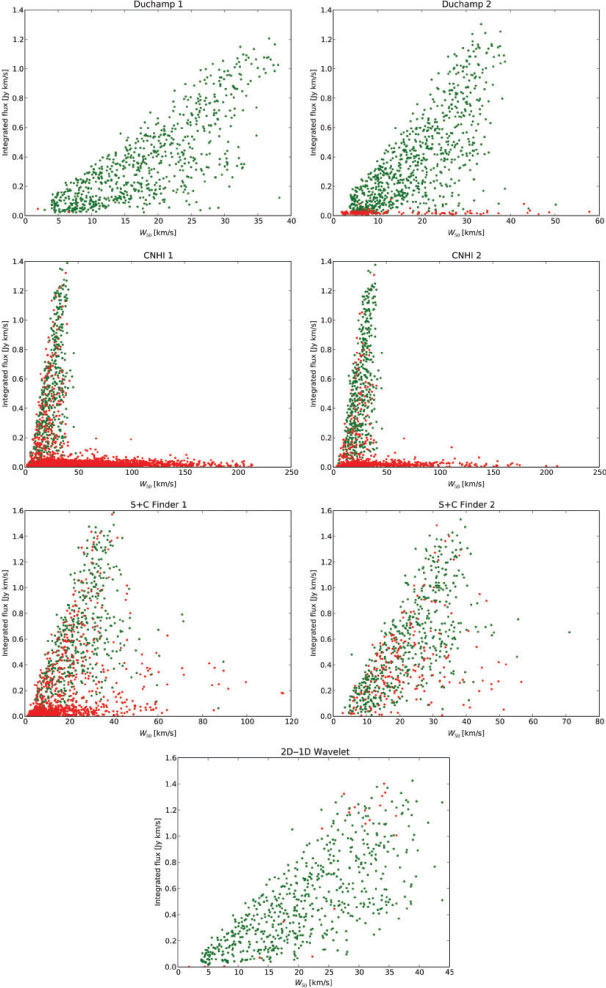
|
In the duchamp results for the point sources shown in the top panels of Figure 6 there are barely any false detections in the first run. In the second run, all false detections have low fluxes. A possibility that can improve the reliability is to apply a cut in integrated flux after the parametrisation of detections. In this example a cut a 0.05 Jy km s–1 would increase the reliability to ~100% while the number of missed real detections is still limited.
For the cnhi finder the difference between true and false detections is not so obvious. False detections are not clustered in a clearly defined parameter space, but rather mixed with real detections, making it more difficult to eliminate them after post-processing. There is however a very large bulge of detections with a low flux and broad line width.
The s+c finder has a large number of false detections in the first run, however a very large fraction can be eliminated by applying a cut in integrated flux. In the second run the number of false detections is much lower, however they are very well mixed with true detections and difficult to eliminate. Although not shown in the plot, particular for this source finder is that it also reports negative fluxes. These are by default all considered false detections. Assuming that the noise is symmetric, the reliability of positive detections can be determined based on the properties of the negative detections. This method is further explored and explained in Serra, Jurek & Flöer (2012).
The 2d–1d wavelet source finder is very reliable for point sources as shown before, with barely any false detections. The false detections are however difficult to eliminate as they are concentrated toward high fluxes and line widths. As mentioned this could be a consequence of the used test cube which has a very high source density. Especially in the case of strong sources the largest wavelet scales will merge sources, decreasing the number of detected objects and hence the completeness.
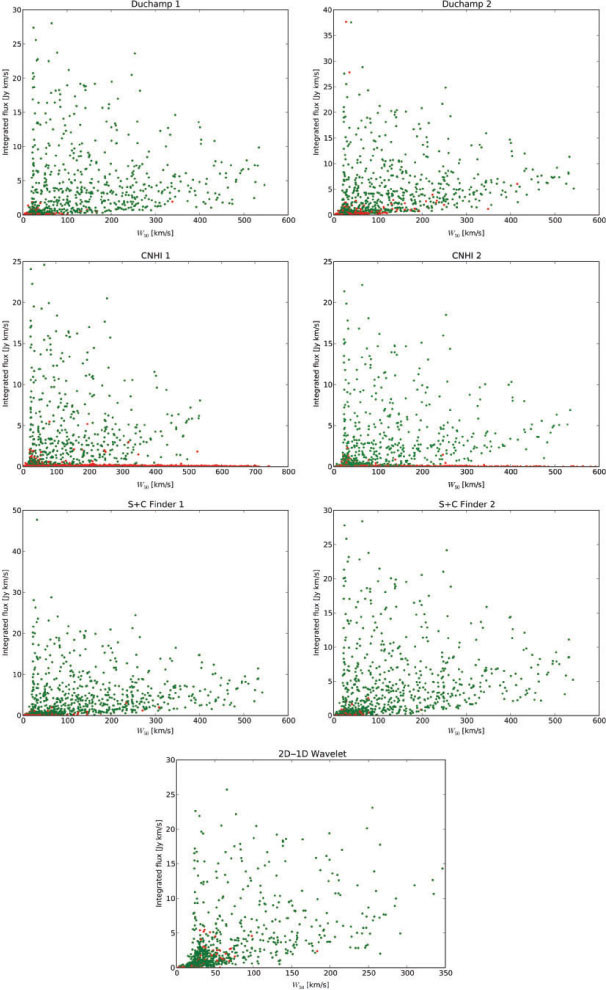
A very similar set of plots is given in Figure 7, where true and false detections of the model galaxies are plotted for all the source finders apart from gamma-finder. The behaviour of the different algorithms is very similar to before, where the false detections of duchamp tend to have a low integrated flux, although it is difficult to completely isolate them. The cnhi finder has a very large number of false detection with low flux and broad line-width, many of which can be rejected to refine the reliability. The performance of the s+c finder is very good when it comes to reliability as the number of false detections is relatively low. Also the reliability of the 2d–1d wavelet finder is very good, however the false detections are mixed with true detections.
|
The reliability of the source finders can be dramatically improved upon through simple cuts in parameter space. To be able to do this, it is crucial to properly parameterise the detections which has not been done sufficiently at this stage. Nevertheless, to illustrate the concept, we applied a cut on the detections at different integrated flux levels. In Figure 8 the results are shown, where completeness is plotted as function of reliability for the different source finders after applying cuts at different flux levels. For the point sources cuts have been applied at Fint = 0.0, 0.01, 0.02, 0.03, 0.04 and 0.05 Jy km s–1 while for the model galaxies at Fint = 0.0, 0.1, 0.2, 0.3, 0.4 and 0.5 Jy km s–1. The results move from high completeness and low reliabiliy when not applying a cut to low completeness and high realiability when applying the most extreme cut. Although the improvements in reliability vary amongst the different source finders, for each of them the raw reliability can be improved by tens of percent, while only losing a few percent in completeness. In the case of the second duchamp test on the point sources the reliability increases from 72% to 96%, while the completeness drops by only 0.6% from 83% to 82% at the fourth data point. On the model galaxies the most impressive result is achieved with the s+c finder where in the second run the reliability increases to above 95%, while still maintaining a completeness of almost 70%.

|
6 Conclusions
In this paper we have compared the performance of five potential ASKAP Hi source finders. The tested source finders are 1) duchamp, 2) gamma-finder, 3) the cnhi source finder, 4) the 2d–1d wavelet reconstruction source finder and 5) the s+c finder, a source finder based on sigma clipping of smoothed versions of the original data cube. The source finders have been applied to two data cubes with model sources, the first containing point sources with a relatively narrow Gaussian line profile and the second containing extended galaxies with inclinations and rotation curves.
We have to stress that apart from gamma-finder the tested source finders are not final products but are still under active development. In this paper we want to present the current status of the different source finders, however there is significant room for improvement as is also discussed in other papers in this issue describing some of the tested source finders individually.
The testing of different source finding algorithms on different data cubes has proven that it is very difficult to find a good source finder which is reliable for many types of objects. Source finders perform very differently depending on the type of object that is detected.
An important feature of a source finder is its reliability, which has not yet been fully explored. Although a number for the raw reliability can be given, in many cases the false detections are clustered within a certain range of flux and line width. We are confident that a large fraction of the false detections can be rejected through simple cuts in parameter space as has been demonstrated in the discussion, however to be able to do this properly all detections have to be parameterised accurately which has not been done yet.
For the current source finders and datasets, we find that for point sources 50% completeness can be achieved at an integrated signal-to-noise ratio of ~4–5 sigma, and 100% completeness can be achieved around an integrated signal-to-noise ratio of ~10. For the extended sources the completeness estimates are very similar: for the best results 50% completeness is achieved at an integrated signal-to-noise ratio of ~4–6 and 100% completeness is achieved at an integrated signal-to-noise ratio of ~10.
It is interesting to see that the different source finders achieve a different performance, depending on the type of object. Currently none of the source finders excels at being able to achieve the best result in the full parameter space when looking at integrated flux and line width. Nevertheless we have pointed out the strong and weak points of the different source finders, which provides input for future development and testing.
For the tested parameters, currently duchamp gives the best results on point sources, while the s+c finder gives the best result for extended objects when looking at the completeness. Due to the different smoothing levels that have been applied in the s+c finder, this algorithm is best capable of matching the true shape of an object. As the s+c finder concept is simple yet powerful, we recommend that the other source finders improve their performance by incorporating smoothing on multiple scales.
Currently all the tested source finders perform reasonably well, however there is significant room for improvement to meet our goals. All of the source finders have a certain area in parameter space where they perform best and we will combine the algorithms of different source finders to optimise the result.
Duffy et al. (A. R. Duffy 2011, in preparation) give predictions of the number of objects that will be detected with WALLABY and DINGO. They predict that at an angular resolution of 30″, 14% of the WALLABY sources will be unresolved and the bulk of the remainder will be marginally resolved, while for DINGO 93.3% of the sources will be unresolved. This means that many of the unresolved sources in DINGO will have very different profiles to the ones tested in this paper. At an angular resolution of 10″ these numbers change dramatically, as for WALLABY none of the sources will be point sources as all sources will be larger than one beam, and for DINGO 7.4% of the objects will be smaller than one beam.
Although the two cubes that have been used for testing cover a large area in parameter space, they do not sample the full signal-to-noise ratio range properly. We have started efforts to test the source finders on models covering a large range of parameters, keeping integrated signal-to-noise values constant. These tests should give accurate estimates of how many sources can be detected by WALLABY and DINGO.
We have a fairly good understanding of the different source finders on simulated objects as presented in this paper. The cubes that have been tested are ideal cubes in the sense that the noise is Gaussian and does not have any systematic artefacts caused by continuum sources, solar ripples, phase errors, radio frequency interference, etc. These contributions have not been taken into account but will have a very significant effect on the performance of source finders, especially in terms of reliability. The simulated model sources are perfectly symmetric sources without any weird or unexpected shapes or extended tails. To have a better understanding of the performance of the source finders, the next step will be to test the source finders on a cube containing data from real galaxies as they occur in the Universe.
References
Boyce, P., 2003, MSc Dissertation, University of CardiffDeboer, D. R. et al., 2009, IEEEP, 97, 1507
Dewdney, P. E., Hall, P. J., Schilizzi, R. T. and Lazio, T. J. L., 2009, IEEEP, 97, 1482
Driver, S. P. et al., 1999, A&G, 50, 12
Flöer, L. and Winkel, B., 2012, PASA, 29, 244
| Crossref | GoogleScholarGoogle Scholar |
Haynes, M. P. et al., 2011, AJ, 142, 170
Hibbard, J. E., van Gorkom, J. H., Rupen, M. P. and Schiminovich, D., 2001, ASPC, 240, 657
Johnston, S. et al., 2008, ExA, 22, 151
Jonas, J. L., 2009, IEEEP, 97, 1522
Jones, A. J., Evans, D., Margetts, S. & Durrant, P. J., 2002, in Heuristic and Optimization for Knowledge Discovery, ed. H. A. Abbass, C. S. Newton & R. Sarker (Hershey: Idea Group Publishing), 142
Jurek, R., 2012, PASA, 29, 251
| Crossref | GoogleScholarGoogle Scholar |
Koribalski, B. S. & Staveley-Smith, L., 2009, ASKAP Survey Science Proposal
Koribalski, B. S. et al., 2004, AJ, 128, 16
| 1:CAS:528:DC%2BD2cXmsVagt7Y%3D&md5=7e2f111351d39252b92d0fdc54b66155CAS |
Meyer, M. J. et al., 2004, MNRAS, 350, 1195
| Crossref | GoogleScholarGoogle Scholar | 1:CAS:528:DC%2BD2cXls1Sjurc%3D&md5=a45ea5e988dc074b2b07256ef6e8123aCAS |
Meyer, M., 2009, in Panoramic Radio Astronomy: Wide-field 1–2 GHz Research on Galaxy Evolution, ed. G. Heald & P. Serra, Proceedings of Science, PoS(PRA2009)015
Minchin, R. F. et al., 2003, MNRAS, 346, 787
| Crossref | GoogleScholarGoogle Scholar | 1:CAS:528:DC%2BD2cXksVeluw%3D%3D&md5=59d741392ccfa81c0dc56bead90a29d7CAS |
Putman, M. E. et al., 2002, AJ, 123, 873
Serra, P., et al., 2011, MNRAS, submitted
Serra, P., Jurek, R. and Flöer, L., 2012, PASA, 29, 296
| Crossref | GoogleScholarGoogle Scholar |
Springob, C. M. et al., 2005, ApJS, 160, 149
| Crossref | GoogleScholarGoogle Scholar | 1:CAS:528:DC%2BD2MXhtVOltLrM&md5=cad0e3887dc85b70c3c31524f2de3d8fCAS |
Starck, J. L., Fadili, J. M., Digel, S., Zhang, B. and Chiang, J., 2009, A&A, 504, 641
| 1:CAS:528:DC%2BD1MXhtlWltb%2FK&md5=2fe64a2a0de6b31befa1832bb5853536CAS |
Stefansson, A., Koncar, N. and Jones, A. J., 1997, Neural Computing and Applications, 5, 131
| Crossref | GoogleScholarGoogle Scholar |
Verheijen, M. A. W., Oosterloo, T. A., van Cappellen, W. A., Bakker, L., Ivashina, M. V. and van der Hulst, J. M., 2008, AIPC, 1035, 265
| 1:CAS:528:DC%2BD1cXpslSjt7s%3D&md5=7c0ea63b8a7ed621fd049d877fc5e414CAS |
Westmeier, T., Popping, A. and Serra, P., 2012, PASA, 29, 276
| Crossref | GoogleScholarGoogle Scholar |
Whiting, M. T., 2011, MNRAS, arXiv1201.2710
1 duchamp website: