

The Fine-Tuning of the Universe for Intelligent Life
L. A. BarnesInstitute for Astronomy, ETH Zurich, Switzerland, and Sydney Institute for Astronomy, School of Physics, University of Sydney, Australia. Email: L.Barnes@physics.usyd.edu.au
Publications of the Astronomical Society of Australia 29(4) 529-564 https://doi.org/10.1071/AS12015
Submitted: 6 February 2012 Accepted: 24 April 2012 Published: 7 June 2012
Journal Compilation © Astronomical Society of Australia 2012
Abstract
The fine-tuning of the universe for intelligent life has received a great deal of attention in recent years, both in the philosophical and scientific literature. The claim is that in the space of possible physical laws, parameters and initial conditions, the set that permits the evolution of intelligent life is very small. I present here a review of the scientific literature, outlining cases of fine-tuning in the classic works of Carter, Carr and Rees, and Barrow and Tipler, as well as more recent work. To sharpen the discussion, the role of the antagonist will be played by Victor Stenger’s recent book The Fallacy of Fine-Tuning: Why the Universe is Not Designed for Us. Stenger claims that all known fine-tuning cases can be explained without the need for a multiverse. Many of Stenger’s claims will be found to be highly problematic. We will touch on such issues as the logical necessity of the laws of nature; objectivity, invariance and symmetry; theoretical physics and possible universes; entropy in cosmology; cosmic inflation and initial conditions; galaxy formation; the cosmological constant; stars and their formation; the properties of elementary particles and their effect on chemistry and the macroscopic world; the origin of mass; grand unified theories; and the dimensionality of space and time. I also provide an assessment of the multiverse, noting the significant challenges that it must face. I do not attempt to defend any conclusion based on the fine-tuning of the universe for intelligent life. This paper can be viewed as a critique of Stenger’s book, or read independently.
Keywords: cosmology: theory — history and philosophy of astronomy
1 Introduction
The fine-tuning of the universe for intelligent life has received much attention in recent times. Beginning with the classic papers of Carter (1974) and Carr & Rees (1979), and the extensive discussion of Barrow & Tipler (1986), a number of authors have noticed that very small changes in the laws, parameters and initial conditions of physics would result in a universe unable to evolve and support intelligent life.
We begin by defining our terms. We will refer to the laws of nature, initial conditions and physical constants of a particular universe as its physics for short. Conversely, we define a ‘universe’ be a connected region of spacetime over which physics is effectively constant1. The claim that the universe is fine-tuned can be formulated as:
FT: In the set of possible physics, the subset that permit the evolution of life is very small.
FT can be understood as a counterfactual claim, that is, a claim about what would have been. Such claims are not uncommon in everyday life. For example, we can formulate the claim that Roger Federer would almost certainly defeat me in a game of tennis as: ‘in the set of possible games of tennis between myself and Roger Federer, the set in which I win is extremely small’. This claim is undoubtedly true, even though none of the infinitely-many possible games has been played.
Our formulation of FT, however, is in obvious need of refinement. What determines the set of possible physics? Where exactly do we draw the line between ‘universes’? How is ‘smallness’ being measured? Are we considering only cases where the evolution of life is physically impossible or just extremely improbable? What is life? We will press on with the our formulation of FT as it stands, pausing to note its inadequacies when appropriate. As it stands, FT is precise enough to distinguish itself from a number of other claims for which it is often mistaken. FT is not the claim that this universe is optimal for life, that it contains the maximum amount of life per unit volume or per baryon, that carbon-based life is the only possible type of life, or that the only kinds of universes that support life are minor variations on this universe. These claims, true or false, are simply beside the point.
The reason why FT is an interesting claim is that it makes the existence of life in this universe appear to be something remarkable, something in need of explanation. The intuition here is that, if ours were the only universe, and if the causes that established the physics of our universe were indifferent to whether it would evolve life, then the chances of hitting upon a life-permitting universe are very small. As Leslie (1989, p. 121) notes, ‘[a] chief reason for thinking that something stands in special need of explanation is that we actually glimpse some tidy way in which it might be explained’. Consider the following tidy explanations:
-
This universe is one of a large number of variegated universes, produced by physical processes that randomly scan through (a subset of) the set of possible physics. Eventually (or somewhere), a life-permitting universe will be created. Only such universes can be observed, since only such universes contain observers.
-
There exists a transcendent, personal creator of the universe. This entity desires to create a universe in which other minds will be able to form. Thus, the entity chooses from the set of possibilities a universe which is foreseen to evolve intelligent life2.
These scenarios are neither mutually exclusive nor exhaustive, but if either or both were true then we would have a tidy explanation of why our universe, against the odds, supports the evolution of life.
Our discussion of the multiverse will touch on the so-called anthropic principle, which we will formulate as follows:
AP: If observers observe anything, they will observe conditions that permit the existence of observers.
Tautological? Yes! The anthropic principle is best thought of as a selection effect. Selection effects occur whenever we observe a non-random sample of an underlying population. Such effects are well known to astronomers. An example is Malmquist bias — in any survey of the distant universe, we will only observe objects that are bright enough to be detected by our telescope. This statement is tautological, but is nevertheless non-trivial. The penalty of ignoring Malmquist bias is a plague of spurious correlations. For example, it will seem that distant galaxies are on average intrinsically brighter than nearby ones.
A selection bias alone cannot explain anything. Consider quasars: when first discovered, they were thought to be a strange new kind of star in our galaxy. Schmidt (1963) measured their redshift, showing that they were more than a million times further away than previously thought. It follows that they must be incredibly bright. How are quasars so luminous? The (best) answer is: because quasars are powered by gravitational energy released by matter falling into a super-massive black hole (Zel'dovich 1964; Lynden-Bell 1969). The answer is not: because otherwise we wouldn’t see them. Noting that if we observe any object in the very distant universe then it must be very bright does not explain why we observe any distant objects at all. Similarly, AP cannot explain why life and its necessary conditions exist at all.
In anticipation of future sections, Table 1 defines some relevant physical quantities.

|
2 Cautionary Tales
There are a few fallacies to keep in mind as we consider cases of fine-tuning.
The Cheap-Binoculars Fallacy: ‘Don’t waste money buying expensive binoculars. Simply stand closer to the object you wish to view’3. We can make any point (or outcome) in possibility space seem more likely by zooming-in on its neighbourhood. Having identified the life-permitting region of parameter space, we can make it look big by deftly choosing the limits of the plot. We could also distort parameter space using, for example, logarithmic axes.
A good example of this fallacy is quantifying the fine-tuning of a parameter relative to its value in our universe, rather than the totality of possibility space. If a dart lands 3 mm from the centre of a dartboard, is it obviously fallacious to say that because the dart could have landed twice as far away and still scored a bullseye, therefore the throw is only fine-tuned to a factor of two and there is ‘plenty of room’ inside the bullseye. The correct comparison is between the area of the bullseye and the area in which the dart could land. Similarly, comparing the life-permitting range to the value of the parameter in our universe necessarily produces a bias toward underestimating fine-tuning, since we know that our universe is in the life-permitting range.
The Flippant Funambulist Fallacy: ‘Tightrope-walking is easy!’, the man says, ‘just look at all the places you could stand and not fall to your death!’. This is nonsense, of course: a tightrope walker must overbalance in a very specific direction if her path is to be life-permitting. The freedom to wander is tightly constrained. When identifying the life-permitting region of parameter space, the shape of the region is irrelevant. An elongated life-friendly region is just as fine-tuned as a compact region of the same area. The fact that we can change the setting on one cosmic dial, so long as we very carefully change another at the same time, does not necessarily mean that FT is false.
The Sequential Juggler Fallacy: ‘Juggling is easy!’, the man says, ‘you can throw and catch a ball. So just juggle all five, one at a time’. Juggling five balls one-at-a-time isn’t really juggling. For a universe to be life-permitting, it must satisfy a number of constraints simultaneously. For example, a universe with the right physical laws for complex organic molecules, but which recollapses before it is cool enough to permit neutral atoms will not form life. One cannot refute FT by considering life-permitting criteria one-at-a-time and noting that each can be satisfied in a wide region of parameter space. In set-theoretic terms, we are interested in the intersection of the life-permitting regions, not the union.
The Cane Toad Solution: In 1935, the Bureau of Sugar Experiment Stations was worried by the effect of the native cane beetle on Australian sugar cane crops. They introduced 102 cane toads, imported from Hawaii, into parts of Northern Queensland in the hope that they would eat the beetles. And thus the problem was solved forever, except for the 200 million cane toads that now call eastern Australia home, eating smaller native animals, and secreting a poison that kills any larger animal that preys on them. A cane toad solution, then, is one that doesn’t consider whether the end result is worse than the problem itself. When presented with a proposed fine-tuning explainer, we must ask whether the solution is more fine-tuned than the problem.
3 Stenger’s Case
We will sharpen the presentation of cases of fine-tuning by responding to the claims of Victor Stenger. Stenger is a particle physicist whose latest book, ‘The Fallacy of Fine-Tuning: Why the Universe is Not Designed for Us’4, makes the following bold claim:
‘The most commonly cited examples of apparent fine-tuning can be readily explained by the application of a little well-established physics and cosmology. …Some form of life would have occurred in most universes that could be described by the same physical models as ours, with parameters whose ranges varied over ranges consistent with those models. And I will show why we can expect to be able to describe any uncreated universe with the same models and laws with at most slight, accidental variations. Plausible natural explanations can be found for those parameters that are most crucial for life. …My case against fine-tuning will not rely on speculations beyond well-established physics nor on the existence of multiple universes.’ (Foft 22, 24)
Let’s be clear on the task that Stenger has set for himself. There are a great many scientists, of varying religious persuasions, who accept that the universe is fine-tuned for life, e.g. Barrow, Carr, Carter, Davies, Dawkins, Deutsch, Ellis, Greene, Guth, Harrison, Hawking, Linde, Page, Penrose, Polkinghorne, Rees, Sandage, Smolin, Susskind, Tegmark, Tipler, Vilenkin, Weinberg, Wheeler, Wilczek5. They differ, of course, on what conclusion we should draw from this fact. Stenger, on the other hand, claims that the universe is not fine-tuned.
4 Cases of Fine-Tuning
What is the evidence that FT is true? We would like to have meticulously examined every possible universe and determined whether any form of life evolves. Sadly, this is currently beyond our abilities. Instead, we rely on simplified models and more general arguments to step out into possible-physics-space. If the set of life-permitting universes is small amongst the universes that we have been able to explore, then we can reasonably infer that it is unlikely that the trend will be miraculously reversed just beyond the horizon of our knowledge.
4.1 The Laws of Nature
Are the laws of nature themselves fine-tuned? Foft defends the ambitious claim that the laws of nature could not have been different because they can be derived from the requirement that they be Point-of-View Invariant (hereafter, PoVI). He says:
‘…[In previous sections] we have derived all of classical physics, including classical mechanics, Newton’s law of gravity, and Maxwell’s equations of electromagnetism, from just one simple principle: the models of physics cannot depend on the point of view of the observer. We have also seen that special and general relativity follow from the same principle, although Einstein’s specific model for general relativity depends on one or two additional assumptions. I have offered a glimpse at how quantum mechanics also arises from the same principle, although again a few other assumptions, such as the probability interpretation of the state vector, must be added. …[The laws of nature] will be the same in any universe where no special point of view is present.’ (Foft 88, 91)
4.1.1 Invariance, Covariance and Symmetry
We can formulate Stenger’s argument for this conclusion as follows:
-
LN1. If our formulation of the laws of nature is to be objective, it must be PoVI.
-
LN2. Invariance implies conserved quantities (Noether’s theorem).
-
LN3. Thus, ‘when our models do not depend on a particular point or direction in space or a particular moment in time, then those models must necessarily [emphasis original] contain the quantities linear momentum, angular momentum, and energy, all of which are conserved. Physicists have no choice in the matter, or else their models will be subjective, that is, will give uselessly different results for every different point of view. And so the conservation principles are not laws built into the universe or handed down by deity to govern the behavior of matter. They are principles governing the behavior of physicists.’ (Foft 82)
This argument commits the fallacy of equivocation — the term ‘invariant’ has changed its meaning between LN1 and LN2. The difference is decisive but rather subtle, owing to the different contexts in which the term can be used. We will tease the two meanings apart by defining covariance and symmetry, considering a number of test cases.
Galileo’s Ship: We can see where Stenger’s argument has gone wrong with a simple example, before discussing technicalities in later sections. Consider this delightful passage from Galileo regarding the brand of relativity that bears his name:
‘Shut yourself up with some friend in the main cabin below decks on some large ship, and have with you there some flies, butterflies, and other small flying animals. Have a large bowl of water with some fish in it; hang up a bottle that empties drop by drop into a wide vessel beneath it. With the ship standing still, observe carefully how the little animals fly with equal speed to all sides of the cabin. The fish swim indifferently in all directions; the drops fall into the vessel beneath; and, in throwing something to your friend, you need throw it no more strongly in one direction than another, the distances being equal; jumping with your feet together, you pass equal spaces in every direction. When you have observed all these things carefully, …have the ship proceed with any speed you like, so long as the motion is uniform and not fluctuating this way and that. You will discover not the least change in all the effects named, nor could you tell from any of them whether the ship was moving or standing still.’ (Quoted in Healey (2007, chapter 6).).
Note carefully what Galileo is not saying. He is not saying that the situation can be viewed from a variety of different viewpoints and it looks the same. He is not saying that we can describe flight-paths of the butterflies using a coordinate system with any origin, orientation or velocity relative to the ship.
Rather, Galileo’s observation is much more remarkable. He is stating that the two situations, the stationary ship and moving ship, which are externally distinct are nevertheless internally indistinguishable. The two situations cannot be distinguished by means of measurements confined to each situation (Healey 2007, Chapter 6). These are not different descriptions of the same situation, but rather different situations with the same internal properties.
The reason why Galilean relativity is so shocking and counterintuitive is that there is no a priori reason to expect distinct situations to be indistinguishable. If you and your friend attempt to describe the butterfly in the stationary ship and end up with ‘uselessly different results’, then at least one of you has messed up your sums. If your friend tells you his point-of-view, you should be able to perform a mathematical transformation on your model and reproduce his model. None of this will tell you how the butterflies will fly when the ship is speeding on the open ocean. An Aristotelian butterfly would presumably be plastered against the aft wall of the cabin. It would not be heard to cry: ‘Oh, the subjectivity of it all!’
Galilean invariance, and symmetries in general, have nothing whatsoever to do with point-of-view invariance. A universe in which Galilean relativity did not hold would not wallow in subjectivity. It would be an objective, observable fact that the butterflies would fly differently in a speeding ship. This is Stenger’s confusion: PoVI does not imply symmetry.
Lagrangian Dynamics: We can see this same point in a more formal context. Lagrangian dynamics is a framework for physical theories that, while originally developed as a powerful approach to Newtonian dynamics, underlies much of modern physics. The method revolves around a mathematical function  called the Lagrangian, where t is time, the variables qi parameterise the degrees of freedom (the ‘coordinates’), and
  . For a system described by L, the equations of motion can be derived from L via the Euler–Lagrange equation.
One of the features of the Lagrangian formalism is that it is covariant. Suppose that we want to use different coordinates for our system, say si, that are expressed as functions of the old coordinates qi and t. We can express the Lagrangian L in terms of t, si and  by substituting the new coordinates for the old ones. Crucially, the form of the Euler–Lagrange equation does not change — just replace q with s. In other words, it does not matter what coordinates we use. The equations take the same form in any coordinate system, and are thus said to be covariant. Note that this is true of any Lagrangian, and any (sufficiently smooth) coordinate transformation si(t, qj). Objectivity (and PoVI) are guaranteed.
Now, consider a specific Lagrangian L that has the following special property — there exists a continuous family of coordinate transformations that leave L unchanged. Such a transformation is called a symmetry (or isometry) of the Lagrangian. The simplest case is where a particular coordinate does not appear in the expression for L. Noether’s theorem tells us that, for each continuous symmetry, there will be a conserved quantity. For example, if time does not appear explicitly in the Lagrangian, then energy will be conserved.
Note carefully the difference between covariance and symmetry. Both could justifiably be called ‘coordinate invariance’ but they are not the same thing. Covariance is a property of the entire Lagrangian formalism. A symmetry is a property of a particular Lagrangian L. Covariance holds with respect to all (sufficiently smooth) coordinate transformations. A symmetry is linked to a particular coordinate transformation. Covariance gives us no information whatsoever about which Lagrangian best describes a given physical scenario. Symmetries provide strong constraints on the which Lagrangians are consistent with empirical data. Covariance is a mathematical fact about our formalism. Symmetries can be confirmed or falsified by experiment.
Lorentz Invariance: Let’s look more closely at some specific cases. Stenger applies his general PoVI argument to Einstein’s special theory of relativity:
‘Special relativity similarly results from the principle that the models of physics must be the same for two observers moving at a constant velocity with respect to one another. …Physicists are forced to make their models Lorentz invariant so they do not depend on the particular point of view of one reference frame moving with respect to another.’
This claim is false. Physicists are perfectly free to postulate theories which are not Lorentz invariant, and a great deal of experimental and theoretical effort has been expended to this end. The compilation of Kostelecký & Russell (2011) cites 127 papers that investigate Lorentz violation. Pospelov & Romalis (2004) give an excellent overview of this industry, giving an example of a Lorentz-violating Lagrangian:

where the fields bμ, kμ and Hμν are external vector and antisymmetric tensor backgrounds that introduce a preferred frame and therefore break Lorentz invariance; all other symbols have their usual meanings (e.g. Nagashima 2010). A wide array of laboratory, astrophysical and cosmological tests place impressively tight bounds on these fields. At the moment, the violation of Lorentz invariance is just a theoretical possibility. But that’s the point.
Ironically, the best cure for a conflation of ‘frame-dependent’ with ‘subjective’ is special relativity. The length of a rigid rod depends on the reference frame of the observer: if it is 2 metres long it its own rest frame, it will be 1 metre long in the frame of an observer passing at 87% of the speed of light6. It does not follow that the length of the rod is ‘subjective’, in the sense that the length of the rod is just the personal opinion of a given observer, or in the sense that these two different answers are ‘uselessly different’. It is an objective fact that the length of the rod is frame-dependent. Physics is perfectly capable of studying frame-dependent quantities, like the length of a rod, and frame-dependent laws, such as the Lagrangian in Equation 1.
General Relativity: We turn now to Stenger’s discussion of gravity.
‘Ask yourself this: If the gravitational force can be transformed away by going to a different reference frame, how can it be ‘real’? It can’t. We see that the gravitational force is an artifact, a ‘fictitious’ force just like the centrifugal and Coriolis forces. …[If there were no gravity] then there would be no universe. …[P]hysicists have to put gravity into any model of the universe that contains separate masses. A universe with separated masses and no gravity would violate point-of-view invariance. …In general relativity, the gravitational force is treated as a fictitious force like the centrifugal force, introduced into models to preserve invariance between reference frames accelerating with respect to one another.’
These claims are mistaken. The existence of gravity is not implied by the existence of the universe, separate masses or accelerating frames.
Stenger’s view may be rooted in the rather persistent myth that special relativity cannot handle accelerating objects or frames, and so general relativity (and thus gravity) is required. The best remedy to this view to sit down with the excellent textbook of Hartle (2003) and don’t get up until you’ve finished Chapter 5’s ‘systematic way of extracting the predictions for observers who are not associated with global inertial frames …in the context of special relativity’. Special relativity is perfectly able to preserve invariance between reference frames accelerating with respect to one another. Physicists clearly don’t have to put gravity into any model of the universe that contains separate masses.
We can see this another way. None of the invariant/covariant properties of general relativity depend on the value of Newton’s constant G. In particular, we can set G = 0. In such a universe, the geometry of spacetime would not be coupled to its matter-energy content, and Einstein’s equation would read Rμν = 0. With no source term, local Lorentz invariance holds globally, giving the Minkowski metric of special relativity. Neither logical necessity nor PoVI demands the coupling of spacetime geometry to mass-energy. This G = 0 universe is a counterexample to Stenger’s assertion that no gravity means no universe.
What of Stenger’s claim that general relativity is merely a fictitious force, to be derived from PoVI and ‘one or two additional assumptions’? Interpreting PoVI as what Einstein called general covariance, PoVI tells us almost nothing. General relativity is not the only covariant theory of spacetime (Norton 1995). As Misner, Thorne & Wheeler (1973, p. 302) note: ‘Any physical theory originally written in a special coordinate system can be recast in geometric, coordinate-free language. Newtonian theory is a good example, with its equivalent geometric and standard formulations. Hence, as a sieve for separating viable theories from nonviable theories, the principle of general covariance is useless.’ Similarly, Carroll (2003) tells us that the principle ‘Laws of physics should be expressed (or at least be expressible) in generally covariant form’ is ‘vacuous’. We can now identify the ‘additional assumptions’ that Stenger needs to derive general relativity. Given general covariance (or PoVI), the additional assumptions constitute the entire empirical content of the theory.
Finally, general relativity provides a perfect counterexample to Stenger’s conflation of covariance with symmetry. Einstein’s GR field equation is covariant — it takes the same form in any coordinate system, and applying a coordinate transformation to a particular solution of the GR equation yields another solution, both representing the same physical scenario. Thus, any solution of the GR equation is covariant, or PoVI. But it does not follow that a particular solution will exhibit any symmetries. There may be no conserved quantities at all. As Hartle (2003, pp. 176, 342) explains:
‘Conserved quantities …cannot be expected in a general spacetime that has no special symmetries …The conserved energy and angular momentum of particle orbits in the Schwarzschild geometry7 followed directly from its time displacement and rotational symmetries. …But general relativity does not assume a fixed spacetime geometry. It is a theory of spacetime geometry, and there are no symmetries that characterize all spacetimes.’
The Standard Model of Particle Physics and Gauge Invariance: We turn now to particle physics, and particularly the gauge principle. Interpreting gauge invariance as ‘just a fancy technical term for point-of-view invariance’, Stenger says:
‘If [the phase of the wavefunction] is allowed to vary from point to point in space-time, Schrödinger’s time-dependent equation …is not gauge invariant. However, if you insert a four-vector field into the equation and ask what that field has to be to make everything nice and gauge invariant, that field is precisely the four-vector potential that leads to Maxwell’s equations of electromagnetism! That is, the electromagnetic force turns out to be a fictitious force, like gravity, introduced to preserve the point-of-view invariance of the system. …Much of the standard model of elementary particles also follows from the principle of gauge invariance.’ (Foft 86–88)
Remember the point that Stenger is trying to make: the laws of nature are the same in any universe which is point-of-view invariant.
Stenger’s discussion glosses over the major conceptual leap from global to local gauge invariance. Most discussions of the gauge principle are rather cautious at this point. Yang, who along with Mills first used the gauge principle as a postulate in a physical theory, commented that ‘We did not know how to make the theory fit experiment. It was our judgement, however, that the beauty of the idea alone merited attention’. Kaku (1993, p. 11), who provides this quote, says of the argument for local gauge invariance:
‘If the predictions of gauge theory disagreed with the experimental data, then one would have to abandon them, no matter how elegant or aesthetically satisfying they were. Gauge theorists realized that the ultimate judge of any theory was experiment.’
Similarly, Griffiths (2008) ‘knows of no compelling physical argument for insisting that global invariance should hold locally’ [emphasis original]. Aitchison & Hey (2002) says that this line of thought is ‘not compelling motivation’ for the step from global to local gauge invariance, and along with Pokorski (2000), who describes the argument as aesthetic, ultimately appeals to the empirical success of the principle for justification. Needless to say, these are not the views of physicists demanding that all possible universes must obey a certain principle8. We cannot deduce gauge invariance from PoVI.
Even with gauge invariance, we are still a long way from the standard model of particle physics. A gauge theory needs a symmetry group. Electromagnetism is based on U(1), the weak force SU(2), the strong force SU(3), and there are grand unified theories based on SU(5), SO(10), E8 and more. These are just the theories with a chance of describing our universe. From a theoretical point of view, there are any number of possible symmetries, e.g. SU(N) and SO(N) for any integer N (Schellekens 2008). The gauge group of the standard model, SU(3) × SU(2) × U(1), is far from unique.
Conclusion: We can now see the flaw in Stenger’s argument. Premise LN1 should read: If our formulation of the laws of nature is to be objective, then it must be covariant. Premise LN2 should read: symmetries imply conserved quantities. Since ‘covariant’ and ‘symmetric’ are not synonymous, it follows that the conclusion of the argument is unproven, and we would argue that it is false. The conservation principles of this universe are not merely principles governing our formulation of the laws of nature. Neother’s theorems do not allow us to pull physically significant conclusions out of a mathematical hat. If you want to know whether a certain symmetry holds in nature, you need a laboratory or a telescope, not a blackboard. Symmetries tell us something about the physical universe.
4.1.2 Is Symmetry Enough?
Suppose that Stenger were correct regarding symmetries, that any objective description of the universe must incorporate them. One of the features of the universe as we currently understand it is that it is not perfectly symmetric. Indeed, intelligent life requires a measure of asymmetry. For example, the perfect homogeneity and isotropy of the Robertson–Walker spacetime precludes the possibility of any form of complexity, including life. Sakharov (1967) showed that for the universe to contain sufficient amounts of ordinary baryonic matter, interactions in the early universe must violate baryon number conservation, charge-symmetry and charge-parity-symmetry, and must spend some time out of thermal equilibrium. Supersymmetry, too, must be a broken symmetry in any life-permitting universe, since the bosonic partner of the electron (the selectron) would make chemistry impossible (see the discussion in Susskind 2005, p. 250). As Pierre Curie has said, it is asymmetry that creates a phenomena.
One of the most important concepts in modern physics is spontaneous symmetry breaking (SSB). The power of SSB is that it allows us
‘…to understand how the conclusions of the Noether theorem can be evaded and how a symmetry of the dynamics cannot be realized as a mapping of the physical configurations of the system.’ (Strocchi 2007, p. 3)
SSB allows the laws of nature to retain their symmetry and yet have asymmetric solutions. Even if the symmetries of the laws of nature were logically necessary, it would still be an open question as to precisely which symmetries were broken in our universe and which were unbroken.
4.1.3 Changing the Laws of Nature
What if the laws of nature were different? Stenger says:
‘…what about a universe with a different set of ‘laws’? There is not much we can say about such a universe, nor do we need to. Not knowing what any of their parameters are, no one can claim that they are fine-tuned.’ (Foft 69)
In reply, fine-tuning isn’t about what the parameters and laws are in a particular universe. Given some other set of laws, we ask: if a universe were chosen at random from the set of universes with those laws, what is the probability that it would support intelligent life? If that probability is robustly small, then we conclude that that region of possible-physics-space contributes negligibly to the total life-permitting subset. It is easy to find examples of such claims.
-
A universe governed by Maxwell’s Laws ‘all the way down’ (i.e. with no quantum regime at small scales) would not have stable atoms — electrons radiate their kinetic energy and spiral rapidly into the nucleus — and hence no chemistry (Barrow & Tipler 1986, p. 303). We don’t need to know what the parameters are to know that life in such a universe is plausibly impossible.
-
If electrons were bosons, rather than fermions, then they would not obey the Pauli exclusion principle. There would be no chemistry.
-
If gravity were repulsive rather than attractive, then matter wouldn’t clump into complex structures. Remember: your density, thank gravity, is 1030 times greater than the average density of the universe.
-
If the strong force were a long rather than short-range force, then there would be no atoms. Any structures that formed would be uniform, spherical, undifferentiated lumps, of arbitrary size and incapable of complexity.
-
If, in electromagnetism, like charges attracted and opposites repelled, then there would be no atoms. As above, we would just have undifferentiated lumps of matter.
-
The electromagnetic force allows matter to cool into galaxies, stars, and planets. Without such interactions, all matter would be like dark matter, which can only form into large, diffuse, roughly spherical haloes of matter whose only internal structure consists of smaller, diffuse, roughly spherical subhaloes.
We should be cautious, however. Whatever the problems of defining the possible range of a given parameter, we are in a significantly more nebulous realm when we consider the set of all possible physical laws. It is not clear how such a fine-tuning case could be formalised, whatever its intuitive appeal.
4.2 The Wedge
Moving from the laws of nature to the parameters those laws, Stenger makes the following general argument against supposed examples of fine-tuning:
‘[T]he examples of fine-tuning given in the theist literature …vary one parameter while holding all the rest constant. This is both dubious and scientifically shoddy. As we shall see in several specific cases, changing one or more other parameters can often compensate for the one that is changed.’ (Foft 70)
To illustrate this point, Stenger introduces ‘the wedge’. I have produced my own version in Figure 1. Here, x and y are two physical parameters that can vary from zero to xmax and ymax, where we can allow these values to approach infinity if so desired. The point (x0, y0) represents the values of x and y in our universe. The life-permitting range is the shaded wedge. Stenger’s point is that varying only one parameter at a time only explores that part of parameter space which is vertically or horizontally adjacent to (x0, y0), thus missing most of parameter space. The probability of a life-permitting universe, assuming that the probability distribution is uniform in (x, y) — which, as Stenger notes, is ‘the best we can do’ (Foft 72) — is the ratio of the area inside the wedge to the area inside the dashed box.
|
4.2.1 The Wedge is a Straw Man
In response, fine-tuning relies on a number of independent life-permitting criteria. Fail any of these criteria, and life becomes dramatically less likely, if not impossible. When parameter space is explored in the scientific literature, it rarely (if ever) looks like the wedge. We instead see many intersecting wedges. Here are two examples.
Barr & Khan (2007) explored the parameter space of a model in which up-type and down-type fermions acquire mass from different Higgs doublets. As a first step, they vary the masses of the up and down quarks. The natural scale for these masses ranges over 60 orders of magnitude and is illustrated in Figure 2 (top left). The upper limit is provided by the Planck scale; the lower limit from dynamical breaking of chiral symmetry by QCD; see Barr & Khan (2007) for a justification of these values. Figure 2 (top right) zooms in on a region of parameter space, showing boundaries of 9 independent life-permitting criteria:

|
-
Above the blue line, there is only one stable element, which consists of a single particle Δ++. This element has the chemistry of helium — an inert, monatomic gas (above 4 K) with no known stable chemical compounds.
-
Above this red line, the deuteron is strongly unstable, decaying via the strong force. The first step in stellar nucleosynthesis in hydrogen burning stars would fail.
-
Above the green curve, neutrons in nuclei decay, so that hydrogen is the only stable element.
-
Below this red curve, the diproton is stable9. Two protons can fuse to helium-2 via a very fast electromagnetic reaction, rather than the much slower, weak nuclear pp-chain.
-
Above this red line, the production of deuterium in stars absorbs energy rather than releasing it. Also, the deuterium is unstable to weak decay.
-
Below this red line, a proton in a nucleus can capture an orbiting electron and become a neutron. Thus, atoms are unstable.
-
Below the orange curve, isolated protons are unstable, leaving no hydrogen left over from the early universe to power long-lived stars and play a crucial role in organic chemistry.
-
Below this green curve, protons in nuclei decay, so that any atoms that formed would disintegrate into a cloud of neutrons.
-
Below this blue line, the only stable element consists of a single particle Δ–, which can combine with a positron to produce an element with the chemistry of hydrogen. A handful of chemical reactions are possible, with their most complex product being (an analogue of) H2.
A second example comes from cosmology. Figure 2 (bottom row) comes from Tegmark et al. (2006). It shows the life-permitting range for two slices through cosmological parameter space. The parameters shown are: the cosmological constant Λ (expressed as an energy density ρΛ in Planck units), the amplitude of primordial fluctuations Q, and the matter to photon ratio ξ. A star indicates the location of our universe, and the white region shows where life can form. The left panel shows ρΛ vs. Q3ξ4. The red region shows universes that are plausibly life-prohibiting — too far to the right and no cosmic structure forms; stray too low and cosmic structures are not dense enough to form stars and planets; too high and cosmic structures are too dense to allow long-lived stable planetary systems. Note well the logarithmic scale — the lack of a left boundary to the life-permitting region is because we have scaled the axis so that ρΛ = 0 is at x = –∞. The universe re-collapses before life can form for ρΛ ![]() –10–121 (Peacock 2007). The right panel shows similar constraints in the Q vs. ξ space. We see similar constraints relating to the ability of galaxies to successfully form stars by fragmentation due to gas cooling and for the universe to form anything other than black holes. Note that we are changing ξ while holding ξbaryon constant, so the left limit of the plot is provided by the condition ξ ≥ ξbaryon. See Table 4 of Tegmark et al. (2006) for a summary of 8 anthropic constraints on the 7 dimensional parameter space (α, β, mp, ρΛ, Q, ξ, ξbaryon).
–10–121 (Peacock 2007). The right panel shows similar constraints in the Q vs. ξ space. We see similar constraints relating to the ability of galaxies to successfully form stars by fragmentation due to gas cooling and for the universe to form anything other than black holes. Note that we are changing ξ while holding ξbaryon constant, so the left limit of the plot is provided by the condition ξ ≥ ξbaryon. See Table 4 of Tegmark et al. (2006) for a summary of 8 anthropic constraints on the 7 dimensional parameter space (α, β, mp, ρΛ, Q, ξ, ξbaryon).
Examples could be multiplied, and the restriction to a 2D slice through parameter space is due to the inconvenient unavailability of higher dimensional paper. These two examples show that the wedge, by only considering a single life-permitting criterion, seriously distorts typical cases of fine-tuning by committing the sequential juggler fallacy (Section 2). Stenger further distorts the case for fine-tuning by saying:
‘In the fine-tuning view, there is no wedge and the point has infinitesimal area, so the probability of finding life is zero.’ (Foft 70)
No reference is given, and this statement is not true of the scientific literature. The wedge is a straw man.
4.2.2 The Straw Man is Winning
The wedge, distortion that it is, would still be able to support a fine-tuning claim. The probability calculated by varying only one parameter is actually an overestimate of the probability calculated using the full wedge. Suppose the full life-permitting criterion that defines the wedge is,
where ϵ is a small number quantifying the allowed deviation from the value of y/x in our universe. Now suppose that we hold x constant at its value in our universe. We conservatively estimate the possible range of y by y0. Then, the probability of a life-permitting universe is Py = 2ϵ. Now, if we calculate the probability over the whole wedge, we find that Pw ≤ ϵ/(1 + ϵ) ≈ ϵ, where we have an upper limit because we have ignored the area with y inside Δy, as marked in Figure 1. Thus10 Py ≥ Pw.
It is thus not necessarily ‘scientifically shoddy’ to vary only one variable. Indeed, as scientists we must make these kind of assumptions all the time — the question is how accurate they are. Under fairly reasonable assumptions (uniform probability etc.), varying only one variable provides a useful estimate of the relevant probability. The wedge thus commits the flippant funambulist fallacy (Section 2). If ϵ is small enough, then the wedge is a tightrope. We have opened up more parameter space in which life can form, but we have also opened up more parameter space in which life cannot form. As Dawkins (1986) has rightly said: ‘however many ways there may be of being alive, it is certain that there are vastly more ways of being dead, or rather not alive’.
This conclusion might be avoided with a non-uniform prior probability. One can show that a power-law prior has no significant effect on the wedge. Any other prior raises a problem, as explained by Aguirre (2007):
‘…it is assumed that [the prior] is either flat or a simple power law, without any complicated structure. This can be done just for simplicity, but it is often argued to be natural. …If [the prior] is to have an interesting structure over the relatively small range in which observers are abundant, there must be a parameter of order the observed [one] in the expression for [the prior]. But it is precisely the absence of this parameter that motivated the anthropic approach.’
In short, to significantly change the probability of a life-permitting universe, we would need a prior that centres close to the observed value, and has a narrow peak. But this simply exchanges one fine-tuning for two — the centre and peak of the distribution.
There is, however, one important lesson to be drawn from the wedge. If we vary x only and calculate Px, and then vary y only and calculate Py, we must not simply multiply Pw = Px Py. This will certainly underestimate the probability inside the wedge, assuming that there is only a single wedge.
4.3 Entropy
We turn now to cosmology. The problem of the apparently low entropy of the universe is one of the oldest problems of cosmology. The fact that the entropy of the universe is not at its theoretical maximum, coupled with the fact that entropy cannot decrease, means that the universe must have started in a very special, low entropy state. Stenger argues in response that if the universe starts out at the Planck time as a sphere of radius equal to the Planck length, then its entropy is as great as it could possibly be, equal to that of a Planck-sized black hole (Bekenstein 1973; Hawking 1975). As the universe expands, an entropy ‘gap’ between the actual and maximum entropy opens up in regions smaller than the observable universe, allowing order to form.
Note that Stenger’s proposed solution requires only two ingredients — the initial, high-entropy state, and the expansion of the universe to create an entropy gap. In particular, Stenger is not appealing to inflation to solve the entropy problem. We will do the same in this section, coming to a discussion of inflation later.
There are a number of problems with Stenger’s argument, the most severe of which arises even if we assume that his calculation is correct. We have been asked to consider the universe at the Planck time, and in particular a region of the universe that is the size of the Planck length. Let’s see what happens to this comoving volume as the universe expands. 13.7 billion years of (concordance model) expansion will blow up this Planck volume until it is roughly the size of a grain of sand. A single Planck volume in a maximum entropy state at the Planck time is a good start but hardly sufficient. To make our universe, we would need around 1090 such Planck volumes, all arranged to transition to a classical expanding phase within a temporal window 100 000 times shorter than the Planck time11. This brings us to the most serious problem with Stenger’s reply.
Let’s remind ourselves of what the entropy problem is, as expounded by Penrose (1979). Consider our universe at t1 = one second after the big bang. Spacetime is remarkably smooth, represented by the Robertson-Walker metric to better than one part in 105. Now run the clock forward. The tiny inhomogeneities grow under gravity, forming deeper and deeper potential wells. Some will collapse into black holes, creating singularities in our once pristine spacetime. Now suppose that the universe begins to recollapse. Unless the collapse of the universe were to reverse the arrow of time12, entropy would continue to increase, creating more and larger inhomogeneities and black holes as structures collapse and collide. If we freeze the universe at t2 = one second before the big crunch, we see a spacetime that is highly inhomogeneous, littered with lumps and bumps, and pockmarked with singularities.
Penrose’s reasoning is very simple. If we started at t1 with an extremely homogeneous spacetime, and then allowed a few billion years of entropy increasing processes to take their toll, and ended at t2 with an extremely inhomogeneous spacetime, full of black holes, then we must conclude that the t2 spacetime represents a significantly higher entropy state than the t1 spacetime. We conclude that we know what a high-entropy big bang spacetime looks like, and it looks nothing like the state of our universe in its earliest stages. Why didn’t our universe begin in a high entropy, highly inhomogeneous state? Why did our universe start off in such a special, improbable, low-entropy state?
Let’s return to Stenger’s proposed solution. After introducing the relevant concepts, he says:
‘…this does not mean that the local entropy is maximal. The entropy density of the universe can be calculated. Since the universe is homogeneous, it will be the same on all scales.’ (Foft 112)
Stenger simply assumes that the universe is homogeneous and isotropic. We can see this also in his use of the Friedmann equation, which assumes that spacetime is homogeneous and isotropic. Not surprisingly, once homogeneity and isotropy have been assumed, the entropy problem doesn’t seem so hard.
We conclude that Stenger has failed to solve the entropy problem. He has presented the problem itself as its solution. Homogeneous, isotropic expansion cannot solve the entropy problem — it is the entropy problem. Stenger’s assertion that ‘the universe starts out with maximum entropy or complete disorder’ is false. A homogeneous, isotropic spacetime is an incredibly low entropy state. Penrose (1989) warned of precisely this brand of failed solution two decades ago:
‘Virtually all detailed investigations [of entropy and cosmology] so far have taken the FRW models as their starting point, which, as we have seen, totally begs the question of the enormous number of degrees of freedom available in the gravitational field …The second law of thermodynamics arises because there was an enormous constraint (of a very particular kind) placed on the universe at the beginning of time, giving us the very low entropy that we need in order to start things off.’
Cosmologists repented of such mistakes in the 1970’s and 80’s.
Stenger’s ‘biverse’ (Foft 142) doesn’t solve the entropy problem either. Once again, homogeneity and isotropy are simply assumed, with the added twist that instead of a low entropy initial state, we have a low entropy middle state. This makes no difference — the reason that a low entropy state requires explanation is that it is improbable. Moving the improbable state into the middle does not make it any more probable. As Carroll (2008) notes, ‘an unnatural low-entropy condition [that occurs] in the middle of the universe’s history (at the bounce) …passes the buck on the question of why the entropy near what we call the big bang was small’.13
4.4 Inflation
4.4.1 Did Inflation Happen?
We turn now to cosmic inflation, which proposes that the universe underwent a period of accelerated expansion in its earliest stages. The achievements of inflation are truly impressive — in one fell swoop, the universe is sent on its expanding way, the flatness, horizon, and monopole problem are solved and we have concrete, testable and seemingly correct predictions for the origin of cosmic structure. It is a brilliant idea, and one that continues to defy all attempts at falsification. Since life requires an almost-flat universe (Barrow & Tipler 1986, p. 408ff.), inflation is potentially a solution to a particularly impressive fine-tuning problem — sans inflation, the density of a life-permitting universe at the Planck time must be tuned to 60 decimal places.
Inflation solves this fine-tuning problem by invoking a dynamical mechanism that drives the universe towards flatness. The first question we must ask is: did inflation actually happen? The evidence is quite strong, though not indubitable (Turok 2002; Brandenberger 2011). There are a few things to keep in mind. Firstly, inflation isn’t a specific model as such; it is a family of models which share the desirable trait of having an early epoch of accelerating expansion. Inflation is an effect, rather than a cause. There is no physical theory that predicts the form of the inflaton potential. Different potentials, and different initial conditions for the same potential, will produce different predictions.
While there are predictions shared by a wide variety of inflationary potentials, these predictions are not unique to inflation. Inflation predicts a Gaussian random field of density fluctuations, but thanks to the central limit theorem this isn’t particularly unique (Peacock 1999, p. 342, 503). Inflation predicts a nearly scale-invariant spectrum of fluctuations, but such a spectrum was proposed for independent reasons by Harrison (1970) and Zel'dovich (1972) a decade before inflation was proposed. Inflation is a clever solution of the flatness and horizon problem, but could be rendered unnecessary by a quantum-gravity theory of initial conditions. The evidence for inflation is impressive but circumstantial.
4.4.2 Can Inflation Explain Fine-Tuning?
Note the difference between this section and the last. Is inflation itself fine-tuned? This is no mere technicality — if the solution is just as fine-tuned as the problem, then no progress has been made. Inflation, to set up a life-permitting universe, must do the following14:
-
I1. There must be an inflaton field. To make the expansion of the universe accelerate, there must exist a form of energy (a field) capable of satisfying the so-called Slow Roll Approximation (SRA), which is equivalent to requiring that the potential energy of the field is much greater than its kinetic energy, giving the field negative pressure.
-
I2. Inflation must start. There must come a time in the history of the universe when the energy density of the inflaton field dominates the total energy density of the universe, dictating its dynamics.
-
I3. Inflation must last. While the inflaton field controls the dynamics of the expansion of the universe, we need it to obey the slow roll conditions for a sufficiently long period of time. The ‘amount of inflation’ is usually quantified by Ne, the number of e-folds of the size of the universe. To solve the horizon and flatness problems, this number must be greater than ~60.
-
I4. Inflation must end. The dynamics of the expansion of the universe will (if it expands forever) eventually be dominated by the energy component with the most negative equation of state w = pressure/energy density. Matter has w = 0, radiation w = 1/3, and typically during inflation, the inflaton field has w ≈ –1. Thus, once inflation takes over, there must be some special reason for it to stop; otherwise, the universe would maintain its exponential expansion and no complex structure would form.
-
I5. Inflation must end in the right way. Inflation will have exponentially diluted the mass-energy density of the universe — it is this feature that allows inflation to solve the monopole problem. Once we are done inflating the universe, we must reheat the universe, i.e. refill it with ordinary matter. We must also ensure that the post-inflation field doesn’t possess a large, negative potential energy, which would cause the universe to quickly recollapse.
-
I6. Inflation must set up the right density perturbations. Inflation must result in a universe that is very homogeneous, but not perfectly homogeneous. Inhomogeneities will grow via gravitational instability to form cosmic structures. The level of inhomogeneity (Q) is subject to anthropic constraints, which we will discuss in Section 4.5.
The question now is: which of these achievements come naturally to inflation, and which need some careful tuning of the inflationary dials? I1 is a bare hypothesis — we know of no deeper reason why there should be an inflaton field at all. It was hoped that the inflaton field could be the Higgs field (Guth 1981). Alas, it wasn’t to be, and it appears that the inflaton’s sole raison d’être is to cause the universe’s expansion to briefly accelerate. There is no direct evidence for the existence of the inflaton field.
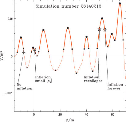
We can understand many of the remaining conditions through the work of Tegmark (2005), who considered a wide range of inflaton potentials using Gaussian random fields. The potential is of the form V(φ) = mv4f(φ/mh), where mv and mh are the characteristic vertical and horizontal mass scales, and f is a dimensionless function with values and derivatives of order unity. For initial conditions, Tegmark ‘sprays starting points randomly across the potential surface’. Figure 3 shows a typical inflaton potential.
|
Requirement I2 will be discussed in more detail below. For now we note that the inflaton must either begin or be driven into a region in which the SRA holds in order for the universe to inflate, as shown by the thick lines in Figure 3.
Requirement I3 comes rather naturally to inflation: Peacock (1999, p. 337) shows that the requirement that inflation produce a large number of e-folds is essentially the same as the requirement that inflation happen in the first place (i.e. SRA), namely φstart ≫ mPl. This assumes that the potential is relatively smooth, and that inflation terminates at a value of the field (φ) rather smaller than its value at the start. There is another problem lurking, however. If inflation lasts for ![]() 70 e-folds (for GUT scale inflation), then all scales inside the Hubble radius today started out with physical wavelength smaller than the Planck scale at the beginning of inflation (Brandenberger 2011). The predictions of inflation (especially the spectrum of perturbations), which use general relativity and a semi-classical description of matter, must omit relevant quantum gravitational physics. This is a major unknown — transplanckian effects may even prevent the onset of inflation.
70 e-folds (for GUT scale inflation), then all scales inside the Hubble radius today started out with physical wavelength smaller than the Planck scale at the beginning of inflation (Brandenberger 2011). The predictions of inflation (especially the spectrum of perturbations), which use general relativity and a semi-classical description of matter, must omit relevant quantum gravitational physics. This is a major unknown — transplanckian effects may even prevent the onset of inflation.
I4 is non-trivial. The inflaton potential (or, more specifically, the region of the inflaton potential which actually determines the evolution of the field) must have a region in which the slow-roll approximation does not hold. If the inflaton rolls into a local minimum (at φ0) while the SRA still holds (which requires V(φ0) ≫ mPl2/8π d2V/dφ2|φ0 Peacock 1999, p. 332), then inflation never ends.
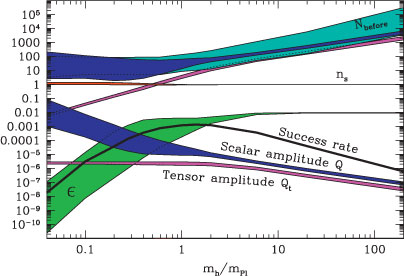
Tegmark (2005) asks what fraction of initial conditions for the inflaton field are successful, where success means that the universe inflates, inflation ends and the universes doesn’t thereafter meet a swift demise via a big crunch. The result is shown in Figure 4.
|
The thick black line shows the ‘success rate’ of inflation, for a model with mh/mPl as shown on the x-axis and mv = 0.001mPl. (This value has been chosen to maximise the probability that Q = Qobserved ≈ 2 × 10⁻⁵). The coloured curves show predictions for other cosmological parameters. The lower coloured regions are for mv =0.001mPl; the upper coloured regions are for mv = mh. The success rate peaks at ~0.1 percent, and drops rapidly as mh increases or decreases away from mPl. Even with a scalar field, inflation is far from guaranteed.
If inflation ends, we need its energy to be converted into ordinary matter (Condition I5). Inflation must not result in a universe filled with pure radiation or dark matter, which cannot form complex structures. Typically, the inflaton will to dump its energy into radiation. The temperature must be high enough to take advantage of baryon-number-violating physics for baryogenesis, and for γ + γ → particle + antiparticle reactions to create baryonic matter, but low enough not to create magnetic monopoles. With no physical model of the inflaton, the necessary coupling between the inflaton and ordinary matter/radiation is another postulate, but not an implausible one.
Requirement I6 brought about the downfall of ‘old’ inflation. When this version of inflation ended, it did so in expanding bubbles. Each bubble is too small to account for the homogeneity of the observed universe, and reheating only occurs when bubbles collide. As the space between the bubbles is still inflating, homogeneity cannot be achieved. New models of inflation have been developed which avoid this problem. More generally, the value of Q that results from inflation depends on the potential and initial conditions. We will discuss Q further in Section 4.5.
Perhaps the most pressing issue with inflation is hidden in requirement I2. Inflation is supposed to provide a dynamical explanation for the seemingly very fine-tuned initial conditions of the standard model of cosmology. But does inflation need special initial conditions? Can inflation act on generic initial conditions and produce the apparently fine-tuned universe we observe today? Hollands & Wald (2002b)15 contend not, for the following reason. Consider a collapsing universe. It would require an astonishing sequence of correlations and coincidences for the universe, in its final stages, to suddenly and coherently convert all its matter into a scalar field with just enough kinetic energy to roll to the top of its potential and remain perfectly balanced there for long enough to cause a substantial era of ‘deflation’. The region of final-condition-space that results from deflation is thus much smaller than the region that does not result from deflation. Since the relevant physics is time-reversible16, we can simply run the tape backwards and conclude that the initial-condition-space is dominated by universes that fail to inflate.
Readers will note the similarity of this argument to Penrose’s argument from Section 4.3. This intuitive argument can be formalised using the work of Gibbons, Hawking & Stewart (1987), who developed the canonical measure on the set of solutions of Einstein’s equation of General Relativity. A number of authors have used the Gibbons–Hawking–Stewart canonical measure to calculate the probability of inflation; see Hawking & Page (1988), Gibbons & Turok (2008) and references therein. We will summarise the work of Carroll & Tam (2010), who ask what fraction of universes that evolve like our universe since matter-radiation equality could have begun with inflation. Crucially, they consider the role played by perturbations:
Perturbations must be sub-dominant if inflation is to begin in the first place (Vachaspati & Trodden 1999), and by the end of inflation only small quantum fluctuations in the energy density remain. It is therefore a necessary (although not sufficient) condition for inflation to occur that perturbations be small at early times. …the fraction of realistic cosmologies that are eligible for inflation is therefore P(inflation) ≈10–6.6×10⁷.
Carroll & Tam casually note: ‘This is a small number’, and in fact an overestimate. A negligibly small fraction of universes that resemble ours at late times experience an early period of inflation. Carroll & Tam (2010) conclude that while inflation is not without its attractions (e.g. it may give a theory of initial conditions a slightly easier target to hit at the Planck scale), ‘inflation by itself cannot solve the horizon problem, in the sense of making the smooth early universe a natural outcome of a wide variety of initial conditions’. Note that this argument also shows that inflation, in and of itself, cannot solve the entropy problem17.
Let’s summarise. Inflation is a wonderful idea; in many ways it seems irresistible (Liddle 1995). However, we do not have a physical model, and even we had such a model, ‘although inflationary models may alleviate the ‘fine tuning’ in the choice of initial conditions, the models themselves create new ‘fine tuning’ issues with regard to the properties of the scalar field’ (Hollands & Wald 2002b). To pretend that the mere mention of inflation makes a life-permitting universe ‘100 percent’ inevitable (Foft 245) is naïve in the extreme, a cane toad solution. For a popular-level discussion of many of the points raised in our discussion of inflation, see Steinhardt (2011).
4.4.3 Inflation as a Case Study
Suppose that inflation did solve the fine-tuning of the density of the universe. Is it reasonable to hope that all fine-tuning cases could be solved in a similar way? We contend not, because inflation has a target. Let’s consider the range of densities that the universe could have had at some point in its early history. One of these densities is physically singled out as special — the critical density18. Now let’s note the range of densities that permit the existence of cosmic structure in a long-lived universe. We find that this range is very narrow. Very conveniently, this range neatly straddles the critical density.
We can now see why inflation has a chance. There is in fact a three-fold coincidence — A: the density needed for life, B: the critical density, and C: the actual density of our universe are all aligned. B and C are physical parameters, and so it is possible that some physical process can bring the two into agreement. The coincidence between A and B then creates the required anthropic coincidence (A and C). If, for example, life required a universe with a density (say, just after reheating) 10 times less than critical, then inflation would do a wonderful job of making all universes uninhabitable.
Inflation thus represents a very special case. Waiting inside the life-permitting range (L) is another physical parameter (p). Aim for p and you will get L thrown in for free. This is not true of the vast majority of fine-tuning cases. There is no known physical scale waiting in the life-permitting range of the quark masses, fundamental force strengths or the dimensionality of spacetime. There can be no inflation-like dynamical solution to these fine-tuning problems because dynamical processes are blind to the requirements of intelligent life.
What if, unbeknownst to us, there was such a fundamental parameter? It would need to fall into the life-permitting range. As such, we would be solving a fine-tuning problem by creating at least one more. And we would also need to posit a physical process able to dynamically drive the value of the quantity in our universe toward p.
4.5 The Amplitude of Primordial Fluctuations Q
Q, the amplitude of primordial fluctuations, is one of Martin Rees’ Just Six Numbers. In our universe, its value is Q ≈ 2 × 10⁻⁵, meaning that in the early universe the density at any point was typically within 1 part in 100 000 of the mean density. What if Q were different?
‘If Q were smaller than 10–6, gas would never condense into gravitationally bound structures at all, and such a universe would remain forever dark and featureless, even if its initial ‘mix’ of atoms, dark energy and radiation were the same as our own. On the other hand, a universe where Q were substantially larger than 10–5 — were the initial ‘ripples’ were replaced by large-amplitude waves — would be a turbulent and violent place. Regions far bigger than galaxies would condense early in its history. They wouldn’t fragment into stars but would instead collapse into vast black holes, each much heavier than an entire cluster of galaxies in our universe …Stars would be packed too close together and buffeted too frequently to retain stable planetary systems.’ (Rees 1999, p. 115)
Stenger has two replies:
‘[T]he inflationary model predicted that the deviation from smoothness should be one part in 100 000. This prediction was spectacularly verified by the Cosmic Background Explorer (COBE) in 1992.’ (Foft 106)
‘While heroic attempts by the best minds in cosmology have not yet succeeded in calculating the magnitude of Q, inflation theory successfully predicted the angular correlation across the sky that has been observed.’ (Foft 206)
Note that the first part of the quote contradicts the second part. We are first told that inflation predicts Q = 10–5, and then we are told that inflation cannot predict Q at all. Both claims are false. A given inflationary model will predict Q, and it will only predict a life-permitting value for Q if the parameters of the inflaton potential are suitably fine-tuned. As Turok (2002) notes, ‘to obtain density perturbations of the level required by observations …we need to adjust the coupling μ [for a power law potential μφn] to be very small, ~10–13 in Planck units. This is the famous fine-tuning problem of inflation’; see also Barrow & Tipler (1986, p. 437) and Brandenberger (2011). Rees’ life-permitting range for Q implies a fine-tuning of the inflaton potential of ~10–11 with respect to the Planck scale. Tegmark (2005, particularly figure 11) argues that on very general grounds we can conclude that life-permitting inflation potentials are highly unnatural.
Stenger’s second reply is to ask,
‘…is an order of magnitude fine-tuning? Furthermore, Rees, as he admits, is assuming all other parameters are unchanged. In the first case where Q is too small to cause gravitational clumping, increasing the strength of gravity would increase the clumping. Now, as we have seen, the dimensionless strength of gravity αG is arbitrarily defined. However, gravity is stronger when the masses involved are greater. So the parameter that would vary along with Q would be the nucleon mass. As for larger Q, it seems unlikely that inflation would ever result in large fluctuations, given the extensive smoothing that goes on during exponential expansion.’ (Foft 207)
There are a few problems here. We have a clear case of the flippant funambulist fallacy — the possibility of altering other constants to compensate the change in Q is not evidence against fine-tuning. Choose Q and, say, αG at random and you are unlikely to have picked a life-permitting pair, even if our universe is not the only life-permitting one. We also have a nice example of the cheap-binoculars fallacy. The allowed change in Q relative to its value in our universe (‘an order of magnitude’) is necessarily an underestimate of the degree of fine-tuning. The question is whether this range is small compared to the possible range of Q. Stenger seems to see this problem, and so argues that large values of Q are unlikely to result from inflation. This claim is false19. The upper blue region of Figure 4 shows the distribution of Q for the model of Tegmark (2005), using the ‘physically natural expectation’ mv = mh. The mean value of Q ranges from 10 to almost 10 000.
Note that Rees only varies Q in ‘Just Six Numbers’ because it is a popular level book. He and many others have extensively investigated the effect on structure formation of altering a number of cosmological parameters, including Q.
Tegmark & Rees (1998) were the first to calculate the range of Q which permits life, deriving the following limits for the case where ρΛ = 0:
where these quantities are defined in Table 1, except for the cosmic baryon density parameter Ωb, and we have omitted geometric factors of order unity. This inequality demonstrates the variety of physical phenomena, atomic, gravitational and cosmological, that must combine in the right way in order to produce a life-permitting universe. Tegmark & Rees also note that there is some freedom to change Q and ρΛ together.
Tegmark et al. (2006) expanded on this work, looking more closely at the role of the cosmological constant. We have already seen some of the results from this paper in Section 4.2.1. The paper considers 8 anthropic constraints on the 7 dimensional parameter space (α, β, mp, ρΛ, Q, ξ, ξbaryon). Figure 2 (bottom row) shows that the life-permitting region is boxed-in on all sides. In particular, the freedom to increase Q and ρΛ together is limited by the life-permitting range of galaxy densities.
Bousso et al. (2009) considers the 4-dimensional parameter space (β, Q, Teq, ρΛ), where Teq is the temperature if the CMB at matter-radiation equality. They reach similar conclusions to Rees et al.; see also Garriga et al. (1999); Bousso & Leichenauer (2009, 2010).
Garriga & Vilenkin (2006) discuss what they call the ‘Q catastrophe’: the probability distribution for Q across a multiverse typically increases or decreases sharply through the anthropic window. Thus, we expect that the observed value of Q is very likely to be close to one of the boundaries of the life-permitting range. The fact that we appear to be in the middle of the range leads Garriga & Vilenkin to speculate that the life-permitting range may be narrower than Tegmark & Rees (1998) calculated. For example, there may be a tighter upper bound due to the perturbation of comets by nearby stars and/or the problem of nearby supernovae explosions.
The interested reader is referred to the 90 scientific papers which cite Tegmark & Rees (1998), catalogued on the NASA Astrophysics Data System20.
The fine-tuning of Q stands up well under examination.
4.6 Cosmological Constant Λ
The cosmological constant problem is described in the textbook of Burgess & Moore (2006) as ‘arguably the most severe theoretical problem in high-energy physics today, as measured by both the difference between observations and theoretical predictions, and by the lack of convincing theoretical ideas which address it’. A well-understood and well-tested theory of fundamental physics (Quantum Field Theory — QFT) predicts contributions to the vacuum energy of the universe that are ~10120 times greater than the observed total value. Stenger’s reply is guided by the following principle:
‘Any calculation that disagrees with the data by 50 or 120 orders of magnitude is simply wrong and should not be taken seriously. We just have to await the correct calculation.’ (Foft 219)
This seems indistinguishable from reasoning that the calculation must be wrong since otherwise the cosmological constant would have to be fine-tuned. One could not hope for a more perfect example of begging the question. More importantly, there is a misunderstanding in Stenger’s account of the cosmological constant problem. The problem is not that physicists have made an incorrect prediction. We can use the term dark energy for any form of energy that causes the expansion of the universe to accelerate, including a ‘bare’ cosmological constant (see Barnes et al. 2005, for an introduction to dark energy). Cosmological observations constrain the total dark energy. QFT allows us to calculate a number of contributions to the total dark energy from matter fields in the universe. Each of these contributions turns out to be 10120 times larger than the total. There is no direct theory-vs.-observation contradiction as one is calculating and measuring different things. The fine-tuning problem is that these different independent contributions, including perhaps some that we don’t know about, manage to cancel each other to such an alarming, life-permitting degree. This is not a straightforward case of Popperian falsification.
Stenger outlines a number of attempts to explain the fine-tuning of the cosmological constant.
Supersymmetry: Supersymmetry, if it holds in our universe, would cancel out some of the contributions to the vacuum energy, reducing the required fine-tuning to one part in ~1050. Stenger admits the obvious — this isn’t an entirely satisfying solution — but there is a deeper reason to be sceptical of the idea that advances in particle physics could solve the cosmological constant problem. As Bousso (2008) explains:
…nongravitational physics depends only on energy differences, so the standard model cannot respond to the actual value of the cosmological constant it sources. This implies that ρΛ = 0 [i.e. zero cosmological constant] is not a special value from the particle physics point of view.
A particle physics solution to the cosmological constant problem would be just as significant a coincidence as the cosmological constant problem itself. Further, this is not a problem that appears only at the Planck scale. It is thus unlikely that quantum gravity will solve the problem. For example, Donoghue (2007) says
‘It is unlikely that there is technically natural resolution to the cosmological constant’s fine-tuning problem — this would require new physics at 10–3 eV. [Such attempts are] highly contrived to have new dynamics at this extremely low scale which modifies only gravity and not the other interactions.’
Zero Cosmological Constant: Stenger tries to show that the cosmological constant of general relativity should be defined to be zero. He says:
‘Only in general relativity, where gravity depends on mass/energy, does an absolute value of mass/energy have any consequence. So general relativity (or a quantum theory of gravity) is the only place where we can set an absolute zero of mass/ energy. It makes sense to define zero energy as the situation in which the source of gravity, the energy momentum tensor, and the cosmological constant are each zero.’
The second sentence contradicts the first. If gravity depends on the absolute value of mass/energy, then we cannot set the zero-level to our convenience. It is in particle physics, where gravity is ignorable, where we are free to define ‘zero’ energy as we like. In general relativity there is no freedom to redefine Λ. The cosmological constant has observable consequences that no amount of redefinition can disguise.
Stenger’s argument fails because of this premise: if (Tμν = 0 ⇒ Gμν = 0) then Λ = 0. This is true as a conditional, but Stenger has given no reason to believe the antecedent. Even if we associate the cosmological constant with the ‘SOURCE’ side of the equations, the antecedent nothing more than an assertion that the vacuum (Tμν = 0) doesn’t gravitate.
Even if Stenger’s argument were successful, it still wouldn’t solve the problem. The cosmological constant problem is actually a misnomer. This section has discussed the ‘bare’ cosmological constant. It comes purely from general relativity, and is not associated with any particular form of energy. The 120 orders-of-magnitude problem refers to vacuum energy associated with the matter fields of the universe. These are contributions to Tμν. The source of the confusion is the fact that vacuum energy has the same dynamical effect as the cosmological constant, so that observations measure an ‘effective’ cosmological constant: Λeff = Λbare +Λvacuum. The cosmological constant problem is really the vacuum energy problem. Even if Stenger could show that Λbare = 0, this would do nothing to address why Λeff is observed to be so much smaller than the predicted contributions to Λvacuum.
Quintessence: Stenger recognises that, even if he could explain why the cosmological constant and vacuum energy are zero, he still needs to explain why the expansion of the universe is accelerating. One could appeal to an as-yet-unknown form of energy called quintessence, which has an equation of state w = p/ρ that causes the expansion of the universe to accelerate21 (w < –1/3). Stenger concludes that:
…a cosmological constant is not needed for early universe inflation nor for the current cosmic acceleration. Note this is not vacuum energy, which is assumed to be identically zero, so we have no cosmological constant problem and no need for fine-tuning.
In reply, it is logically possible that the cause of the universe’s acceleration is not vacuum energy but some other form of energy. However, to borrow the memorable phrasing of Bousso (2008), if it looks, walks, swims, flies and quacks like a duck, then the most reasonable conclusion is not that it is a unicorn in a duck outfit. Whatever is causing the accelerated expansion of the universe quacks like vacuum energy. Quintessence is a unicorn in a duck outfit. We are discounting a form of energy with a plausible, independent theoretical underpinning in favour of one that is pure speculation.
The present energy density of quintessence must fall in the same life-permitting range that was required of the cosmological constant. We know the possible range of ρΛ because we have a physical theory of vacuum energy. What is the possible range of ρQ? We don’t know, because we have no well-tested, well-understood theory of quintessence. This is hypothetical physics. In the absence of a physical theory of quintessence, and with the hint (as discussed above) that gravitational physics must be involved, the natural guess for the dark energy scale is the Planck scale. In that case, ρQ is once again 120 orders of magnitude larger than the life-permitting scale, and we have simply exchanged the fine-tuning of the cosmological constant for the fine-tuning of dark energy.
Stenger’s assertion that there is no fine-tuning problem for quintessence is false, as a number of authors have pointed out. For example, Peacock (2007) notes that most models of quintessence in the literature specify its properties via a potential V(φ), and comments that ‘Quintessence …models do not solve the [cosmological constant] problem: the potentials asymptote to zero, even though there is no known symmetry that requires this’. Quintessence models must be fine-tuned in exactly the same way as the cosmological constant (see also Durrer & Maartens 2007).
Underestimating Λ: Stenger’s presentation of the cosmological constant problem fails to mention some of the reasons why this problem is so stubborn22. The first is that we know that the electron vacuum energy does gravitate in some situations. The vacuum polarisation contribution to the Lamb shift is known to give a nonzero contribution to the energy of the atom, and thus by the equivalence principle must couple to gravity. Similar effects are observed for nuclei. The puzzle is not just to understand why the zero point energy does not gravitate, but why it gravitates in some environments but not in vacuum. Arguing that the calculation of vacuum energy is wrong and can be ignored is naïve. There are certain contexts where we know that the calculation is correct.
Secondly, a dynamical selection mechanism for the cosmological constant is made difficult by the fact that only gravity can measure ρΛ, and ρΛ only becomes dynamically important quite recently in the history of the universe. Polchinski (2006) notes that many of the mechanisms aimed at selecting a small value for ρΛ — the Hawking-Hartle wavefunction, the de Sitter entropy and the Coleman-de Luccia amplitude for tunneling — can only explain why the cosmological constant vanishes in an empty universe.
Inflation creates another problem for would-be cosmological constant problem solvers. If the universe underwent a period of inflation in its earliest stages, then the laws of nature are more than capable of producing life-prohibiting accelerated expansion. The solution must therefore be rather selective, allowing acceleration in the early universe but severely limiting it later on. Further, the inflaton field is yet another contributor to the vacuum energy of the universe, and one with universe-accelerating pedigree. We can write a typical local minimum of the inflaton potential as: V(φ) = μ (φ – φ0)2 + V0. Post inflation, our universe settles into the minimum at φ = φ0, and the V0 term contributes to the effective cosmological constant. We have seen this point previously: the five- and six-pointed stars in Figure 4 show universes in which the value of V0 is respectively too negative and too positive for the post-inflationary universe to support life. If the calculation is wrong, then inflation is not a well-characterised theory. If the field does not cause the expansion of the universe to accelerate, then it cannot power inflation. There is no known symmetry that would set V0 = 0, because we do not know what the inflaton is. Most proposed inflation mechanisms operate near the Planck scale, so this defines the possible range of V0. The 120 order-of-magnitude fine-tuning remains.
The Principle of Mediocrity: Stenger discusses the multiverse solution to the cosmological constant problem, which relies on the principle of mediocrity. We will give a more detailed appraisal of this approach in Section 5. Here we note what Stenger doesn’t: an appeal to the multiverse is motivated by and dependent on the fine-tuning of the cosmological constant. Those who defend the multiverse solution to the cosmological constant problem are quite clear that they do so because they have judged other solutions to have failed. Examples abound:
-
‘There is not a single natural solution to the cosmological constant problem. …[With the discovery that Λ > 0] The cosmological constant problem became suddenly harder, as one could no longer hope for a deep symmetry setting it to zero.’ (Arkani-Hamed, Dimopoulos & Kachru 2005)
-
‘Throughout the years many people …have tried to explain why the cosmological constant is small or zero. The overwhelming consensus is that these attempts have not been successful.’ (Susskind 2005, p. 357)
-
‘No concrete, viable theory predicting ρΛ = 0 was known by 1998 [when the acceleration of the universe was discovered] and none has been found since.’ (Bousso 2008)
-
‘There is no known symmetry to explains why the cosmological constant is either zero or of order the observed dark energy.’ (Hall & Nomura 2008)
-
‘As of now, the only viable resolution of [the cosmological constant problem] is provided by the anthropic approach.’ (Vilenkin 2010)
See also Peacock (2007) and Linde & Vanchurin (2010), quoted above, and Susskind (2003).
Conclusion: There are a number of excellent reviews of the cosmological constant in the scientific literature (Weinberg 1989; Carroll 2001; Vilenkin 2003; Polchinski 2006, Durrer & Maartens 2007; Padmanabhan 2007; Bousso 2008). The calculations are known to be correct in other contexts and so are taken very seriously. Supersymmetry won’t help. The problem cannot be defined away. The most plausible small-vacuum-selecting mechanisms don’t work in a universe that contains matter. Particle physics is blind to the absolute value of the vacuum energy. The cosmological constant problem is not a problem only at the Planck scale and thus quantum gravity is unlikely to provide a solution. Quintessence and the inflaton field are just more fields whose vacuum state must be sternly commanded not to gravitate, or else mutually balanced to an alarming degree.
There is, of course, a solution to the cosmological problem. There is some reason — some physical reason — why the large contributions to the vacuum energy of the universe don’t make it life-prohibiting. We don’t currently know what that reason is, but scientific papers continue to be published that propose new solutions to the cosmological constant problem (e.g. Shaw & Barrow 2011). The point is this: however many ways there are of producing a life-permitting universe, there are vastly many more ways of making a life-prohibiting one. By the time we discover how our universe solves the cosmological constant problem, we will have compiled a rather long list of ways to blow a universe to smithereens, or quickly crush it into oblivion. Amidst the possible universes, life-permitting ones are exceedingly rare. This is fine-tuning par excellence.
4.7 Stars
Stars have two essential roles to play in the origin and evolution of intelligent life. They synthesise the elements needed by life — big bang nucleosynthesis provides only hydrogen, helium and lithium, which together can form just two chemical compounds (H2 and LiH). By comparison, Gingerich (2008) notes that the carbon and hydrogen alone can be combined into around 2300 different chemical compounds. Stars also provide a long-lived, low-entropy source of energy for planetary life, as well as the gravity that holds planets in stable orbits. The low-entropy of the energy supplied by stars is crucial if life is to ‘evade the decay to equilibrium’ (Schrödinger 1992).
4.7.1 Stellar Stability
Stars are defined by the forces that hold them in balance. The crushing force of gravity is held at bay by thermal and radiation pressure. The pressure is sourced by thermal reactions at the centre of the star, which balance the energy lost to radiation. Stars thus require a balance between two very different forces — gravity and the strong force — with the electromagnetic force (in the form of electron scattering opacity) providing the link between the two.
There is a window of opportunity for stars — too small and they won’t be able to ignite and sustain nuclear fusion at their cores, being supported against gravity by degeneracy rather than thermal pressure; too large and radiation pressure will dominate over thermal pressure, allowing unstable pulsations. Barrow & Tipler (1986, p. 332) showed that this window is open when,
where the first expression uses the more exact calculation of the right-hand-side by Adams (2008), and the second expression uses Barrow & Tipler’s approximation for the minimum nuclear ignition temperature Tnuc ~ ηα2mp, where η ≈ 0.025 for hydrogen burning. Outside this range, stars are not stable: anything big enough to burn is big enough to blow itself apart. Adams (2008) showed there is another criterion that must be fulfilled for stars have a stable burning configuration,
where  is a composite parameter related to nuclear reaction rates, and we have specialised equation 44 of Adams to the case where stellar opacity is due to Thomson scattering.
Adams combines these constraints in (G, α,  ) parameter space, holding all other parameters constant, as shown in Figure 5. Below the solid line, stable stars are possible. The dashed (dotted) line shows the corresponding constraint for universes in which
  is increased (decreased) by a factor of 100. Adams remarks that ‘within the parameter space shown, which spans 10 orders of magnitude in both α and G, about one-fourth of the space supports the existence of stars’.
|
 is increased (decreased) by a factor of 100. Note that the axes are logarithmic and span 10 orders of magnitude. Figure from
 Stenger (Foft 243) cites Adams’ result, but crucially omits the modifier shown. Adams makes no attempt to justify the limits of parameter space as he has shown them. Further, there is no justification of the use of logarithmic axes, which significantly affects the estimate of the probability23. The figure of ‘one-fourth’ is almost meaningless — given any life-permitting region, one can make it equal one-fourth of parameter space by chopping and changing said space. This is a perfect example of the cheap-binoculars fallacy. If one allows G to increase until gravity is as strong as the strong force (αG ≈ αs ≈ 1), and uses linear rather than logarithmic axes, the stable-star-permitting region occupies ~ 10–38 of parameter space. Even with logarithmic axes, fine-tuning cannot be avoided — zero is a possible value of G, and thus is part of parameter space. However, such a universe is not life-permitting, and so there is a minimum life-permitting value of G. A logarithmic axis, by placing G = 0 at negative infinity, puts an infinitely large region of parameter space outside of the life-permitting region. Stable stars would then require infinite fine-tuning. Note further that the fact that our universe (the triangle in Figure 5) isn’t particularly close to the life-permitting boundary is irrelevant to fine-tuning as we have defined it. We conclude that the existence of stable stars is indeed a fine-tuned property of our universe.
4.7.2 The Hoyle Resonance
One of the most famous examples of fine-tuning is the Hoyle resonance in carbon. Hoyle reasoned that if such a resonance level did not exist at just the right place, then stars would be unable to produce the carbon required by life24.
Is the Hoyle resonance (called the 0+ level) fine-tuned? Stenger quotes the work of Livio et al. (1989), who considered the effect on the carbon and oxygen production of stars when the 0+ level is shifted. They found one could increase the energy of the level by 60 keV without effecting the level of carbon production. Is this a large change or a small one? Livio et al. (1989) ask just this question, noting the following. The permitted shift represents a 0.7% change in the energy of the level itself. It is 3% of the energy difference between the 0+ level and the next level up in the carbon nucleus (3–). It is 16% of the difference between the energy of the 0+ state and the energy of three alpha particles, which come together to form carbon.
Stenger argues that this final estimate is the most appropriate one, quoting from Weinberg (2007):
‘We know that even-even nuclei have states that are well described as composites of α particles. One such state is the ground state of Be8, which is unstable against fission into two α particles.The same α–α potential that produces that sort of unstable state in Be8 could naturally be expected to produce an unstable state in C12 that is essentially a composite of three α particles, and that therefore appears as a low-energy resonance in α-Be8 reactions. So the existence of this state does not seem to me to provide any evidence of fine tuning.’
As Cohen (2008) notes, the 0+ state is known as a breathing mode; all nuclei have such a state.
However, we are not quite done with assessing this fine-tuning case. The existence of the 0+ level is not enough. It must have the right energy, and so we need to ask how the properties of the resonance level, and thus stellar nucleosynthesis, change as we alter the fundamental constants. Oberhummer, Csótó & Schlattl (2000a)25 have performed such calculations, combining the predictions of a microscopic 12-body, three-alpha cluster model of 12C (as alluded to by Weinberg) with a stellar nucleosynthesis code. They conclude that:
Even with a change of 0.4% in the strength of [nucleon-nucleon] force, carbon-based life appears to be impossible, since all the stars then would produce either almost solely carbon or oxygen, but could not produce both elements.
Schlattl et al. (2004), by the same group, noted an important caveat on their previous result. Modelling the later, post-hydrogen-burning stages of stellar evolution is difficult even for modern codes, and the inclusion of He-shell flashes seems to lessen the degree of fine-tuning of the Hoyle resonance.
Ekström et al. (2010) considered changes to the Hoyle resonance in the context of Population III stars. These first-generation stars play an important role in the production of the elements needed by life. Ekström et al. (2010) place similar limits to Oberhummer et al. (2000a) on the nucleon-nucleon force, and go further by translating these limits into limits on the fine-structure constant, α. A fractional change in α of one part in 105 would change the energy of the Hoyle resonance enough that stars would contain carbon or oxygen at the end of helium burning but not both.
There is again reason to be cautious, as stellar evolution has not been followed to the very end of the life of the star. Nevertheless, these calculations are highly suggestive — the main process by which carbon and oxygen are synthesised in our universe is drastically curtailed by a tiny change in the fundamental constants. Life would need to hope that sufficient carbon and oxygen are synthesized in other ways, such as supernovae. We conclude that Stenger has failed to turn back the force of this fine-tuning case. The ability of stars in our universe to produce both carbon and oxygen seems to be a rare talent.
4.8 Forces and Masses
In Chapters 7–10, Stenger turns his attention to the strength of the fundamental forces and the masses of the elementary particles. These quantities are among the most discussed in the fine-tuning literature, beginning with Carter (1974), Carr & Rees (1979) and Barrow & Tipler (1986). Figure 6 shows in white the life-permitting region of (α, β) (left) and (α, αs) (right) parameter space26. The axes are scaled like arctan (log10[x]), so that the interval [0, ∞] maps onto a finite range. The blue cross shows our universe. This figure is similar to those of Tegmark (1998). The various regions illustrated are as follows:

|
-
For hydrogen to exist — to power stars and form water and organic compounds — we must have me < mn – mp. Otherwise, the electron will be captured by the proton to form a neutron (Hogan 2006; Damour & Donoghue 2008).
-
For stable atoms, we need the radius of the electron orbit to be significantly larger than the nuclear radius, which requires αβ/αs ≪ 1 (Barrow & Tipler 1986, p. 320). The region shown is αβ/αs < 1/1000, which Stenger adopts (Foft 244).
-
We require that the typical energy of chemical reactions is much smaller than the typical energy of nuclear reactions. This ensures that the atomic constituents of chemical species maintain their identity in chemical reactions. This requires α2β/αs2 ≪ 1 (Barrow & Tipler 1986, p. 320). The region shown is α2β/αs2 < 1/1000.
-
Unless β1/4 ≪ 1, stable ordered molecular structures (like chromosomes) are not stable. The atoms will too easily stray from their place in the lattice and the substance will spontaneously melt (Barrow & Tipler 1986, p. 305). The region shown is β1/4 < 1/3.
-
The stability of the proton requires α
 (md – mu)/141 MeV, so that the extra electromagnetic mass-energy of a proton relative to a neutron is more than counter-balanced by the bare quark masses (Hogan 2000; Hall & Nomura 2008).
 -
Unless α ≪ 1, the electrons in atoms and molecules are unstable to pair creation (Barrow & Tipler 1986, p. 297). The limit shown is α < 0.2. A similar constraint is calculated by Lieb & Yau (1988).
-
As in Equation 4, stars will not be stable unless β
 α2/100.
 -
Unless αs/αs,0
1.003 + 0.031α/α0 (Davies 1972), the diproton has a bound state, which affects stellar burning and big bang nucleosynthesis. (Note, however, the caveats mentioned in Footnote 9.) -
Unless αs
0.3α1/2, carbon and all larger elements are unstable (Barrow & Tipler 1986, p. 326). -
Unless αs/αs,0
0.91 (Davies 1972), the deuteron is unstable and the main nuclear reaction in stars (pp) does not proceed. A similar effect would be achieved27 unless md – mu + me < 3.4 MeV which makes the pp reaction energetically unfavourable (Hogan 2000). This region is numerically very similar to Region 1 in the left plot; the different scaling with the quark masses is illustrated in Figure 7.
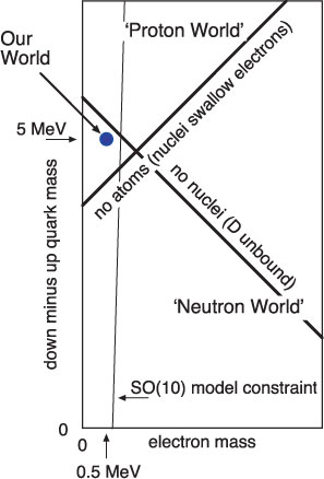
|
-
The grey stripe on the left of each plot shows where α < αG, rendering electric forces weaker than gravitational ones.
-
To the left of our universe (the blue cross) is shown the limit of Adams (2008) on stellar stability, Equation 5. The limit shown is α > 7.3 × 10⁻⁵, as read off figure 5 of Adams (2008). The dependence on β and αs has not been calculated, and so only the limit for the case when these parameters take the value they have in our universe is shown28.
-
The upper limit shown in the right plot of Figure 6 is the result of MacDonald & Mullan (2009) that the amount of hydrogen left over from big bang nucleosynthesis is significantly diminished when αs > 0.27. Note that this is weaker than the condition that the diproton be bound. The dependence on α has not been calculated, so only a 1D limit is shown.
-
The dashed line in the left plot shows a striking coincidence discussed by Carter (1974), namely α12β4 ~ αG. Near this line, the universe will contain both radiative and convective stars. Carter conjectured that life may require both types for reasons pertaining to planet formation and supernovae. This reason is somewhat dubious, but a better case can be made. The same coincidence can be shown to ensure that the surface temperature of stars is close to ‘biological temperature’ (Barrow & Tipler 1986, p. 338). In other words, it ensures that the photons emitted by stars have the right energy to break chemical bonds. This permits photosynthesis, allowing electromagnetic energy to be converted into and stored as chemical energy in plants. However, it is not clear how close to the line a universe must be to be life-permitting, and the calculation considers only radiation dominated stars.
-
The left solid line shows the lower limit α > 1/180 for a grand-unified theory to unify no higher than the Planck scale. The right solid line shows the boundary of the condition that protons be stable on stellar timescales (β2 > α (αG exp α–1)–1, Barrow & Tipler 1986, p. 358). These limits are based on Grand Unified Theories (GUT) and thus somewhat more speculative. We will say more about GUTs below.
-
The triple-alpha constraint is not shown. The constraint on carbon production from Ekström et al. (2010) is –3.5 × 10⁻⁵
Δα/α +1.8 × 10⁻⁵, as discussed in Section 4.7.2. Note also the caveats discussed there. This only considers the change in α i.e. horizontally, and the life-permitting region is likely to be a 2D strip in both the (α, β) and (α, αs) plane. As this strip passes our universe, its width in the x-direction is one-thousandth of the width of one of the vertical black lines. -
The limits placed on α and β from chemistry are weaker than the constraints listed above. If we consider the nucleus as fixed in space, then the time-independent, non-relativistic Schrödinger equation scales with α2me i.e. the relative energy and properties of the energy levels of electrons (which determine chemical bonding) are unchanged (Barrow & Tipler 1986, p. 533). The change in chemistry with fundamental parameters depends on the accuracy of the approximations of an infinite mass nucleus and non-relativistic electrons. This has been investigated by King et al. (2010) who considered the bond angle and length in water, and the reaction energy of a number of organic reactions. While ‘drastic changes in the properties of water’ occur for α
0.08 and β 0.054, it is difficult to predict what impact these changes would have on the origin and evolution of life.
Note that there are four more constraints on α, me and mp from the cosmological considerations of Tegmark et al. (2006), as discussed in Section 4.2. There are more cases of fine-tuning to be considered when we expand our view to consider all the parameters of the standard model of particle physics.
Agrawal et al. (1998a, b) considered the life-permitting range of the Higgs mass parameter μ2, and the corresponding limits on the vacuum expectation value, v = (–μ2/λ)1/2, which takes the value 246 GeV =2 × 10–17mPl in our universe. After exploring the range [–mPl, mPl], they find that ‘only for values in a narrow window is life likely to be possible’. In Planck units, the relevant limits are: for v > 4 × 10–17, the deuteron is strongly unstable (see point 10 above); for v > 10–16, the neutron is heavier than the proton by more than the nucleon’s binding energy, so that even bound neutrons decay into protons and no nuclei larger than hydrogen are stable; for v > 2 × 10–14, only the Δ++ particle is stable and the only stable nucleus has the chemistry of helium; for v ![]() 2 × 10–19, stars will form very slowly (~1017 yr) and burn out very quickly (~1 yr), and the large number of stable nucleon species may make nuclear reactions so easy that the universe contains no light nuclei. Damour & Donoghue (2008) refined the limits of Agrawal et al. by considering nuclear binding, concluding that unless 0.78 × 10⁻¹⁷ < v < 3.3 × 10⁻¹⁷ hydrogen is unstable to the reaction p + e → n + ν (if v is too small) or else there is no nuclear binding at all (if v is too large).
2 × 10–19, stars will form very slowly (~1017 yr) and burn out very quickly (~1 yr), and the large number of stable nucleon species may make nuclear reactions so easy that the universe contains no light nuclei. Damour & Donoghue (2008) refined the limits of Agrawal et al. by considering nuclear binding, concluding that unless 0.78 × 10⁻¹⁷ < v < 3.3 × 10⁻¹⁷ hydrogen is unstable to the reaction p + e → n + ν (if v is too small) or else there is no nuclear binding at all (if v is too large).
Jeltema & Sher (1999) combined the conclusions of Agrawal et al. and Oberhummer et al. (2000a) to place a constraint on the Higgs vev from the fine-tuning of the Hoyle resonance (Section 4.7.2). They conclude that a 1% change in v from its value in our universe would significantly affect the ability of stars to synthesise both oxygen and carbon. Hogan (2006) reached a similar conclusion: ‘In the absence of an identified compensating factor, increases in [v/ΛQCD] of more than a few percent lead to major changes in the overall cosmic carbon creation and distribution’. Remember, however, the caveats of Section 4.7.2: it is difficult to predict exactly when a major change becomes a life-prohibiting change.
There has been considerable attention given to the fine-tuning of the masses of fundamental particles, in particular mu, md and me. We have already seen the calculation of Barr & Khan (2007) in Figure 2, which shows the life-permitting region of the mu–md plane. Hogan (2000) was one of the first to consider the fine-tuning of the quark masses (see also Hogan 2006). Such results have been confirmed and extended by Damour & Donoghue (2008), Hall & Nomura (2008) and Bousso et al. (2009).
Jaffe et al. (2009) examined a different slice through parameter space, varying the masses of the quarks while ‘holding as much as possible of the rest of the Standard Model phenomenology constant’ [emphasis original]. In particular, they fix the electron mass, and vary ΛQCD so that the average mass of the lightest baryon(s) is 940 MeV, as in our universe. These restrictions are chosen to make the characterisation of these other universes more certain. Only nuclear stability is considered, so that a universe is deemed congenial if both carbon and hydrogen are stable. The resulting congenial range is shown in Figure 8. The height of each triangle is proportional to the total mass of the three lightest quarks: mT = mu + md + ms; the centre triangle has mT as in our universe. The perpendicular distance from each side represents the mass of the u, d and s quarks. The lower green region shows universes like ours with two light quarks (mu, md ≪ ms), and is bounded above by the stability of some isotope of hydrogen (in this case, tritium) and below by the corresponding limit for carbon 10C, (–21.80 MeV < mp – mn < 7.97 MeV). The smaller green strip shows a novel congenial region, where there is one light quark (md ≪ ms ≈ mu). This congeniality band has half the width of the band in which our universe is located. The red regions are uncongenial, while white regions show where it is uncertain where the red-green boundary should lie. Note two things about the larger triangle on the right. Firstly, the smaller congenial band detaches from the edge of the triangle for mT ![]() 1.22mT,0 as the lightest baryon is the Δ++, which would be incapable of forming nuclei. Secondly, and most importantly for our purposes, the absolute width of the green regions remains the same, and thus the congenial fraction of the space decreases approximately as 1/mT. Moving from the centre (mT = mT,0) to the right (mT = 2mT,0) triangle of Figure 8, the congenial fraction drops from 14% to 7%. Finally, ‘congenial’ is almost certainly a weaker constraint than ‘life-permitting’, since only nuclear stability is investigated. For example, a universe with only tritium will have an element which is chemically very similar to hydrogen, but stars will not have 1H as fuel and will therefore burn out significantly faster.
1.22mT,0 as the lightest baryon is the Δ++, which would be incapable of forming nuclei. Secondly, and most importantly for our purposes, the absolute width of the green regions remains the same, and thus the congenial fraction of the space decreases approximately as 1/mT. Moving from the centre (mT = mT,0) to the right (mT = 2mT,0) triangle of Figure 8, the congenial fraction drops from 14% to 7%. Finally, ‘congenial’ is almost certainly a weaker constraint than ‘life-permitting’, since only nuclear stability is investigated. For example, a universe with only tritium will have an element which is chemically very similar to hydrogen, but stars will not have 1H as fuel and will therefore burn out significantly faster.

|
Tegmark, Vilenkin & Pogosian (2005) studied anthropic constraints on the total mass of the three neutrino species. If ∑mν ![]() 1 eV then galaxy formation is significantly suppressed by free streaming. If ∑mν is large enough that neutrinos are effectively another type of cold dark matter, then the baryon fraction in haloes would be very low, affecting baryonic disk and star formation. If all neutrinos are heavy, then neutrons would be stable and big bang nucleosynthesis would leave no hydrogen for stars and organic compounds. This study only varies one parameter, but its conclusions are found to be ‘rather robust’ when ρΛ is also allowed to vary (Pogosian & Vilenkin 2007).
1 eV then galaxy formation is significantly suppressed by free streaming. If ∑mν is large enough that neutrinos are effectively another type of cold dark matter, then the baryon fraction in haloes would be very low, affecting baryonic disk and star formation. If all neutrinos are heavy, then neutrons would be stable and big bang nucleosynthesis would leave no hydrogen for stars and organic compounds. This study only varies one parameter, but its conclusions are found to be ‘rather robust’ when ρΛ is also allowed to vary (Pogosian & Vilenkin 2007).
There are a number of tentative anthropic limits relating to baryogenesis. Baryogenesis is clearly crucial to life — a universe which contained equal numbers of protons and antiprotons at annihilation would only contain radiation, which cannot form complex structures. However, we do not currently have a well-understood and well-tested theory of baryogenesis, so caution is advised. Gould (2010) has argued that three or more generations of quarks and leptons are required for CP violation, which is one of the necessary conditions for baryogenesis (Sakharov 1967; Cahn 1996; Schellekens 2008). Hall & Nomura (2008) state that v/ΛQCD ~ 1 is required ‘so that the baryon asymmetry of the early universe is not washed out by sphaleron effects’ (see also Arkani-Hamed et al. 2005).
Harnik, Kribs & Perez (2006) attempted to find a region of parameter space which is life-permitting in the absence of the weak force. With some ingenuity, they plausibly discovered one, subject to the following conditions. To prevent big bang nucleosynthesis burning all hydrogen to helium in the early universe, they must use a ‘judicious parameter adjustment’ and set the baryon to photon radio ηb = 4 × 10–12. The result is a substantially increased abundance of deuterium, ~10% by mass. ΛQCD and the masses of the light quarks and leptons are held constant, which means that the nucleon masses and thus nuclear physics is relatively unaffected (except, of course, for beta decay) so long as we ‘insist that the weakless universe is devoid of heavy quarks’ to avoid problems relating to the existence of stable baryons29 Λc+, Λb0 and Λt+. Since v ~ mPl in the weakless universe, holding the light fermion masses constant requires the Yukawa parameters (Γe, Γu, Γd, Γs) must all be set by hand to be less than 10–20 (Feldstein et al. 2006). The weakless universe requires Ωbaryon/Ωdark matter ~ 10–3, 100 times less than in our universe. This is very close to the limit of Tegmark et al. (2006), who calculated that unless Ωbaryon/Ωdark matter ![]() 5 × 10⁻³, gas will not cool into galaxies to form stars. Galaxy formation in the weakless universe will thus be considerably less efficient, relying on rare statistical fluctuations and cooling via molecular viscosity. The proton-proton reaction which powers stars in our universe relies on the weak interaction, so stars in the weakless universe burn via proton-deuterium reactions, using deuterium left over from the big bang. Stars will burn at a lower temperature, and probably with shorter lifetimes. Stars will still be able to undergo accretion supernovae (Type 1a), but the absence of core-collapse supernovae will seriously affect the oxygen available for planet formation and life (Clavelli & White 2006). Only ~1% of the oxygen in our universe comes from accretion supernovae. It is then somewhat optimistic to claim that (Gedalia, Jenkins & Perez 2011),
5 × 10⁻³, gas will not cool into galaxies to form stars. Galaxy formation in the weakless universe will thus be considerably less efficient, relying on rare statistical fluctuations and cooling via molecular viscosity. The proton-proton reaction which powers stars in our universe relies on the weak interaction, so stars in the weakless universe burn via proton-deuterium reactions, using deuterium left over from the big bang. Stars will burn at a lower temperature, and probably with shorter lifetimes. Stars will still be able to undergo accretion supernovae (Type 1a), but the absence of core-collapse supernovae will seriously affect the oxygen available for planet formation and life (Clavelli & White 2006). Only ~1% of the oxygen in our universe comes from accretion supernovae. It is then somewhat optimistic to claim that (Gedalia, Jenkins & Perez 2011),

where {αus} ({αweakless}) represents the set of parameters of our (the weakless) universe. Note that, even if Equation 6 holds, the weakless universe at best opens up a life-permitting region of parameter space of similar size to the region in which our universe resides. The need for a life-permitting universe to be fine-tuned is not significantly affected.
4.8.1 The Origin of Mass
Let’s consider Stenger’s responses to these cases of fine-tuning.
Higgs and Hierarchy:
‘Electrons, muons, and tauons all pick up mass by the Higgs mechanism. Quarks must pick up some of their masses this way, but they obtain most of their masses by way of the strong interaction …All these masses are orders of magnitude less than the Planck mass, and no fine-tuning was necessary to make gravity much weaker than electromagnetism. This happened naturally and would have occurred for a wide range of mass values, which, after all, are just small corrections to their intrinsically zero masses. …In any case, these small mass corrections do not call for any fine-tuning or indicate that our universe is in any way special. …[mpme/m2Pl] is so small because the masses of the electron and the protons are so small compared to the Planck mass, which is the only ‘natural’ mass you can form from the simplest combination of fundamental constants.’ (Foft 154,156,175)
Stenger takes no cognizance of the hierarchy and flavour problems, widely believed to be amongst the most important problems of particle physics:
Lisa Randal: ‘The universe seems to have two entirely different mass scales, and we don’t understand why they are so different. There’s what’s called the Planck scale, which is associated with gravitational interactions. It’s a huge mass scale …1019 GeV. Then there’s the electroweak scale, which sets the masses for the W and Z bosons. [~100 GeV] …So the hierarchy problem, in its simplest manifestation, is how can you have these particles be so light when the other scale is so big.’ (Taubes 2002)
Frank Wilzcek: ‘We have no …compelling idea about the origin of the enormous number [mPl/me] = 2.4 × 10²². If you would like to humble someone who talks glibly about the Theory of Everything, just ask about it, and watch ‘em squirm.’ (Wilczek 2005)
Leonard Susskind: ‘The up- and down-quarks are absurdly light. The fact that they are roughly twenty thousand times lighter than particles like the Z-boson …needs an explanation. The Standard Model has not provided one. Thus, we can ask what the world would be like is the up- and down-quarks were much heavier than they are. Once again — disaster!’ (Susskind 2005, p. 176)
The problem is as follows. The mass of a fundamental particle in the standard model is set by two factors:  , where i labels the particle species, Γi is called the Yukawa parameter (e.g. electron: Γe ≈ 2.9 ×10⁻⁶, up quark: Γu ≈ 1.4 × 10⁻⁵, down quark: Γd ≈2.8 × 10⁻⁵), and v is the Higgs vacuum expectation value, which is the same for all particles (see Burgess & Moore 2006, for an introduction). Note that, contra Stenger, the bare masses of the quarks are not related to the strong force30.
There are, then, two independent ways in which the masses of the basic constituents of matter are surprisingly small: v = 2 × 10–17mPl, which ‘is so notorious that it’s acquired a special name — the Hierarchy Problem — and spawned a vast, inconclusive literature’ (Wilczek 2006a), and Γi ~ 10–6, which implies that, for example, the electron mass is unnaturally smaller than its (unnaturally small) natural scale set by the Higgs condensate (Wilczek 2007, p. 53) . This is known as the flavour problem.
Let’s take a closer look at the hierarchy problem. The problem (as ably explained by Martin 1998) is that the Higgs mass (squared) mH2 receives quantum corrections from the virtual effects of every particle that couples, directly or indirectly, to the Higgs field. These corrections are enormous — their natural scale is the Planck scale, so that these contributions must be fine-tuned to mutually cancel to one part in mPl2/mH2 ≈ 1032. Stenger’s reply is to say that:
‘…the masses of elementary particles are small compared to the Planck mass. No fine-tuning is required. Small masses are a natural consequence of the origin of mass. The masses of elementary particles are essentially small corrections to their intrinsically zero masses.’ (Foft 187)
Here we see the problem itself presented as its solution. It is precisely the smallness of the quantum corrections wherein the fine-tuning lies. If the Planck mass is the ‘natural’ (Foft 175) mass scale in physics, then it sets the scale for all mass terms, corrections or otherwise. Just calling them ‘small’ doesn’t explain anything.
Attempts to solve the hierarchy problem have driven the search for theories beyond the standard model: technicolor, the supersymmetric standard model, large extra dimensions, warped compactifications, little Higgs theories and more — even anthropic solutions (Arkani-Hamed & Dimopoulos 2005; Arkani-Hamed et al. 2005; Feldstein et al. 2006; Hall & Nomura 2008, 2010; Donoghue et al. 2010). Perhaps the most popular option is supersymmetry, whereby the Higgs mass scale doesn’t receive corrections from mass scales above the supersymmetry-breaking scale ΛSM due to equal and opposite contributions from supersymmetric partners. This ties v to ΛSM. The question now is: why is ΛSM ≪ mPl? This is known in the literature as ‘the μ-problem’, in reference to the parameter in the supersymmetric potential that sets the relevant mass scale. The value of μ in our universe is probably ~102–103 GeV. The natural scale for μ is mPl, and thus we still do not have an explanation for why the quark and lepton masses are so small. Low-energy supersymmetry does not by itself explain the magnitude of the weak scale, though it protects it from radiative correction (Barr & Khan 2007). Solutions to the μ-problem can be found in the literature (see Martin 1998, for a discussion and references).
We can draw some conclusions. First, Stenger’s discussion of the surprising lightness of fundamental masses is woefully inadequate. To present it as a solved problem of particle physics is a gross misrepresentation of the literature. Secondly, smallness is not sufficient for life. Recall that Damour & Donoghue (2008) showed that unless 0.78 × 10⁻¹⁷ < v/mPl < 3.3 × 10⁻¹⁷, the elements are unstable. The masses must be sufficiently small but not too small. Finally, suppose that the LHC discovers that supersymmetry is a (broken) symmetry of our universe. This would not be the discovery that the universe could not have been different. It would not be the discovery that the masses of the fundamental particles must be small. It would at most show that our universe has chosen a particularly elegant and beautiful way to be life-permitting.
QCD and Mass-Without-Mass: The bare quark masses, discussed above, only account for a small fraction of the mass of the proton and neutron. The majority of the other 95% comes from the strong force binding energy of the valence quarks. This contribution can be written as aΛQCD, where a ≈ 4 is a dimensionless constant determined by quantum chromodynamics (QCD). In Planck units, ΛQCD ≈ 10–20mPl. The question ‘why is gravity so feeble?’ (i.e. αG ≪ 1) is at least partly answered if we can explain why ΛQCD ≪ mPl. Unlike the bare masses of the quarks and leptons, we can answer this question from within the standard model.
The strength of the strong force αs is a function of the energy of the interaction. ΛQCD is the mass-energy scale at which αs diverges. Given that the strength of the strong force runs very slowly (logarithmically) with energy, there is a exponential relationship between ΛQCD and the scale of grand unification mU:
where b is a constant of order unity. Thus, if the QCD coupling is even moderately small at the unification scale, the QCD scale will be a long way away. To make this work in our universe, we need αs(mU) ≈ 1/25, and mU ≈ 1016 GeV (De Boer & Sander 2004). The calculation also depends on the spectrum of quark flavours; see Hogan (2000), Wilczek (2002) and Schellekens (2008, Appendix C).
As an explanation for the value of the proton and neutron mass in our universe, we aren’t done yet. We don’t know how to calculate the αs(mU), and there is still the puzzle of why the unification scale is three orders of magnitude below the Planck scale. From a fine-tuning perspective, however, this seems to be good progress, replacing the major miracle ΛQCD/mPl ~ 10–20 with a more minor one, αs(mU) ~ 10–1. Such explanations have been discussed in the fine-tuning literature for many years (Carr & Rees 1979; Hogan 2000).
Note that this does not completely explain the smallness of the proton mass, since mp is the sum of a number of contributions: QCD (ΛQCD), electromagnetism, the masses of the valence quarks (mu and md), and the mass of the virtual quarks, including the strange quark, which makes a surprisingly large contribution to the mass of ordinary matter. We need all of the contributions to be small in order for mp to be small.
Potential problems arise when we need the proton mass to fall within a specific range, rather than just be small, since the proton mass depends very sensitively (exponentially) on αU. For example, consider Region 4 in Figure 6, β1/4 ≪ 1. The constraint shown, β1/4 < 1/3 would require a 20-fold decrease in the proton mass to be violated, which (using Equation 7) translates to decreasing αU by ~0.003. Similarly, Region 7 will be entered if αU is increased31 by ~0.008. We will have more to say about grand unification and fine-tuning below. For the moment, we note that the fine-tuning of the mass of the proton can be translated into anthropic limits on GUT parameters.
Protons, Neutrons, Electrons: We turn now to the relative masses of the three most important particles in our universe: the proton, neutron and electron, from which atoms are made. Consider first the ratio of the electron to the proton mass, β, of which Stenger says:
‘…we can argue that the electron mass is going to be much smaller than the proton mass in any universe even remotely like ours. …The electron gets its mass by interacting electroweakly with the Higgs boson. The proton, a composite particle, gets most of its mass from the kinetic energies of gluons swirling around inside. They interact with one another by way of the strong interaction, leading to relatively high kinetic energies. Unsurprisingly, the proton’s mass is much higher than the electron’s and is likely to be so over a large region of parameter space. …The electron mass is much smaller than the proton mass because it gets its mass solely from the electroweak Higgs mechanism, so being less than 1.29 MeV is not surprising and also shows no sign of fine-tuning.’ (Foft 164,178)
Remember that fine-tuning compares the life-permitting range of a parameter with the possible range. Foft has compared the electron mass in our universe with the electron mass in universes ‘like ours’, thus missing the point entirely.
In terms of the parameters of the standard model, β ≡ me/mp ≈ Γev/aΛQCD. The smallness of β is thus quite surprising, since the ratio of the natural mass scale of the electron and the proton is v/ΛQCD ≈ 103. The smallness of β stems from the fact that the dimensionless constant for the proton is of order unity (a ≈ 4), while the Yukawa constant for the electron is unnaturally small Γe ≈ 10–6. Stenger’s assertion that the Higgs mechanism (with mass scale 246 GeV) accounts for the smallness of the electron mass (0.000511 GeV) is false.
The other surprising aspect of the smallness of β is the remarkable proximity of the QCD and electroweak scales (Arkani-Hamed & Dimopoulos 2005); in Planck units, v ≈ 2 × 10–17mPl and ΛQCD ≈ 2 × 10–20mPl. Given that β is constrained from both above and below anthropically (Figure 6), this coincidence is required for life.
Let’s look at the proton-neutron mass difference.
‘…this apparently fortuitous arrangement of masses has a plausible explanation within the framework of the standard model. …the proton and neutron get most of their masses from the strong interaction, which makes no distinction between protons and neutrons. If that were all there was to it, their masses would be equal. However, the masses and charges of the two are not equal, which implies that the mass difference is electroweak in origin. …Again, if quark masses were solely a consequence of the strong interaction, these would be equal. Indeed, the lattice QCD calculations discussed in chapter 7 give the u and d quarks masses of 3.3 ± 0.4 MeV. On the other hand, the masses of the two quarks are estimated to be in the range 1.5 to 3 MeV for the u quark and 2.5 to 5.5 MeV for the d quark. This gives a mass difference range md – mu from 1 to 4 Mev. The neutron-proton mass difference is 1.29 MeV, well within that range. We conclude that the mass difference between the neutron and proton results from the mass difference between the d and u quarks, which, in turn, must result from their electroweak interaction with the Higgs field. No fine-tuning is once again evident.’ (Foft 178)
Let’s first deal with the Lattice QCD (LQCD) calculations. LQCD is a method of reformulating the equations of QCD in a way that allows them to be solved on a supercomputer. LQCD does not calculate the quark masses from the fundamental parameters of the standard model — they are fundamental parameters of the standard model. Rather, ‘[t]he experimental values of the π, ρ and K or φ masses are employed to fix the physical scale and the light quark masses’ (Iwasaki 2000). Every LQCD calculation takes great care to explain that they are inferring the quark masses from the masses of observed hadrons (see, for example, Davies et al. 2004; Dürr et al. 2008; Laiho 2011).
This is important because fine-tuning involves a comparison between the life-permitting range of the fundamental parameters with their possible range. LQCD doesn’t address either. It demonstrates that (with no small amount of cleverness) one can measure the quark masses in our universe. It does not show that the quark masses could not have been otherwise. When Stenger compares two different values for the quark masses (3.3 MeV and 1.5–3 MeV), he is not comparing a theoretical calculation with an experimental measurement. He is comparing two measurements. Stenger has demonstrated that the u and d quark masses in our universe are equal (within experimental error) to the u and d quark masses in our universe.
Stenger states that mn – mp results from md – mu. This is false, as there is also a contribution from the electromagnetic force (Gasser & Leutwyler 1982; Hall & Nomura 2008). This would tend to make the (charged) proton heavier than the (neutral) neutron, and hence we need the mass difference of the light quarks to be large enough to overcome this contribution. As discussed in Section 4.8 (item 5), this requires α ![]() (md – mu)/141 MeV. The lightness of the up-quark is especially surprising, since the up-quark’s older brothers (charm and top) are significantly heavier than their partners (strange and bottom).
(md – mu)/141 MeV. The lightness of the up-quark is especially surprising, since the up-quark’s older brothers (charm and top) are significantly heavier than their partners (strange and bottom).
Finally, and most importantly, note carefully Stenger’s conclusion. He states that no fine-tuning is needed for the neutron-proton mass difference in our universe to be approximately equal to the up quark-down quark mass difference in our universe. Stenger has compared our universe with our universe and found no evidence of fine-tuning. There is no discussion of the life-permitting range, no discussion of the possible range of mn – mp (or its relation to the possible range of md – mu), and thus no relevance to fine-tuning whatsoever.
4.8.2 The Strength of the Fundamental Forces
Until now, we have treated the strength of the fundamental forces, quantified by the coupling constants α1, α2 and α3 (collectively αi), as constants. In fact, these parameters are a function of energy due to screening (or antiscreening) by virtual particles. For example, the ‘running’ of α1 with mass-energy (M) is governed (to first order) by the following equation (De Boer 1994; Hogan 2000)
where the sum is over the charges Qi of all fermions of mass less than M. If we include all (and only) the particles of the standard model, then the solution is
The integration constant, α1(M0) is set at a given energy scale M0. A similar set of equations holds for the other constants. Stenger asks,
‘What is the significance of this result for the fine-tuning question? All the claims of the fine-tuning of the forces of nature have referred to the values of the force strengths in our current universe. They are assumed to be constants, but, according to established theory (even without supersymmetry), they vary with energy.’ (Foft 189)
The second sentence is false by definition — a fine-tuning claim necessarily considers different values of the physical parameters of our universe. Note that Stenger doesn’t explicitly answer the question he has posed. If the implication is that those who have performed theoretical calculations to determine whether universes with different physics would support life have failed to take into account the running of the coupling constants, then he should provide references. I know of no scientific paper on fine-tuning that has used the wrong value of αi for this reason. For example, for almost all constraints involving the fine-structure constant, the relevant value is the low energy limit i.e. the fine structure constant α = 1/137. The fact that α is different at higher energies is not relevant.
Alternatively, if the implication is that the running of the constants means that one cannot meaningfully consider changes in the αi, then this too is false. As can be seen from Equation 9, the running of the coupling does not fix the integration constants. If we choose to fix them at low energies, then changing the fine-structure constant is effected by our choice of α1(M0) and α2(M0). The running of the coupling constants does not change the status of the αi as free parameters of the theory.
The running of the coupling constants is only relevant if unification at high energy fixes the integration constants, changing their status from fundamental to derived. We thus turn to Grand Unification Theories (GUTs), of which Stenger remarks:
‘[We can] view the universe as starting out in a highly symmetric state with a single, unified force [with] strength αU = 1/25. At 10–37 second, when the temperature of the universe dropped below 3 × 10¹⁶ GeV, symmetry breaking separated the unified force into electroweak and strong components …The electroweak force became weaker than the unified force, while the strong force became stronger. …In short, the parameters will differ from one another at low energies, but not by orders of magnitude. …the relation between the force strengths is natural and predicted by the highly successful standard model, supplemented by the yet unproved but highly promising extension that includes supersymmetry. If this turns out to be correct, and we should know in few years, then it will have been demonstrated that the strengths of the strong, electromagnetic, and weak interactions are fixed by a single parameter, αU, plus whatever parameters are remaining in the new model that will take the place of the standard model.’ (Foft 190)
At the risk of repetition: to show (or conjecture) that a parameter is derived rather than fundamental does not mean that it is not fine-tuned. As Stenger has presented it, grand unification is a cane toad solution, as no attempt is made to assess whether the GUT parameters are fine-tuned. All that we should conclude from Stenger’s discussion is that the parameters (α1, α2, α3) can be calculated given αU and MU. The calculation also requires that the masses, charges and quantum numbers of all fundamental particles be given to allow terms like ∑Qi2 to be computed.
What is the life-permitting range of αU and MU? Given that the evidence for GUTs is still circumstantial, not much work has been done towards answering this question. The pattern α3 ≫ α2 > α1 seems to be generic, since ‘the antiscreening or asymptotic freedom effect is more pronounced for larger gauge groups, which have more types of virtual gluons’ (Wilczek 1997). As can be seen from Figure 6, this is a good start but hardly guarantees a life-permitting universe. The strength of the strong force at low energy increases with MU, so the smallness of MU/mPl may be ‘explained’ by the anthropic limits on αs. If we suppose that α and αs are related linearly to αU, then the GUT would constrain the point (α, αs) to lie on the blue dot-dashed line in Figure 6. This replaces the fine-tuning of the white area with the fine-tuning of the line-segment, plus the constraints placed on the other GUT parameters to ensure that the dotted line passes through the white region at all.
This last point has been emphasised by Hogan (2007). Figure 7 shows a slice through parameter space, showing the electron mass (me) and the down-up quark mass difference (md – mu). The condition labelled no nuclei was discussed in Section 4.8, point 10. The line labelled no atoms is the same condition as point 1, expressed in terms of the quark masses. The thin solid vertical line shows ‘a constraint from a particular SO(10) grand unified scenario’ which fixes md/me. Hogan notes:
[I]f the SO(10) model is the right one, it seems lucky that its trajectory passes through the region that allows for molecules. The answer could be that even the gauge symmetries and particle content also have an anthropic explanation.
The effect of grand unification on fine-tuning is discussed in Barrow & Tipler (1986, p. 354). They found that GUTs provided the tightest anthropic bounds on the fine structure constant, associated with the decay of the proton into a positron and the requirement of grand unification below the Planck scale. These limits are shown in Figure 6 as solid black lines.
Regarding the spectrum of fundamental particles, Cahn (1996) notes that if the couplings are fixed at high energy, then their value at low energy depends on the masses of particles only ever seen in particle accelerators. For example, changing the mass of the top quark affects the fine-structure constant and the mass of the proton (via ΛQCD). While the dependence on mt is not particularly dramatic, it would be interesting to quantify such anthropic limits within GUTs.
Note also that, just as there are more than one way to unify the forces of the standard model — SU(5), SO(10), E8 and more — there is also more than one way to break the GUT symmetry. I will defer to the expertise of Schellekens (2008).
‘[T]here is a more serious problem with the concept of uniqueness here. The groups SU(5) and SO(10) also have other subgroups beside SU(3) × SU(2) × U(1). In other words, after climbing out of our own valley and reaching the hilltop of SU(5), we discover another road leading down into a different valley (which may or may not be inhabitable).’
In other words, we not only need the right GUT symmetry, we need to make sure it breaks in the right way.
A deeper perspective of GUTs comes from string theory — I will follow the discussion in Schellekens (2008, p. 62ff.). Since string theory unifies the four fundamental forces at the Planck scale, it doesn’t really need grand unification. That is, there is no particular reason why three of the forces should unify first, three orders of magnitude below the Planck scale. It seems at least as easy to get the standard model directly, without bothering with grand unification. This could suggest that there are anthropic reasons for why we (possibly) live in a GUT universe. Grand unification provides a mechanism for baryon number violation and thus baryogenesis, though such theories are currently out of favour.
We conclude that anthropic reasoning seems to provide interesting limits on GUTs, though much work remains to be done in this area.
4.8.3 Conclusion
Suppose Bob sees Alice throw a dart and hit the bullseye. ‘Pretty impressive, don’t you think?’, says Alice. ‘Not at all’, says Bob, ‘the point-of-impact of the dart can be explained by the velocity with which the dart left your hand. No fine-tuning is needed.’ On the contrary, the fine-tuning of the point of impact (i.e. the smallness of the bullseye relative to the whole wall) is evidence for the fine-tuning of the initial velocity.
This fallacy alone makes much of Chapters 7 to 10 of Foft irrelevant. The question of the fine-tuning of these more fundamental parameters is not even asked, making the whole discussion a cane toad solution. Stenger has given us no reason to think that the life-permitting region is larger, or possibility space smaller, than has been calculated in the fine-tuning literature. The parameters of the standard model remain some of the best understood and most impressive cases of fine-tuning.
4.9 Dimensionality of Spacetime
A number of authors have emphasised the life-permitting properties of the particular combination of one time- and three space-dimensions, going back to Ehrenfest (1917) and Whitrow (1955), summarised in Barrow & Tipler (1986) and Tegmark (1997)32. Figure 9 shows the summary of the constraints on the number of space and time dimensions. The number of space dimensions is one of Rees ‘Just Six Numbers’. Foft addresses the issue:
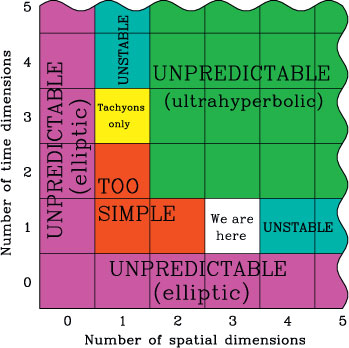
|
‘Martin Rees proposes that the dimensionality of the universe is one of six parameters that appear particularly adjusted to enable life …Clearly Rees regards the dimensionality of space as a property of objective reality. But is it? I think not. Since the space-time model is a human invention, so must be the dimensionality of space-time. We choose it to be three because it fits the data. In the string model, we choose it to be ten. We use whatever works, but that does not mean that reality is exactly that way.’ (Foft 51)
In response, we do not need to think of dimensionality as a property of objective reality. We just rephrase the claim: instead of ‘if space were not three dimensional, then life would not exist’, we instead claim ‘if whatever exists were not such that it is accurately described on macroscopic scales by a model with three space dimensions, then life would not exist’. This (admittedly inelegant sentence) makes no claims about the universe being really three-dimensional. If ‘whatever works’ was four dimensional, then life would not exist, whether the number of dimensions is simply a human invention or an objective fact about the universe. We can still use the dimensionality of space in counterfactual statements about how the universe could have been.
String theory is actually an excellent counterexample to Stenger’s claims. String theorists are not content to posit ten dimensions and leave it at that. They must compactify all but 3+1 of the extra dimensions for the theory to have a chance of describing our universe. This fine-tuning case refers to the number of macroscopic or ‘large’ space dimensions, which both string theory and classical physics agree to be three. The possible existence of small, compact dimensions is irrelevant.
Finally, Stenger tells us (Foft 48) that ‘when a model has passed many risky tests …we can begin to have confidence that it is telling us something about the real world with certainty approaching 100 percent’. One wonders how the idea that space has three (large) dimensions fails to meet this criterion. Stenger’s worry seems to be that the three-dimensionality of space may not be a fundamental property of our universe, but rather an emergent one. Our model of space as a subset of33  may crumble into spacetime foam below the Planck length. But emergent does not imply subjective. Whatever the fundamental properties of spacetime are, it is an objective fact about physical reality — by Stenger’s own criterion — that in the appropriate limit space is accurately modelled by
  .
.
The confusion of Stenger’s response is manifest in the sentence: ‘We choose three [dimensions] because it fits the data’ (Foft 51). This isn’t much of a choice. One is reminded of the man who, when asked why he choose to join the line for ‘non-hen-pecked husbands’, answered, ‘because my wife told me to’. The universe will let you choose, for example, your unit of length. But you cannot decide that the macroscopic world has four space dimensions. It is a mathematical fact that in a universe with four spatial dimensions you could, with a judicious choice of axis, make a left-footed shoe into a right-footed one by rotating it. Our inability to perform such a transformation is not the result of physicists arbitrarily deciding that, in this spacetime model we’re inventing, space will have three dimensions.
5 The Multiverse
On Boxing Day, 2002, Powerball announced that Andrew J. Whittaker Jr. of West Virginia had won $314.9 million in their lottery. The odds of this event are 1 in 120 526 770. How could such an unlikely event occur? Should we accuse Mr Whittaker of cheating? Probably not, because a more likely explanation is that a great many different tickets were sold, increasing the chances that someone would win.
The multiverse is just such an explanation. Perhaps there are more universes out there (in some sense), sufficiently numerous and varied that it is not too improbable that at least one of them would be in the life-permitting subset of possible-physics-space. And, just as Powerball wouldn’t announce that ‘Joe Smith of Chicago didn’t win the lottery today’, so there is no one in the life-prohibiting universes to wonder what went wrong.
Stenger says (Foft 24) that he will not need to appeal to a multiverse in order to explain fine-tuning. He does, however, keep the multiverse close in case of emergencies.
‘Cosmologists have proposed a very simple solution to the fine-tuning problem. Their current models strongly suggest that ours is not the only universe but part of a multiverse containing an unlimited number of individual universes extending an unlimited distance in all directions and for an unlimited time in the past and future. …Modern cosmological theories do indicate that ours is just one of an unlimited number of universes, and theists can give no reason for ruling them out.’ (Foft 22,42)
Firstly, the difficulty in ruling out multiverses speaks to their unfalsifiability, rather than their steadfastness in the face of cosmological data. There is very little evidence, one way or the other. Moreover, there are plenty of reasons given in the scientific literature to be skeptical of the existence of a multiverse. Even their most enthusiastic advocate isn’t as certain about the existence of a multiverse as Stenger suggests.
A multiverse is not part of nor a prediction of the concordance model of cosmology. It is the existence of small, adiabatic, nearly-scale invariant, Gaussian fluctuations in a very-nearly-flat FLRW model (containing dark energy, dark matter, baryons and radiation) that is strongly suggested by the data. Inflation is one idea of how to explain this data. Some theories of inflation, such as chaotic inflation, predict that some of the properties of universes vary from place to place. Carr & Ellis (2008) write:
[Ellis:] A multiverse is implied by some forms of inflation but not others. Inflation is not yet a well defined theory and chaotic inflation is just one variant of it. …the key physics involved in chaotic inflation (Coleman-de Luccia tunnelling) is extrapolated from known and tested physics to quite different regimes; that extrapolation is unverified and indeed unverifiable. The physics is hypothetical rather than tested. We are being told that what we have is ‘known physics → multiverse’. But the real situation is ‘known physics → hypothetical physics → multiverse’ and the first step involves a major extrapolation which may or may not be correct.
Stenger fails to distinguish between the concordance model of cosmology, which has excellent empirical support but in no way predicts a multiverse, and speculative models of the early universe, only some of which predict a multiverse, all of which rely on hypothetical physics, and none of which have unambiguous empirical support, if any at all.
5.1 How to Make A Multiverse
What does it take to specify a multiverse? Following Ellis, Kirchner & Stoeger (2004), we need to:
-
Determine the set of possible universes
 .
. -
Characterise each universe in
 by a set
  of distinguishing parameters p, being careful to create equivalence classes of physically identical universes with different p. The parameters p will need to specify the laws of nature, the parameters of those laws and the particular solution to those laws that describes the given member m of
  , which usually involves initial or boundary conditions.
 -
Propose a distribution function f(m) on
 , specifying how many times each possible universe m is realised. Note that simply saying that all possibilities exist only tells us that f(m) > 0 for all m in
  . It does not specify f(m).
 -
Define a distribution function over continuous parameters, relative to a measure π, which assigns a probability space volume to each parameter increment.
We would also like to know the set of universes which allow the existence of conscious observers — the anthropic subset.
As Ellis et al. (2004) point out, any such proposal will have to deal with the problems of what determines { }, actualized infinities (in
  , f(m) and the spatial extent of universes) and non-renormalisability, the parameter dependence and non-uniqueness of π, and how one could possibly observationally confirm any of these quantities. If some meta-law is proposed to physically generate a multiverse, then we need to postulate not just a.) that the meta-law holds in this universe, but b.) that it holds in some pre-existing metaspace beyond our universe. There is no unambiguous evidence in favour of a.) for any multiverse, and b.) will surely forever hold the title of the most extreme extrapolation in all of science, if indeed it can be counted as part of science. We turn to this topic now.
5.2 Is it Science?
Could a multiverse proposal ever be regarded as scientific? Foft 228 notes the similarity between undetectable universes and undetectable quarks, but the analogy is not a good one. The properties of quarks — mass, charge, spin, etc. — can be inferred from measurements. Quarks have a causal effect on particle accelerator measurements; if the quark model were wrong, we would know about it. In contrast, we cannot observe any of the properties of a multiverse { }, as they have no causal effect on our universe. We could be completely wrong about everything we believe about these other universes and no observation could correct us. The information is not here. The history of science has repeatedly taught us that experimental testing is not an optional extra. The hypothesis that a multiverse actually exists will always be untestable.
The most optimistic scenario is where a physical theory, which has been well-tested in our universe, predicts a universe-generating mechanism. Even then, there would still be questions beyond the reach of observation, such as whether the necessary initial conditions for the generator hold in the metaspace, and whether there are modifications to the physical theory that arise at energy scales or on length scales relevant to the multiverse but beyond testing in our universe. Moreover, the process by which a new universe is spawned almost certainly cannot be observed.
5.3 The Principle of Mediocrity
One way of testing a particular multiverse proposal is the so-called principle of mediocrity. This is a self-consistency test — it cannot pick out a unique multiverse as the ‘real’ multiverse — but can be quite powerful. We will present the principle using an illustration. Boltzmann (1895), having discussed the discovery that the second law of thermodynamics is statistical in nature, asks why the universe is currently so far from thermal equilibrium. Perhaps, Boltzmann says, the universe as a whole is in thermal equilibrium. From time to time, however, a random statistical fluctuation will produce a region which is far from equilibrium. Since life requires low entropy, it could only form in such regions. Thus, a randomly chosen region of the universe would almost certainly be in thermal equilibrium. But if one were to take a survey of all the intelligent life in such a universe, one would find them all scratching their heads at the surprisingly low entropy of their surroundings.
It is a brilliant idea, and yet something is wrong34. At most, life only needs a low entropy fluctuation a few tens of Mpc in size — cosmological structure simulations show that the rest of the universe has had virtually no effect on galaxy/star/planet/life formation where we are. And yet, we find ourselves in a low entropy region that is tens of thousands of Mpc in size, as far as our telescopes can see.
Why is this a problem? Because the probability of a thermal fluctuation decreases exponentially with its volume. This means that a random observer is overwhelmingly likely to observe that they are in the smallest fluctuation able to support an observer. If one were to take a survey of all the life in the multiverse, an incredibly small fraction would observe that they are inside a fluctuation whose volume is at least a billion times larger than their existence requires. In fact, our survey would find vastly many more observers who were simply isolated brains that fluctuated into existence preloaded with false thoughts about being in a large fluctuation. It is more likely that we are wrong about the size of the universe, that the distant galaxies are just a mirage on the face of the thermal equilibrium around us. The Boltzmann multiverse is thus definitively ruled out.
5.4 Coolness and the Measure Problem
Do more modern multiverse proposals escape the mediocrity test? Tegmark (2005) discusses what is known as the coolness problem, also known as the youngness paradox. Suppose that inflation is eternal, in the sense (Guth 2007) the universe is always a mix of inflating and non-inflating regions. In our universe, inflation ended 13.7 billion years ago and a period of matter-dominated, decelerating expansion began. Meanwhile, other regions continued to inflate. Let’s freeze the whole multiverse now, and take our survey clipboard around to all parts of the multiverse. In the regions that are still inflating, there is almost no matter and so no life. So we need to look for life in the parts that have stopped inflating. Whenever we find an intelligent life form, we’ll ask how long ago their part of the universe stopped inflating. Since the temperature of a post-inflation region is at its highest just as inflation ends and drops as the universe expands, we could equivalently ask: what is the temperature of the CMB in your universe?
The results of this survey would be rather surprising: an extremely small fraction of life-permitting universes are as old and cold as ours. Why? Because other parts of the universe continued to inflate after ours had stopped. These regions become exponentially larger, and thus nucleate exponentially more matter-dominated regions, all of which are slightly younger and warmer than ours. There are two effects here: there are many more younger universes, but they will have had less time to make intelligent life. Which effect wins? Are there more intelligent observers who formed early in younger universes or later in older universes? It turns out that the exponential expansion of inflation wins rather comfortably. For every observer in a universe as old as ours, there are 101038 observers who live in a universe that is one second younger. The probability of observing a universe with a CMB temperature of 2.75 K or less is approximately 1 in 101056.
Alas! Is this the end of the inflationary multiverse as we know it? Not necessarily. The catch comes in the seemingly innocent word now. We are considering the multiverse at a particular time. But general relativity will not allow it — there is no unique way to specify ‘now’. We can’t just compare our universe with all the other universes in existence ‘now’. But we must be able to compare the properties of our universe with some subset of the multiverse — otherwise the multiverse proposal cannot make predictions. This is the ‘measure problem’ of cosmology, on which there is an extensive literature — Page (2011a) lists 70 scientific papers. As Linde & Noorbala (2010) explains, one of the main problems is that ‘in an eternally inflating universe the total volume occupied by all, even absolutely rare types of the ‘universes’, is indefinitely large’. We are thus faced with comparing infinities. In fact, even if inflation is not eternal and the universe is finite, the measure problem can still paralyse our analysis.
The moral of the coolness problem is not that the inflationary multiverse has been falsified. Rather, it is this: no measure, no nothing. For a multiverse proposal to make predictions, it must be able to calculate and justify a measure over the set of universes it creates. The predictions of the inflationary multiverse are very sensitive to the measure, and thus in the absence of a measure, we cannot conclude that it survives the test of the principle of mediocrity.
5.5 Our Island in the Multiverse
A closer look at our island in parameter space reveals a refinement of the mediocrity test, as discussed by Aguirre (2007); see also Bousso, Hall & Nomura (2009). It is called the ‘principle of living dangerously’: if the prior probability for a parameter is a rapidly increasing (or decreasing) function, then we expect the observed value of the parameter to lie near the edge of the anthropically allowed range. One particular parameter for which this could be a problem is Q, as discussed in Section 4.5. Fixing other cosmological parameters, the anthropically allowed range is 10–6 ![]() Q
Q ![]() 10–4. The observed value (~10–5) isn’t close to either edge of the anthropic range. This creates problems for inflationary multiverses, which are either fine-tuned to have the prior for Q to peak near the observed value, or else are steep functions of Q in the anthropic range (Graesser et al. 2004; Feldstein, Hall & Watari 2005).
10–4. The observed value (~10–5) isn’t close to either edge of the anthropic range. This creates problems for inflationary multiverses, which are either fine-tuned to have the prior for Q to peak near the observed value, or else are steep functions of Q in the anthropic range (Graesser et al. 2004; Feldstein, Hall & Watari 2005).
The discovery of another life-permitting island in parameter space potentially creates a problem for the multiverse. If the other island is significantly larger than ours (for a given multiverse measure), then observers should expect to be on the other island. An example is the cold big bang, as described by Aguirre (2001). Aguirre’s aim in the paper is to provide a counterexample to what he calls the anthropic program: ‘the computation of P [the probability that a randomly chosen observer measures a given set of cosmological parameters]; if this probability distribution has a single peak at a set [of parameters] and if these are near the measured values, then it could be claimed that the anthropic program has ‘explained’ the values of the parameters of our cosmology’. Aguirre’s concern is a lack of uniqueness.
The cold big bang (CBB) is a model of the universe in which the (primordial) ratio of photons to baryons is ηγ ~ 1. To be a serious contender as a model of our universe (in which ηγ ~ 109) there would need to be an early population of luminous objects e.g. PopIII stars. Nucleosynthesis generally proceeds further than in our universe, creating an approximately solar metalicity intergalactic medium along with a 25% helium mass fraction35. Structure formation is not suppressed by CMB radiation pressure, and thus stars and galaxies require a smaller value of Q.
How much of a problem is the cold big bang to a multiverse explanation of cosmological parameters? Particles and antiparticles pair off and mutually annihilate to photons as the universe cools, so the excess of particles over antiparticles determines the value of ηγ. We are thus again faced with the absence of a successful theory of baryogenesis and leptogenesis. It could be that small values of ηγ, which correspond to larger baryon and lepton asymmetry, are very rare in the multiverse. Nevertheless, the conclusion of Aguirre (2001) seems sound: ‘[the CBB] should be discouraging for proponents of the anthropic program: it implies that it is quite important to know the [prior] probabilities P, which depend on poorly constrained models of the early universe’.
Does the cold big bang imply that cosmology need not be fine-tuned to be life-permitting? Aguirre (2001) claims that ξ(ηγ ~ 1, 10–11 < Q < 10–5) ~ ξ(ηγ ~ 109, 10–6 <Q < 10–4), where ξ is the number of solar mass stars per baryon. At best, this would show that there is a continuous life-permitting region, stretching along the ηγ axis. Various compensating factors are needed along the way — we need a smaller value of Q, which renders atomic cooling inefficient, so we must rely on molecular cooling, which requires higher densities and metalicities, but not too high or planetary orbits will be disrupted collisions (whose frequency increases as ηγ–4Q7/2). Aguirre (2001) only considers the case ηγ ~ 1 in detail, so it is not clear whether the CBB island connects to the HBB island (106 ![]() ηγ
ηγ ![]() 1011) investigated by Tegmark & Rees (1998). Either way, life does not have free run of parameter space.
1011) investigated by Tegmark & Rees (1998). Either way, life does not have free run of parameter space.
5.6 Boltzmann’s Revenge
The spectre of the demise of Boltzmann’s multiverse haunts more modern cosmologies in two different ways. The first is the possibility of Boltzmann brains. We should be wary of any multiverse which allows for single brains, imprinted with memories, to fluctuate into existence. The worry is that, for every observer who really is a carbon-based life form who evolved on a planet orbiting a star in a galaxy, there are vastly more for whom this is all a passing dream, the few, fleeting fancies of a phantom fluctuation. This could be a problem in our universe — if the current, accelerating phase of the universe persists arbitrarily into the future, then our universe will become vacuum dominated. Observers like us will die out, and eventually Boltzmann brains, dreaming that they are us, will outnumber us. The most serious problem is that, unlike biologically evolved life like ourselves, Boltzmann brains do not require a fine-tuned universe. If we condition on observers, rather than biological evolved life, then the multiverse may fail to predict a universe like ours. The multiverse would not explain why our universe is fine-tuned for biological life (R. Collins, forthcoming).
Another argument against the multiverse is given by Penrose (2004, p. 763ff). As with the Boltzmann multiverse, the problem is that this universe seems uncomfortably roomy.
‘…do we really need the whole observable universe, in order that sentient life can come about? This seems unlikely. It is hard to imagine that even anything outside our galaxy would be needed …Let us be very generous and ask that a region of radius one tenth of the …observable universe must resemble the universe that we know, but we do not care about what happens outside that radius …Assuming that inflation acts in the same way on the small region [that inflated into the one-tenth smaller universe] as it would on the somewhat larger one [that inflated into ours], but producing a smaller inflated universe, in proportion, we can estimate how much more frequently the Creator comes across the smaller than the larger regions. The figure is no better than 1010123. You see what an incredible extravagance it was (in terms of probability) for the Creator to bother to produce this extra distant part of the universe, that we don’t actually need …for our existence.’
In other words, if we live in a multiverse generated by a process like chaotic inflation, then for every observer who observes a universe of our size, there are 1010123 who observe a universe that is just 10 times smaller. This particular multiverse dies the same death as the Boltzmann multiverse. Penrose’s argument is based on the place of our universe in phase space, and is thus generic enough to apply to any multiverse proposal that creates more small universe domains than large ones. Most multiverse mechanisms seem to fall into this category.
5.7 Conclusion
A multiverse generated by a simple underlying mechanism is a remarkably seductive idea. The mechanism would be an extrapolation of known physics, that is, physics with an impressive record of explaining observations from our universe. The extrapolation would be natural, almost inevitable. The universe as we know it would be a very small part of a much larger whole. Cosmology would explore the possibilities of particle physics; what we know as particle physics would be mere by-laws in an unimaginably vast and variegated cosmos. The multiverse would predict what we expect to observe by predicting what conditions hold in universes able to support observers.
Sadly, most of this scenario is still hypothetical. The goal of this section has been to demonstrate the mountain that the multiverse is yet to climb, the challenges that it must face openly and honestly. The multiverse may yet solve the fine-tuning of the universe for intelligent life, but it will not be an easy solution. ‘Multiverse’ is not a magic word that will make all the fine-tuning go away. For a popular discussion of these issues, see Ellis (2011).
6 Conclusions and Future
We conclude that the universe is fine-tuned for the existence of life. Of all the ways that the laws of nature, constants of physics and initial conditions of the universe could have been, only a very small subset permits the existence of intelligent life.
Will future progress in fundamental physics solve the problem of the fine-tuning of the universe for intelligent life, without the need for a multiverse? There are a few ways that this could happen. We could discover that the set of life-permitting universes is much larger than previously thought. This is unlikely, since the physics relevant to life is low-energy physics, and thus well-understood. Physics at the Planck scale will not rewrite the standard model of particle physics. It is sometimes objected that we do not have an adequate definition of ‘an observer’, and we do not know all possible forms of life. This is reason for caution, but not a fatal flaw of fine-tuning. If the strong force were weaker, the periodic table would consist of only hydrogen. We do not need a rigorous definition of life to reasonably conclude that a universe with one chemical reaction (2H → H2) would not be able to create and sustain the complexity necessary for life.
Alternatively, we could discover that the set of possible universes is much smaller than we thought. This scenario is much more interesting. What if, when we really understand the laws of nature, we will realise that they could not have been different? We must be clear about the claim being made. If the claim is that the laws of nature are fixed by logical and mathematical necessity, then this is demonstrably wrong — theoretical physicists find it rather easy to describe alternative universes that are free from logical contradiction (Davies, in Davies 2003). The category of ‘physically possible’ isn’t much help either, as the laws of nature tell us what is physically possible, but not which laws are possible.
It is not true that fine-tuning must eventually yield to the relentless march of science. Fine-tuning is not a typical scientific problem, that is, a phenomenon in our universe that cannot be explained by our current understanding of physical laws. It is not a gap. Rather, we are concerned with the physical laws themselves. In particular, the anthropic coincidences are not like, say, the coincidence between inertial mass and gravitational mass in Newtonian gravity, which is a coincidence between two seemingly independent physical quantities. Anthropic coincidences, on the other hand, involve a happy consonance between a physical quantity and the requirements of complex, embodied intelligent life. The anthropic coincidences are so arresting because we are accustomed to thinking of physical laws and initial conditions as being unconcerned with how things turn out. Physical laws are material and efficient causes, not final causes. There is, then, no reason to think that future progress in physics will render a life-permitting universe inevitable. When physics is finished, when the equation is written on the blackboard and fundamental physics has gone as deep as it can go, fine-tuning may remain, basic and irreducible.
Perhaps the most optimistic scenario is that we will eventually discover a simple, beautiful physical principle from which we can derive a unique physical theory, whose unique solution describes the universe as we know it, including the standard model, quantum gravity, and (dare we hope) the initial conditions of cosmology. While this has been the dream of physicists for centuries, there is not the slightest bit of evidence that this idea is true. It is almost certainly not true of our best hope for a theory of quantum gravity, string theory, which has ‘anthropic principle written all over it’ (Schellekens 2008). The beauty of its principles has not saved us from the complexity and contingency of the solutions to its equations. Beauty and simplicity are not necessity.
Finally, it would be the ultimate anthropic coincidence if beauty and complexity in the mathematical principles of the fundamental theory of physics produced all the necessary low-energy conditions for intelligent life. This point has been made by a number of authors, e.g. Carr & Rees (1979) and Aguirre (2005). Here is Wilczek (2006b):
‘It is logically possible that parameters determined uniquely by abstract theoretical principles just happen to exhibit all the apparent fine-tunings required to produce, by a lucky coincidence, a universe containing complex structures. But that, I think, really strains credulity.’
References
Adams, F. C., 2008, JCAP, 2008, 010Agrawal, V., Barr, S. M., Donoghue, J. F. and Seckel, D., 1998a, PhRvL, 80, 1822
| 1:CAS:528:DyaK1cXhsFSgtb4%3D&md5=327084b8088628bcf8e9263f7429b32dCAS |
Agrawal, V., Barr, S. M., Donoghue, J. F. and Seckel, D., 1998b, PhRvD, 57, 5480
| 1:CAS:528:DyaK1cXisVeht7c%3D&md5=9079f66a6d59f571cf5a16855020fd79CAS |
Aguirre, A., 1999, ApJ, 521, 17
| Crossref | GoogleScholarGoogle Scholar | 1:CAS:528:DyaK1MXlsFWnu70%3D&md5=1e395825da456aa0a9620f298182ba9bCAS |
Aguirre, A., 2001, PhRvD, 64, 083508
Aguirre, A., 2005, ArXiv:astro-ph/0506519
Aguirre, A., 2007, in Universe or Multiverse?, ed. B. J. Carr (Cambridge: Cambridge University Press), 367
Aitchison, I. & Hey, A., 2002, Gauge Theories in Particle Physics: Volume 1 — From Relativistic Quantum Mechanics to QED (3rd edition; New York: Taylor & Francis)
Arkani-Hamed, N. and Dimopoulos, S., 2005, JHEP, 2005, 073
Arkani-Hamed, N., Dimopoulos, S. & Kachru, S., 2005, ArXiv: hep-th/0501082
Barnes, L. A., Francis, M. J., Lewis, G. F. and Linder, E. V., 2005, PASA, 22, 315
| Crossref | GoogleScholarGoogle Scholar |
Barr, S. M. and Khan, A., 2007, PhRvD, 76, 045002
Barrow, J. D. & Tipler, F. J., 1986, The Anthropic Cosmological Principle (Oxford: Clarendon Press)
Bekenstein, J. D., 1973, PhRvD, 7, 2333
Boltzmann, L., 1895, Natur, 51, 413
| Crossref | GoogleScholarGoogle Scholar |
Bousso, R., 2008, GReGr, 40, 607
Bousso, R. and Leichenauer, S., 2009, PhRvD, 79, 063506
Bousso, R. and Leichenauer, S., 2010, PhRvD, 81, 063524
Bousso, R., Hall, L. and Nomura, Y., 2009, PhRvD, 80, 063510
Bradford, R. A. W., 2009, JApA, 30, 119
| 1:CAS:528:DC%2BD1MXhtFCkt7fK&md5=c7b1c4ae02432bd9e407ec4644827fb5CAS |
Brandenberger, R. H., 2011, ArXiv:astro-ph/1103.2271
Burgess, C. & Moore, G., 2006, The Standard Model: A Primer (Cambridge: Cambridge University Press)
Cahn, R., 1996, RvMP, 68, 951
| 1:CAS:528:DyaK28XlvFart78%3D&md5=a79883dbfcffdfd9e0ed02147d5f8e4aCAS |
Carr, B. J. and Ellis, G. F. R., 2008, A&G, 49, 2.29
| 1:CAS:528:DC%2BD1cXltlKksbk%3D&md5=e19d773c2383af556987fa8afaf802b7CAS |
Carr, B. J. and Rees, M. J., 1979, Natur, 278, 605
| Crossref | GoogleScholarGoogle Scholar |
Carroll, S. M., 2001, LRR, 4, 1
Carroll, S. M., 2003, Spacetime and Geometry: An Introduction to General Relativity (San Francisco: Benjamin Cummings)
Carroll, S. M., 2008, SciAm, 298, 48
| 1:CAS:528:DC%2BD1cXnsVSisL8%3D&md5=7cc80f07b33fdf90848e04b84f71f19eCAS |
Carroll, S. M. & Tam, H., 2010, ArXiv:astro-ph/1007.1417
Carter, B., 1974, in IAU Symposium, Vol. 63, Confrontation of Cosmological Theories with Observational Data, ed. M. S. Longair (Boston: D. Reidel Pub. Co.), 291
Clavelli, L. & White, R. E., 2006, ArXiv:hep-ph/0609050
Cohen, B. L., 2008, PhTea, 46, 285
Collins, R., 2003, in The Teleological Argument and Modern Science, ed. N. Manson (London: Routledge), 178
Csótó, A., Oberhummer, H. and Schlattl, H., 2001, NuPhA, 688, 560
Damour, T. and Donoghue, J. F., 2008, PhRvD, 78, 014014
Davies, P. C. W., 1972, JPhA, 5, 1296
| 1:CAS:528:DyaE38XkvVahurw%3D&md5=4ece752ea00470a3d5eaf1e0bbb462e3CAS |
Davies, P., 2003, in God and Design: The Teleological Argument and Modern Science, ed. N. A. Manson (London: Routledge), 147
Davies, P. C. W., 2006, The Goldilocks Enigma: Why is the Universe Just Right for Life? (London: Allen Lane)
Davies, C. et al., 2004, PhRvL, 92,
| 1:CAS:528:DC%2BD2cXkvFKjsg%3D%3D&md5=f8fb9835f6a2f9dcbaf8cb89ea48062cCAS |
Dawkins, R., 1986, The Blind Watchmaker (New York: W. W. Norton & Company)
Dawkins, R., 2006, The God Delusion (New York: Houghton Mifflin Harcourt)
De Boer, W., 1994, PrPNP, 33, 201
| 1:CAS:528:DyaK2cXms1Gjs7o%3D&md5=980c8ba0d6064595c59d93eda8cf8c02CAS |
De Boer, W. and Sander, C., 2004, PhLB, 585, 276
| 1:CAS:528:DC%2BD2cXitlGqur0%3D&md5=ffa154aec3672ff57ba918b6d10923afCAS |
Donoghue, J. F., 2007, in Universe or Multiverse?, ed. B. J. Carr (Cambridge: Cambridge University Press), 231
Donoghue, J. F., Dutta, K., Ross, A. and Tegmark, M., 2010, PhRvD, 81,
Dorling, J., 1970, AmJPh, 38, 539
Dürr, S. et al., 2008, Sci, 322, 1224
| Crossref | GoogleScholarGoogle Scholar |
Durrer, R. and Maartens, R., 2007, GReGr, 40, 301
Dyson, F. J., 1971, SciAm, 225, 51
Earman, J., 2003, in Symmetries in Physics: Philosophical Reflections, ed. K. Brading & E. Castellani (Cambridge: Cambridge University Press), 140
Ehrenfest, P., 1917, Proc. Amsterdam Academy, 20, 200
Ekström, S., Coc, A., Descouvemont, P., Meynet, G., Olive, K. A., Uzan, J.-P. and Vangioni, E., 2010, A&A, 514, A62
Ellis, G. F. R., 1993, in The Anthropic Principle, ed. F. Bertola & U. Curi (Oxford: Oxford University Press), 27
Ellis, G. F. R., 2011, SciAm, 305, 38
Ellis, G. F. R., Kirchner, U. and Stoeger, W. R., 2004, MNRAS, 347, 921
| Crossref | GoogleScholarGoogle Scholar | 1:CAS:528:DC%2BD2cXhsVGisrc%3D&md5=5b08b4a3c24154a51ad584f9b038517dCAS |
Feldstein, B., Hall, L. and Watari, T., 2005, PhRvD, 72, 123506
Feldstein, B., Hall, L. and Watari, T., 2006, PhRvD, 74, 095011
Freeman, I. M., 1969, AmJPh, 37, 1222
Garriga, J. and Vilenkin, A., 2006, PThPS, 163, 245
Garriga, J., Livio, M. and Vilenkin, A., 1999, PhRvD, 61, 023503
Gasser, J. and Leutwyler, H., 1982, PhR, 87, 77
| 1:CAS:528:DyaL38XlsFWktrk%3D&md5=950f74b616f9ba2e67e16844edeaac1dCAS |
Gedalia, O., Jenkins, A. and Perez, G., 2011, PhRvD, 83,
| 1:CAS:528:DC%2BC3MXps1Siu7c%3D&md5=83ab5eb378b1b99f3df17bee7659faa3CAS |
Gibbons, G. W. and Turok, N., 2008, PhRvD, 77, 063516
Gibbons, G. W., Hawking, S. W. and Stewart, J. M., 1987, NuPhB, 281, 736
Gingerich, O., 2008, in Fitness of the Cosmos for Life: Biochemistry and Fine-Tuning, ed. J. D. Barrow, S. C. Morris, S. J. Freeland & C. L. Harper (Cambridge: Cambridge University Press), 20
Gould, A., 2010, ArXiv:hep-ph/1011.2761
Graesser, M. L., Hsu, S. D. H., Jenkins, A. and Wise, M. B., 2004, PhLB, 600, 15
| 1:CAS:528:DC%2BD2cXnvVKgu74%3D&md5=07345d4317ca55f1b9100fa3a45a7382CAS |
Greene, B., 2011, The Hidden Reality: Parallel Universes and the Deep Laws of the Cosmos (New York: Knopf)
Griffiths, D. J., 2008, Introduction to Elementary Particles (Weinheim: Wiley-VCH)
Gurevich, L., 1971, PhLA, 35, 201
Guth, A. H., 1981, PhRvD, 23, 347
| 1:CAS:528:DyaL3MXnt1yluw%3D%3D&md5=4cd171656e215b03a58fcc7b39e45bd9CAS |
Guth, A. H., 2007, JPhA, 40, 6811
Hall, L. and Nomura, Y., 2008, PhRvD, 78, 035001
Hall, L. and Nomura, Y., 2010, JHEP, 2010, 76
Harnik, R., Kribs, G. and Perez, G., 2006, PhRvD, 74, 035006
Harrison, E. R., 1970, PhRvD, 1, 2726
Harrison, E. R., 2003, Masks of the Universe (2nd edition; Cambridge: Cambridge University Press)
Hartle, J. B., 2003, Gravity: An Introduction to Einstein's General Relativity (San Francisco: Addison Wesley)
Hawking, S. W., 1975, CMaPh, 43, 199
Hawking, S. W., 1988, A Brief History of Time (Toronto: Bantam)
Hawking, S. W. & Mlodinow L., 2010, The Grand Design (Toronto: Bantam)
Hawking, S. W. and Page, D. N., 1988, NuPhB, 298, 789
Healey, R., 2007, Gauging What's Real: The Conceptual Foundations of Gauge Theories (New York: Oxford University Press)
Hogan, C. J., 2000, RvMP, 72, 1149
| 1:CAS:528:DC%2BD3cXovVGrsbw%3D&md5=9cbf31c00b1e2ca522112d2dca41e9c8CAS |
Hogan, C. J., 2006, PhRvD, 74, 123514
Hogan, C. J., 2007, in Universe or Multiverse?, ed. B. J. Carr (Cambridge: Cambridge University Press), 221
Hollands, S. & Wald, R. M., 2002a, ArXiv:hep-th/0210001
Hollands, S. and Wald, R. M., 2002b, GReGr, 34, 2043
Iwasaki, Y., 2000, PThPS, 138, 1
| 1:CAS:528:DC%2BD3cXjs1Wrsrk%3D&md5=5564958c5eb3d20af2a9ac5799fd15c7CAS |
Jaffe, R., Jenkins, A. and Kimchi, I., 2009, PhRvD, 79, 065014
Jeltema, T. and Sher, M., 1999, PhRvD, 61, 017301
Kaku, M., 1993, Quantum Field Theory: A Modern Introduction (New York: Oxford University Press)
King, R. A., Siddiqi, A., Allen, W. D. and Schaefer, H. F. I., 2010, PhRvA, 81, 042523
Kofman, L., Linde, A. and Mukhanov, V., 2002, JHEP, 2002, 057
Kostelecký, V. and Russell, N., 2011, RvMP, 83, 11
Laiho, J., 2011, ArXiv:hep-ph/1106.0457
Leslie, J., 1989, Universes (London: Routledge)
Liddle, A., 1995, PhRvD, 51, R5347
| 1:CAS:528:DyaK2MXlslOqu7s%3D&md5=7a9505c39163d1c09df235783b987530CAS |
Lieb, E. and Yau, H.-T., 1988, PhRvL, 61, 1695
| 1:CAS:528:DyaL1cXmtlOht7o%3D&md5=dc8c9e852fbe4559e7484f639a3960dbCAS |
Linde, A., 2008, in Lecture Notes in Physics, Vol. 738, Inflationary Cosmology, ed. M. Lemoine, J. Martin & P. Peter (Berlin, Heidelberg: Springer), 1
Linde, A. and Noorbala, M., 2010, JCAP, 2010, 8
Linde, A. & Vanchurin, V., 2010, ArXiv:hep-th/1011.0119
Livio, M., Hollowell, D., Weiss, A. and Truran, J. W., 1989, Natur, 340, 281
| Crossref | GoogleScholarGoogle Scholar | 1:CAS:528:DyaK3cXht1ams7g%3D&md5=1d0c75850c0c52bb6bfc916da32f7a67CAS |
Lynden-Bell, D., 1969, Natur, 223, 690
| Crossref | GoogleScholarGoogle Scholar |
MacDonald, J. and Mullan, D. J., 2009, PhRvD, 80, 043507
Martin, S. P., 1998, in Perspectives on Supersymmetry, ed. G. L. Kane (Singapore: World Scientific Publishing), 1
Martin, C. A., 2003, in Symmetries in Physics: Philosophical Reflections, ed. K. Brading & E. Castellani (Cambridge: Cambridge University Press), 29
Misner, C. W., Thorne, K. S. & Wheeler, J. A., 1973, Gravitation (San Francisco: W. H. Freeman and Co)
Mo, H., van den Bosch, F. C. & White, S. D. M., 2010, Galaxy Formation and Evolution (Cambridge: Cambridge University Press)
Nagashima, Y., 2010, Elementary Particle Physics: Volume 1: Quantum Field Theory and Particles (Wiley-VCH)
Nakamura, K., 2010, JPhG, 37, 075021
Norton, J. D., 1995, Erkenntnis, 42, 223
| Crossref | GoogleScholarGoogle Scholar |
Oberhummer, H., 2001, NuPhA, 689, 269
Oberhummer, H., Pichler, R. & Csótó, A., 1998, ArXiv:nuclth/9810057
Oberhummer, H., Csótó, A. & Schlattl, H., 2000a, in The Future of the Universe and the Future of Our Civilization, ed. V. Burdyuzha & G. Khozin (Singapore: World Scientific Publishing), 197
Oberhummer, H., Csótó, A. and Schlattl, H., 2000b, Sci, 289, 88
| Crossref | GoogleScholarGoogle Scholar | 1:CAS:528:DC%2BD3cXlt1enu7s%3D&md5=4f9e201e7eadda4e7086802298151b7eCAS |
Padmanabhan, T., 2007, GReGr, 40, 529
Page, D. N., 2011a, JCAP, 2011, 031
Page, D. N., 2011b, ArXiv e-prints: 1101.2444
Peacock, J. A., 1999, Cosmological Physics (Cambridge: Cambridge University Press)
Peacock, J. A., 2007, MNRAS, 379, 1067
| Crossref | GoogleScholarGoogle Scholar |
Penrose, R., 1959, MPCPS, 55, 137
Penrose, R., 1979, in General Relativity: An Einstein Centenary Survey, ed. S. W. Hawking & W. Israel (Cambridge: Cambridge University Press), 581
Penrose, R., 1989, NYASA, 571, 249
| Crossref | GoogleScholarGoogle Scholar | 1:CAS:528:DyaK3MXht12ktA%3D%3D&md5=4dac3974c0d97c2f1a627b63e8588751CAS |
Penrose, R., 2004, The Road to Reality: A Complete Guide to the Laws of the Universe (London: Vintage)
Phillips, A. C., 1999, The Physics of Stars (2nd edition; Chichester: Wiley)
Pogosian, L. and Vilenkin, A., 2007, JCAP, 2007, 025
Pokorski, S., 2000, Gauge Field Theories (Cambridge: Cambridge University Press)
Polchinski, J., 2006, ArXiv:hep-th/0603249
Polkinghorne, J. C. & Beale, N., 2009, Questions of Truth: Fifty-One Responses to Questions about God, Science, and Belief (Louisville: Westminster John Knox Press)
Pospelov, M. and Romalis, M., 2004, PhT, 57, 40
| 1:CAS:528:DC%2BD2cXmt1yls74%3D&md5=baae41b63e2acd999b886f5d4e4313bcCAS |
Price, H., 1997, in Time's Arrows Today: Recent Physical and Philosophical Work on the Direction of Time, ed. S. F. Savitt (Cambridge: Cambridge University Press), 66
Price, H., 2006, Time and Matter – Proceedings of the International Colloquium on the Science of Time, ed. I. I. Bigi (Singapore: World Scientific Publishing), 209
Redfern, M., 2006, The Anthropic Universe, ABC Radio National, available at http://www.abc.net.au/rn/scienceshow/stories/2006/1572643.htm
Rees, M. J., 1999, Just Six Numbers: The Deep Forces that Shape the Universe (New York: Basic Books)
Sakharov, A. D., 1967, JETPL, 5, 24
Schellekens, A. N., 2008, RPPh, 71, 072201
Schlattl, H., Heger, A., Oberhummer, H., Rauscher, T. and Csótó, A., 2004, ApSS, 291, 27
| 1:CAS:528:DC%2BD2cXksFShsbY%3D&md5=3ddca43502c641a6a754d767444af3c2CAS |
Schmidt, M., 1963, Natur, 197, 1040
| Crossref | GoogleScholarGoogle Scholar |
Schrödinger, E., 1992, What Is Life? (Cambridge: Cambridge University Press)
Shaw, D. and Barrow, J. D., 2011, PhRvD, 83,
Smolin, L., 2007, in Universe or Multiverse?, ed. B. Carr (Cambridge: Cambridge University Press), 323
Steinhardt, P. J., 2011, SciAm, 304, 36
Strocchi, F., 2007, Symmetry Breaking (Berlin, Heidelberg: Springer)
Susskind, L., 2003, ArXiv:hep-th/0302219
Susskind, L., 2005, The Cosmic Landscape: String Theory and the Illusion of Intelligent Design (New York: Little, Brown and Company)
Taubes, G., 2002, Interview with Lisa Randall, ESI Special Topics, available at http://www.esitopics.com/brane/interviews/DrLisaRandall.html
Tegmark, M., 1997, CQGra, 14, L69
| Crossref | GoogleScholarGoogle Scholar | 1:CAS:528:DyaK2sXivV2isLs%3D&md5=d23a1c124b2bb3c46dca27ae3b5f168aCAS |
Tegmark, M., 1998, AnPhy, 270, 1
| 1:CAS:528:DyaK1cXotFahsL0%3D&md5=d0cb6deccb2a46a0b5a97162d9b63ffaCAS |
Tegmark, M., 2005, JCAP, 2005, 001
Tegmark, M. and Rees, M. J., 1998, ApJ, 499, 526
| Crossref | GoogleScholarGoogle Scholar | 1:CAS:528:DyaK1cXktF2mu78%3D&md5=7dfed7bc2984de2f75b1f47f0d50b41bCAS |
Tegmark, M., Vilenkin, A. and Pogosian, L., 2005, PhRvD, 71, 103523
Tegmark, M., Aguirre, A., Rees, M. J. and Wilczek, F., 2006, PhRvD, 73, 023505
Turok, N., 2002, CQGra, 19, 3449
| Crossref | GoogleScholarGoogle Scholar |
Vachaspati, T. and Trodden, M., 1999, PhRvD, 61, 023502
Vilenkin, A., 2003, in Astronomy, Cosmology and Fundamental Physics, ed. P. Shaver, L. Dilella & A. Giméne (Berlin: Springer Verlag), 70
Vilenkin, A., 2006, ArXiv e-prints: hep-th/0610051
Vilenkin, A., 2010, JPhCS, 203, 012001
Weinberg, S., 1989, RvMP, 61, 1
| 1:CAS:528:DyaL1MXht1ejur4%3D&md5=200978d6a99992c73ac7ac2c4bbc6b46CAS |
Weinberg, S., 1994, SciAm, 271, 44
| 1:STN:280:DC%2BD3MnlsFWntg%3D%3D&md5=7c679570dc6910da79195d9d4f1fe963CAS |
Weinberg, S., 2007, in Universe or Multiverse?, ed. B. J. Carr (Cambridge: Cambridge University Press), 29
Wheeler J. A., 1996, At Home in the Universe (New York: AIP Press)
Whitrow, G. J., 1955, BrJPhilosSci, VI, 13
| Crossref | GoogleScholarGoogle Scholar |
Wilczek, F., 1997, in Critical Dialogues in Cosmology, ed. N. Turok (Singapore: World Scientific Publishing), 571
Wilczek, F., 2002, ArXiv:hep-ph/0201222
Wilczek, F., 2005, PhT, 58, 12
Wilczek, F., 2006a, PhT, 59, 10
Wilczek, F., 2006b, PhT, 59, 10
Wilczek, F., 2007, in Universe or Multiverse?, ed. B. J. Carr (Cambridge: Cambridge University Press), 43
Zel'dovich, Y. B., 1964, SPhD, 9, 195
Zel'dovich, Y. B., 1972, MNRAS, 160, 1P
1 We may wish to stipulate that a given observer by definition only observes one universe. Such finer points will not effect our discussion.
2 The counter-argument presented in Stenger’s book (page 252), borrowing from a paper by Ikeda and Jeffreys, does not address this possibility. Rather, it argues against a deity which intervenes to sustain life in this universe. I have discussed this elsewhere: ikedajeff.notlong.com
3 Viz Top Tip: http://www.viz.co.uk/toptips.html
4 Hereafter, ‘Foft x’ will refer to page x of Stenger’s book.
5 References: Barrow & Tipler (1986), Carr & Rees (1979), Carter (1974), Davies (2006), Dawkins (2006), Redfern (2006) for Deutsch’s view on fine-tuning, Ellis (1993), Greene (2011), Guth (2007), Harrison (2003), Hawking & Mlodinow (2010, p. 161), Linde (2008), Page (2011b), Penrose (2004, p. 758), Polkinghorne & Beale (2009), Rees (1999), Smolin (2007), Susskind (2005), Tegmark et al. (2006), Vilenkin (2006), Weinberg (1994) and Wheeler (1996).
6 Note that it isn’t just that the rod appears to be shorter. Length contraction in special relativity is not just an optical illusion resulting from the finite speed of light. See, for example, Penrose (1959).
7 That is, the spacetime of a non-rotating, uncharged black hole.
8 See also the excellent articles by Martin (2003) and Earman (2003).
9 This may not be as clear-cut a disaster as is often asserted in the fine-tuning literature, going back to Dyson (1971). MacDonald & Mullan (2009) and Bradford (2009) have shown that the binding of the diproton is not sufficient to burn all the hydrogen to helium in big bang nucleosynthesis. For example, MacDonald & Mullan (2009) show that while an increase in the strength of the strong force by 13% will bind the diproton, a ~50% increase is needed to significantly affect the amount of hydrogen left over for stars. Also, Collins (2003) has noted that the decay of the diproton will happen too slowly for the resulting deuteron to be converted into helium, leaving at least some deuterium to power stars and take the place of hydrogen in organic compounds. Finally with regard to stars, Phillips (1999, p. 118) notes that: ‘It is sometimes suggested that the timescale for hydrogen burning would be shorter if it were initiated by an electromagnetic reaction instead of the weak nuclear reaction [as would be the case is the diproton were bound]. This is not the case, because the overall rate for hydrogen burning is determined by the rate at which energy can escape from the star, i.e. by its opacity, If hydrogen burning were initiated by an electromagnetic reaction, this reaction would proceed at about the same rate as the weak reaction, but at a lower temperature and density.’ However, stars in such a universe would be significantly different to our own, and detailed predictions for their formation and evolution have not been investigated.
10 Note that this is independent of xmax and ymax, and in particular holds in the limit xmax, ymax → ∞.
11 This requirement is set by the homogeneity of our universe. Regions that transition early will expand and dilute, and so for the entire universe to be homogeneous to within Q ≈ 10–5, the regions must begin their classical phase within Δt ≈ Qt.
12 This seems very unlikely. Regions of the universe which have collapsed and virialised have decoupled from the overall expansion of the universe, and so would have no way of knowing exactly when the expansion stalled and reversed. However, as Price (1997) lucidly explains, such arguments risk invoking a double standard, as they work just as well when applied backwards in time.
13 Carroll has raised this objection to Stenger (Foft 142), whose reply was to point out that the arrow of time always points away from the lowest entropy point, so we can always call that point the beginning of the universe. Once again, Stenger fails to understand the problem. The question is not why the low entropy state was at the beginning of the universe, but why the universe was ever in a low entropy state. The second law of thermodynamics tells us that the most probable world is one in which the entropy is always high. This is precisely what entropy quantifies. See Price (1997, 2006) for an excellent discussion of these issues.
14 These requirements can be found in any good cosmology textbook, e.g. Peacock (1999); Mo, van den Bosch & White (2010).
15 See also the discussion in Kofman, Linde & Mukhanov (2002) and Hollands & Wald (2002a).
16 Cosmic phase transitions are irreversible in the same sense that scrambling an egg is irreversible. The time asymmetry is a consequence of low entropy initial conditions, not the physics itself (Penrose 1989; Hollands & Wald 2002a).
17 We should also note that Carroll & Tam (2010) argue that the Gibbons-Hawking-Stewart canonical measure renders an inflationary solution to the flatness problem superfluous. This is a puzzling result — it would seem to show that non-flat FLRW universes are infinitely unlikely, so to speak. This result has been noted before. See Gibbons & Turok (2008) for a different point of view.
18 We use the Hubble constant to specify the particular time being considered.
19 The Arxiv version of this paper (arxiv.org/abs/1112.4647) includes an appendix that gives further critique of Stenger’s discussion of cosmology.
20 http://TegRees.notlong.com
21 Stenger’s Equation 12.22 is incorrect, or at least misleading. By the third Friedmann equation,
 , one cannot stipulate that the density ρ is constant unless one sets w = –1. Equation 12.22 is thus only valid for w = –1, in which case it reduces to Equation 12.21 and is indistinguishable from a cosmological constant. One can solve the Friedmann equations for w ≠ –1, for example, if the universe contains only quintessence, is spatially flat and w is constant, then a(t) = (t/t0)2/3(1+w), where t0 is the age of the universe.
22 Some of this section follows the excellent discussion by Polchinski (2006).
23 More precisely, to use the area element in Figure 5 as the probability measure, one is assuming a probability distribution that is linear in log10 G and log10 α. There is, of course, no problem in using logarithmic axes to illustrate the life-permitting region.
24 Hoyle’s prediction is not an ‘anthropic prediction’. As Smolin (2007) explains, the prediction can be formulated as follows: a.) Carbon is necessary for life. b.) There are substantial amounts of carbon in our universe. c.) If stars are to produce substantial amounts of carbon, then there must be a specific resonance level in carbon. d.) Thus, the specific resonance level in carbon exists. The conclusion does not depend in any way on the first, ‘anthropic’ premise. The argument would work just as well if the element in question were the inert gas neon, for which the first premise is (probably) false.
25 See also Oberhummer, Pichler & Csótó (1998); Oberhummer, Csótó & Schlattl (2000b); Csótó, Oberhummer & Schlattl (2001); Oberhummer (2001).
26 In the left plot, we hold mp constant, so we vary β = me/mp by varying the electron mass.
27 As with the stability of the diproton, there is a caveat. Weinberg (2007) notes that if the pp reaction p+ + p+ → 2H + e+νe is rendered energetically unfavourable by changing the fundamental masses, then the reaction p+ + e– + p+ → 2H + νe will still be favourable so long as md – mu – me < 3.4 MeV. This is a weaker condition. Note, however, that the pep reaction is 400 times less likely to occur in our universe than pp, meaning that pep stars must burn hotter. Such stars have not been simulated in the literature. Note also that the full effect of an unstable deuteron on stars and their formation has not been calculated. Primordial helium burning may create enough carbon, nitrogen and oxygen to allow the CNO cycle to burn hydrogen in later generation stars.
28 Even this limit should be noted with caution, as it holds for constant
 . As
. As  appears to depend on α, the corresponding limit on α may be a different plane to the one shown in Figure 6.
29 In the absence of weak decay, the weakless universe will conserve each individual quark number.
30 The most charitable reading of Stenger’s claim is that he is referring to the constituent quark model, wherein the mass-energy of the cloud of virtual quarks and gluons that surround a valence quark in a composite particle is assigned to the quark itself. In this model, the quarks have masses of ~300 MeV. The constituent quark model is a non-relativistic phenomenological model which provides a simple approximation to the more fundamental but more difficult theory (QCD) that is useful at low-energies. It is completely irrelevant to the cases of fine-tuning in the literature concerning quark masses (e.g. Agarwal et al. 1998a; Hogan 2000; Barr & Khan 2007), all of which discuss the bare (or current) quark masses. In fact, even a charge of irrelevance is too charitable — Stenger later quotes the quark masses as ~5 MeV, which is the current quark mass.
31 A few caveats. This estimate assumes that this small change in αU will not significantly change α. The dependence seems to be flatter than linear, so this assumption appears to hold. Also, be careful in applying the limits on β in Figure 6 to the proton mass, as where appropriate only the electron mass was varied. For example, Region 1 depends on the proton-neutron mass difference, which doesn’t change with ΛQCD and thus does not place a constraint on αU.
32 See also Freeman (1969); Dorling (1970); Gurevich (1971), and the popular-level discussion in Hawking (1988, p. 180).
33 Or perhaps Euclidean space
 , or Minkowskian spacetime.
34 Actually, there are several things wrong, not least that such a scenario is unstable to gravitational collapse.
35 Stenger states that ‘[t]he cold big-bang model shows that we don’t necessarily need the Hoyle resonance, or even significant stellar nucleosynthesis, for life’. It shows nothing of the sort. The CBB does not alter nuclear physics and thus still relies on the triple-α process to create carbon in the early universe; see the more detailed discussion of CBB nucleosynthesis in Aguirre (1999, p. 22). Further, CBB does not negate the need for long-lived, nuclear-fueled stars as an energy source for planetary life. Aguirre (2001) is thus justifiably eager to demonstrate that stars will plausibly form in a CBB universe.