

The Importance of Motions that Accompany Those Occurring Along the Reaction Coordinate*
Jeffrey R. Reimers AA International Centre for Quantum and Molecular Structure, College of Sciences, Shanghai University, Shanghai 200444, China, and School of Mathematical and Physical Sciences, The University of Technology Sydney, Sydney, NSW 2006, Australia. Email: jeffrey.reimers@uts.edu.au

Jeff Reimers learnt spectroscopy from Ian Ross and Gad Fischer, and thermodynamics from Bob Watts at the Australian National University. As a post-doctoral fellow, he studied semiclassical quantum mechanics with Kent Wilson and Eric Heller in the USA. He then became an ARC Research Fellow at Sydney University from 1985 to 2013, before moving to a joint appointment with The University of Technology, Sydney, and Shanghai University in 2014. At Sydney, he worked closely with Noel Hush and Max Crossley on electron-transfer reactions, molecular electronics, and porphyrin-based molecular devices. The focus of his work has been finding solutions to long-standing unsolved fundamental problems and the design and/or interpretation of new experimental techniques. He is a Fellow of the Royal Australian Chemical Institute and the Australian Academy of Science. |
Australian Journal of Chemistry 68(8) 1202-1212 https://doi.org/10.1071/CH15313
Submitted: 29 May 2015 Accepted: 25 June 2015 Published: 21 July 2015
Abstract
The reaction coordinate is a well known quantity used to define the motions critical to chemical reactions, but many other motions always accompany it. These other motions are typically ignored but this is not always possible. Sometimes it is not even clear as to which motions comprise the reaction coordinate: spectral measurements that one may assume are dominated by the reaction coordinate could instead be dominated by the accompanying modes. Examples of different scenarios are considered. The assignment of the visible absorption spectrum of chlorophyll-a was debated for 50 years, with profound consequences for the understanding of how light energy is transported and harvested in natural and artificial solar-energy devices. We recently introduced a new, comprehensive, assignment, the centrepiece of which was determination of the reaction coordinate for an unrecognized photochemical process. The notion that spectroscopy and reactivity are so closely connected comes directly from Hush’s adiabatic theory of electron-transfer reactions. Its basic ideas are reviewed, similarities to traditional chemical theories drawn, key analytical results described, and the importance of the accompanying modes stressed. Also highlighted are recent advances that allow this theory to be applied to general transformations including isomerization processes, hybridization, aromaticity, hydrogen bonding, and understanding why the properties of first-row molecules such as NH3 (bond angle 108°) are so different to those of PH3–BiH3 (bond angles 90–93°). Historically, the question of what is the reaction coordinate and what is just an accompanying motion has not commonly been at the forefront of attention. In our new approach in which all chemical processes are described using the same core theory, this question becomes thrust forward as always being the most important qualitative feature to determine.
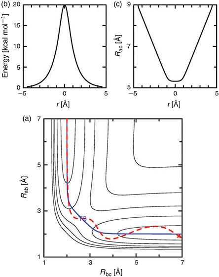
Chemists mostly consider reactions using a single nuclear coordinate, the reaction coordinate.[1] A simple example of this is apparent in the London–Eyring–Polanyi–Sato[2] (LEPS) potential-energy surface for the chlorine atom-exchange reaction[3]

that is shown in Fig. 1a as a function of the bond lengths Rab and Rbc. The reaction coordinate indicates the lowest-energy path that connects reactants to products and is shown in blue in the figure. When a reaction occurs, molecular geometries change holistically, and this coordinate in general is therefore complex, embodying what happens to all atoms including atoms in any solvent or surrounding medium. All other motions are thought to smoothly and perhaps even instantaneously adjust to motion along the reaction coordinate. Fig. 1b displays the energy profile[3] for the chlorine atom-exchange reaction as a function of the reaction coordinate, showing how the energy increases from that at the floor of the reactant valley as the approaching atom gets closer to the molecule, going through a maximum at the reaction’s transition state (TS). However, Fig. 1c shows how the distance Rac between the non-interacting atoms change along this path adjusts too. Also, this surface is shown as a two-dimensional representation for a collinear reaction but a bending coordinate would in general also be involved in the process.
|
So chemical reactions involve nuclear motions of two fundamentally different types: those that specify the reaction, and those that accompany it. Accompanying coordinates can seldom be completely ignored. Fig. 1a shows why this is so, plotting the course of a chlorine atom-exchange reaction. Initially, the system is in the reactant valley and given enough motion along the direction of the reaction coordinate to react. Indeed, a reaction ensues but the product Cla–Clb molecule is set vibrating - it is not possible to have motion purely along the reaction coordinate. Hence the properties of the other motions must affect the details of the reaction.
The nature of the reaction coordinate can change during the reaction, for example in Fig. 1 it is initially dominated by Rab, becomes the antisymmetric normal mode Rab - Rbc, and then finally becomes just Rbc. More generally, even the type of motion can change, for example if solvent must organise to make precursor complexes that facilitate breaking and making the main bonds. In addition, the electrons are also thought to follow the nuclei smoothly and regularly according to the Born–Oppenheimer principle.[4] This is not always the case, however, as, for example, a proton transfer reaction can proceed in this way but more often the proton and the electron move independently in a two-step coupled process.[5,6] In general, just as Fig. 1 shows coupling between two different nuclear motions, so nuclear and electronic motions can be coupled in a process known as vibronic coupling.[7–12]
The most obvious situation in which vibronic coupling is critical is the case of electron-transfer reactions, as captured in the adiabatic electron-transfer theory of Hush.[13–17] For such reactions, the electronic label defines the reaction, e.g.,

but the various neutral and ionic species involved have different nuclear geometries and solvation environments[18] and it is the interchange of these that constitute the reaction coordinate.[13–17]
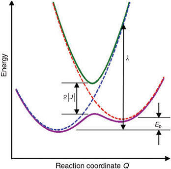
The classic depiction of an electron-transfer process is shown in Fig. 2 where the energy of the reactants, products, and intervening transition state are shown as a function of the reaction coordinate. Whilst in Fig. 1 the reactants and products are species separated an infinite distance, here the reactants and products are bound species represented by harmonic potential-energy surfaces (dashed lines, called diabatic surfaces) that are coupled together to make Born–Oppenheimer ground-state and excited-state surfaces (solid lines, call adiabatic surfaces). Coupling between the diabatic surfaces is required by quantum mechanics as the Uncertainty Principle tells us that it is not possible to confine an electron purely to just one of the two parts A or B. This coupling is given the symbol J and acts to delocalize the electron. However, such delocalization costs energy to produce, and this is measured by the reorganization energy λ shown in Fig. 2. Chemistry is a fine balance between these forces – the quantum mechanical drive to delocalize charge, and the energy needed to distort bonds so as to facilitate the delocalization.
|
Adiabatic and diabatic potential-energy surfaces have been used to describe chemical processes since immediately after the emergence of the quantum theory of matter.[1,4,19–26] The adiabatic approach is taken in quantum-chemistry packages as this allows the properties of the electrons to be determined at any nuclear configuration. It does not include the effects of nuclear momentum on the electronic structure, however, neglecting the possibility that a ‘collision’ of an electron with a nucleus can deflect the course of the nuclear motion. In the adiabatic approximation, the electronic structure adjusts instantaneously as the nuclei move. Diabatic potential-energy surfaces assume that the properties of the electrons are independent of some critical nuclear motion. The electronic structure therefore does not change as this motion occurs, meaning that the nuclear momentum cannot affect it. In the electron-transfer problem considered above, the diabatic surfaces see the electronic structures of the A and B as being either pure radical states A• and B• that are covalently bonded or else as pure singly charged states like A+ and B– that are purely ionically bonded. For example, as the NaCl molecule in the gas phases is stretched from its equilibrium geometry, the adiabatic electronic structure changes continually from a large-dipole, ionic form to a low-dipole radical form.[27,28] The ionic/radical diabatic states do not change during this process, but the adiabatic states are made by mixing the diabatic states together in different amounts, and it is this mixing that gives rise to the observed complex adiabatic-state properties. Diabatic states are used to provide chemical intuition and the language of undergraduate textbooks, defining quantities such as resonance energies (also known as electronic couplings and reorganization energies), whereas adiabatic states better reflect complex reality. However, diabatic states do not suffer from the problem of neglect of the effects of nuclear momentum that limit adiabatic states, and when the electronic coupling between the diabatic states is very weak, these states can actually better reflect experimental reality. There have been many reviews of the properties of adiabatic and diabatic states.[27,29,30]
For diabatic models, Hush showed that the ratio 2J/λ is critical to qualitative understanding.[31] For symmetric systems (energy change on reaction ΔE = 0) then, if 2|J|/λ > 1, the electronic coupling dominates and the adiabatic surfaces have a single minimum. The first molecule whose properties were interpreted in this was the Creutz–Taube ion (Chart 1)[32] in which the valence states of the Ru atoms appear to be II1/2, although details are still under discussion.[33,34] For asymmetric reactions a similar situation applies, though the details are more complicated.[35] Alternatively, when 2|J/|λ < 1 the adiabatic surfaces depict a standard double-well potential with a transition state, as shown for example in Fig. 2. The rate constant k of the chemical reaction is then given by transition state theory as
where kβ is Boltzmann’s constant, h is Planck’s constant, T the temperature, and  is the free energy of activation. As entropy variations during electron-transfer processes are typically small, this free energy can be expressed as[15,36]
equations that are exact if either E0 = 0 (symmetric reactions) or J = 0 (weak coupling) and otherwise accurate anywhere away from the region in which the transition state disappears and a single well potential results. The disappearance of the transition state generates a pitchfork bifurcation, while the transition state region forms a cusp separating the reactants and products from each other. In the limit of 2|J/|λ  1, this cusp region becomes very narrow,[15] invalidating the Born–Oppenheimer approximation and hence transition state theory. The properties of the cusp then control the reaction rate[35]: the reaction still proceeds but increasingly slowly as the coupling diminishes,[36] with the overall rate constant being given by
When no transition state forms, Eqn 4 still applies,[37] and therefore Eqn 5 also.
|
An important feature of Fig. 2 is that it shows both ground-state and excited-state potential-energy surfaces and the relationship between them. In traditional chemical thinking, different potential-energy surfaces are taken to be independent of each other, making for example UV-vis transition energies to excited states independent of ground-state properties. However, Hush showed that these properties can be intimately connected,[38] allowing the energy, intensity, and widths of observed electronic transitions to be interpreted in terms of couplings J and reorganization energies λ. Hence ground-state electron-transfer reaction rates could be predicted based upon observed spectroscopic properties. This lead to the identification of the nature of unassigned bands in dyes such as Prussian Blue,[38] inspiring the synthesis of the Creutz–Taube ion[32] and leading eventually to the understanding of how solar energy is converted to electrical energy during natural photosynthesis and in organic photovoltaic devices.
Adiabatic electron-transfer theory offers integration of a very wide range of ground-state and excited-state properties, providing analytical expressions depicting many different effects.[35,39] The similarity of the energy profile of general chemical reactions offers the possibility that most chemical processes could be similarly described, with just a few parameters providing comprehensive analysis of different chemical and spectroscopic processes. From the beginnings of chemical understanding in terms of quantum theory, such a description has been anticipated.[20–24] Indeed, general chemical reactions are often thought of this way,[30,40–54] and there exists a smooth link[55] to the reaction force model[56–58] that finds physical insight within reaction energy profiles as a function of the reaction coordinate.
A significant feature of electron-transfer in the Creutz–Taube ion is that the reaction coordinate is not dominated by intramolecular motions or indeed even by motions of the dominant atoms, as is the chlorine atom-exchange reaction. Instead, the reaction coordinate is dominated by a collective fluctuation in the coordinates of the surrounding solvent. These effects may be modelled quantitatively for both the Creutz–Taube ion[59] and general systems relevant to solar-energy conversion and organic conductivity[60] using non-equilibrium solvation methods that derive from Marcus’ original analytical treatment.[18] Indeed, any reaction that involves changing charge distributions along the reaction coordinate will be sensitive to environment, providing for example a key mechanism allowing protein structure to catalyze reactions in enzymes.[61,62] While motions accompanying intramolecular processes in the gas phase could remain coherent for extended periods, delivering sharp high-resolution spectroscopic transitions, motions in condensed phases are naively expected to decohere quickly and hence only produce broad spectral features. Neglecting any chance of coherence, processes in condensed phases are often described using harmonic baths, known in Physics as the Holstein model,[63] leading to a wide range of useful analytical solutions explaining condensed-matter phenomena.
However, application of these general diabatic concepts to problems other than electron-transfer has historically shared only limited success. Always it was possible to model single properties of systems quantitatively, providing a simple description to an otherwise complex-looking problem. The shortcoming was that different properties of the same system could not be simultaneously understood using the same set of model parameters, and that therefore it was not possible to compare one chemical system to another. Recently[39] we solved these issues by showing that general chemical reactions differed from electron-transfer typically in one fundamental way: only one electron is involved in the reaction during most electron-transfer processes, whereas two or more paired electrons are usually involved in general reactions. It is the electron count that makes the difference, rescaling the effects that the electronic coupling, reorganization energy, etc., have on the chemical and spectroscopic properties, and a key feature is that the magnitude of the rescaling is property dependent. Once this effect is factored into the analysis, many properties of the same system can be unified, and different types of chemical processes can be compared with each other. This led to an understanding of the effects of the Born–Oppenheimer approximation (i.e. the effects of the nuclear momentum on the electronic wave functions) across the whole range of feasible chemical processes,[35] an understanding of how quantum entanglement can be used to gauge the magnitude of Born–Oppenheimer breakdown,[64] and an understanding of what types of chemical reactions are likely to be of practical use in the construction of chemical qubits in a quantum information processor.[65]
Such analytical models usually focus on just the primary nuclear motion involved in the chemical process, the reaction coordinate. For all the different reactions considered, it takes on a different form, as illustrated in Fig. 3. Electron-transfer between the two metal atoms in the Creutz–Taube ion changes all of the Ru–N distances as well as reorganizing the surrounding solvent molecules, and the antisymmetric combination of these motions make up the reaction coordinate. Another reaction that can be treated is the inversion reaction in ammonia, or indeed any related isomerization process. For NH3, the reaction coordinate is the improper torsional angle depicting the umbrella motion of the molecule. Of particular interest too is the scenario with 2|J/|λ > 1 that leads to a single-welled ground-state surface instead of a double-welled one. A very well known general example of this is the structure of benzene. If benzene existed as the two cyclohexatriene Kekulé structures in thermal equilibrium, it would behave analogously to ammonia inversion. Instead, the electronic coupling (commonly called the resonance energy) is larger than the reorganization energy (2|J|/λ = 3.3)[39] and hence benzene is aromatic. For NH3, 2|J|/λ ≈ 0.85 and so the molecule takes on the pyramidal structure,[39,66] but for NH3+ 2|J|/λ = 1.05 and so the ammonia cation is planar and has maximum symmetry, akin to benzene.[66] The properties of NH3 are very different to those of PH3-BiH3, with, for example, the HXH bond angle being 108° in NH3 and 90–93° in the others.[66] This arises because the resonance integral J is much larger in NH3, favouring delocalization, owing to valence-orbital Rydbergization.[67] This process is well known when it comes to considering the spectroscopy of NH3, which is also quite different to that of the other molecules. The lowest-energy Rydberg orbital is lower in energy than the σ*XH antibonding orbital for NH3 but higher in energy for the others. The reversed ordering causes the antibonding orbital to be compressed in NH3, forcing up the resonance energy as this involves the repulsion of electrons within electron-pairs and so is very sensitive to orbital compression. Our generalized treatment therefore describes many observed phenomena. For other chemical systems, the hydrogen-bond is symmetric in the protonated ammonia dimer N2H7+ (benzene like), with EOM-CCSD/6–311++G** calculations suggesting 2|J|/λ = 1.05, so close to unity that the molecular structure is tenuously defined. The Creutz-Taube ion is double welled as 2|J|/λ ≈ 0.8 (but unlike NH3 with a similar value of 2|J|/λ, for this molecule the potential is insufficiently deep to support zero-point vibration).[34] Also the prototype molecular conducting material Alq3 (mer-tris(8-hydroxyquinolinato)aluminum(iii)) (Chart 2) has 2|J|/λ ≈ 0.08 for its strongest-coupled nearest-neighbour charge-transfer process, whilst the bacterial photosynthetic reaction-centre special-pair radical cation (Chart 3) has 2|J|/λ ≈1.8 and so the charge is delocalized over the two molecules.[39,65]
|
|
|
The connection made originally between chemical spectroscopy and chemical reactivity[38] embodied approximate analytical relationships which can be generalized,[68] used as a basis for understanding modern Stark-spectroscopy measurements,[69,70] and applied numerically using accurate full-quantum spectral simulations[68–71] based on vibronic-coupling theory.[7,8,11,12] Earlier treatments focussed on just the spectroscopy associated with the reaction coordinate,[38,71] while later ones included the other nuclear motions accompanying the electron-transfer as well.[68,72] Considering the spectroscopy of benzene highlights an important role that the accompanying modes play: excitation of benzene to its lowest excited state causes the geometry to change as the bond strength is lowered and so bonds become longer and more floppy.[73] Projecting the atomic displacements onto the normal modes of the molecule generates the Franck–Condon factors[74] that specify the intensities of all the vibrational lines observed in the spectrum. If just the Kekulé mode ν14 depicting the reaction coordinate is considered, then the spectrum would be very sharp as 2|J|/λ > 1 whereas in fact the accompanying modes make it quite broad. This is a general result. The most interesting feature of the Kekulé mode is that its frequency increases from 1309 cm–1 in the ground state[75] to 1563 cm–1 in the first excited state,[76,77] indicative of the underlying Kekulé reaction possibility.[50–54] Using an electron -transfer analogy, the first excited state has been labelled the ‘twin state’ of the ground state.[50–54] However, recently we have shown that this general concept is very helpful but the actual ‘twin state’ is the very high energy quadruply excited HOMO to LUMO excitation, not the first excited state.[39]
Even full-scale modelling of the motion just in the direction of the reaction coordinate can be cumbersome. It is easier for dissociative reactions like the Cl atom-exchange reaction (Eqn 1) as quantum scattering effects are rarely considered, allowing classical mechanics to be used to understand reaction dynamics. If the reactants and products are bound species describable as in Fig. 2, then the quantum nature of the reactant and product vibrations will have significance. Analytical theories using just the reaction coordinate describe critical high-temperature properties without the need to go into details, but for full-scale modelling or for processes at ‘low’ temperatures, the details become important. Just like the spectrum of benzene is determined by the Franck–Condon factors that project the geometry difference between the ground and excited states onto the normal modes of vibration of the molecule, so motion along the reaction coordinate needs to be projected and then each mode treated separately.
How to extend single-mode theories of spectroscopy[8–10,71] is straightforward,[11,12] but Eqn 5 is derived[36] only in the high temperature limit and its extension requires considerable effort.[78] What is meant by the ‘high temperature limit’ is that all of the motions that contribute to the reaction coordinate have frequencies less than  = 206 cm–1 at room temperature. Most intramolecular motions are of much higher frequency than this, while most solvent motions are of lower frequency, though there are exceptions in both cases. For example, in aqueous solution the dominant modes coupled to charge-transfer in the Creutz–Taube ion are the ~800 cm–1 librational modes.[34] Very large molecules will have low frequency coupled modes, but typically high frequency modes like C–C bonds and ring modes dominate molecules the size of porphyrins, chlorophylls, acenes like pentacene, Alq3, etc., that are commonly used in charge transport systems.
The number of practically significant systems to which Eqn 5 actually applies is therefore quite limited, with quantum treatments of the motion along the reaction coordinate generally being important.[78] However, this equation is widely used and mostly gives good results. This situation arises through the fortuitous cancellation of many large errors made during the calculations,[79,80] especially in calculations for electron-transport reactions in materials.[81] Whilst weak couplings can drive many biochemical processes,[82] functional materials, critical photosynthetic machinery, and artificial photovoltaics usually rely on fast processes associated with large couplings across transition states, and for these Eqn 5 is likely to fail, predicting rates in excess of those from transition state theory (Eqn 3). The challenges facing accurate calculations of materials properties has recently been reviewed.[81]
Using treatments that embody the quantized nature of molecular vibration, the role of the reaction coordinate, and the role of accompanying motions, it is possible to interpret, predict, and revise properties of important charge-transfer systems. We consider three examples: photochemical primary and secondary charge-separation and charge-recombination reactions in photosynthetic model compounds in solution, the effects of site-directed mutagenesis on the output voltage of the photochemical reaction centre from Rhodopseudomonas sphaeroides, and charge transport through the organic conductor Alq3 used in organic light-emitting diodes and photovoltaics, etc.
Many photosynthetic model compounds have been made mimicking photosynthesis, initially leading to a clear understanding of how the observed natural processes could occur,[83] but in modern times focusing on new materials for using solar energy to either produce electricity or else to perform chemical reactions to say capture CO2 or produce H2 and other fuels.[84–87] A quest was for the synthesis of a molecule that could perform long-distance photochemical charge separation and keep the charges separated for as long as possible. This would then allow for intermolecular processes to harvest the charges before recombination occurs. A record holder in this field was the ferrocene-porphyrin-fullerene triad Fc-ZnP-C60 (Chart 4) synthesized by Crossley et al. that is capable of separating charge as Fc+-ZnP-C60– for 1 ms.[88] Initially this charge-separation was assumed to occur on the singlet manifold,[88] as is most usual. However, full quantum simulations of the rate constants made by calculating the electronic couplings, reorganization energies, and the nature of the vibrational modes that constitute the reaction coordinate and its accompanying motions indicated that the rate constant on the singlet manifold should be six orders of magnitude faster. Subsequent time-resolved spectroscopic experiments found the anticipated singlet process and measured all of the rate constants for both it and the 1 ms process.[60] Many new experiments and calculations then confirmed that the 1 ms process is of very low quantum yield and occurs on the triplet manifold, despite the very rapid spin depolarization normally associated with the ferrocene cation.[60]
|
The final observed kinetics scheme is shown in Fig. 4, indicating how the various photochemical charge-separation and charge-recombination processes operate. The critical parameters deduced from the experiments and calculations for the charge recombination Fc+-ZnP-C60– → Fc-ZnP-C60 are: λ = 0.7–1.0 eV (obs.) 0.77 eV (calc.), singlet state J = 1.7–2.0 cm–1 (obs.) 31 cm–1 (calc.), triplet state J = 0.0033–0.0040 cm–1 (obs.) 0.039 (calc.). The differences between the observed and calculated couplings are of an order of magnitude, which is unusually large, but this is still small enough to be useful; the observed data is also somewhat uncertain owing to the unknown accuracy of the approximations used to interpret the observed rate constants.[60] In total 17 vibrational modes were used in these calculations, taking the most active modes describing the change in the geometries of the ferrocene, porphyrin, and fullerene structural components accompanying charge transfer to/from these groups. Density functional theory (DFT) was used for most calculations but complete-active-space self-consistent-field calculations were used to obtain the spin-orbit allowed triplet charge-recombination couplings.
|
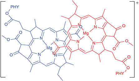
Next we consider the properties of the special-pair radical cation from Rhodobacter sphaeroides (Chart 3). The ‘special pair’ is a bacteriochlorophyll dimer to which the surrounding antenna complexes transfer their absorbed solar energy. This dimer initiates primary charge separation, ejecting an electron to nearby molecules, leaving behind a radical cation. The redox potential of this radical cation is an important contributor to the output voltage available to do chemical work subject to the light absorption. How the protein environment acts to control this redox potential is therefore a significant aspect of the photosynthetic process. An experimental handle on this was obtained using site-directed mutagenesis to make 30 mutants of the surrounding protein, changing the electrostatic environment around each of the bacteriochlorophylls and so modulate ΔE.[89,90] This changes the charges ρL and ρM on the two bacteriochlorophylls; ‘L’ and ‘M’ are the names of the protein chains to which the two macrocycles bind, and the net charge is ρL + ρM = 1. These charges were measured by spin-resonance spectroscopy. Mutation also changes the midpoint potential Em, which was monitored by electrochemistry. Six series of mutants were obtained by replacing residues at six different protein sites. The results for four of these series are shown in Fig. 5.
|
Independently, the intervalence hole-transfer band of the special-pair radical cation, akin to the band identified by Hush in Prussian Blue and made famous by the Creutz–Taube ion, was measured.[91–93] We modelled this spectrum using vibronic coupling theory.[94] The natures of the reaction coordinate and the primary accompanying modes were calculated using DFT, and 50 modes selected to describe the reaction coordinate with a further 20 included to describe the accompanying modes.[95] Major controlling parameters such as the electronic coupling J between the two bacteriochlorophylls, the associated reorganization energies λA in the reaction coordinate and λS in the accompanying modes, as well as the mutation-dependent site energy difference ΔE, were calculated a priori and then the values adjusted slightly to fit the observed spectrum.[94] Two nearby interfering electronic states were also required to be identified and then fully included in these calculations.[96]
This interpretation of the intervalence spectrum yields immediately the midpoint potential and the charge and spin distributions. Knowing the location of the mutated sites, the dipole moments of the amino acids involved in the mutation, and the dielectric constant then tells how the site asymmetry ΔE is affected by mutation, allowing the midpoint potential and spin distribution to be calculated for each mutant. The predicted correlations[97] are also shown on Fig. 5 and are in agreement with the experimental data to within the observed error bars. These results were obtained by numerical solution to the full quantum coupled nuclear-electronic motion problem and involved finding the spectrum of matrices of dimension ~107. It is also possible to obtain analytical solutions for the case in which the reaction coordinate and the accompanying motions are described by a single mode each, leading to[98]

This result is also shown in the figure using actual rather than fitted parameters,[97] utilizing basic results from adiabatic electron-transfer theory that allow the densities to be determined from the model parameters.[15] The analytical solution captures all the key qualitative features but is not quantitatively predictive. Nevertheless, it highlights how easy it is to capture the key chemical features controlling solar energy conversion using simplistic models. It also captures the importance of the accompanying modes that contribute to λS, placing them on an equal footing to the modes contributing to the reaction coordinate, λA. Another way of modulating the site asymmetry is via Stark spectroscopy. Our models predicted that these spectra would vary dramatically between different mutants, with these predictions later being quantitatively verified.[99]
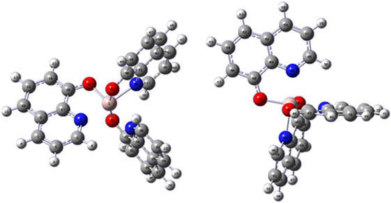
The third example considered is the conductivity of Alq3 material. Calculations focusing on doing the best job possible with each of the many terms contributing to the conductivity are capable of predicting mobilities to within an order of magnitude of observed values.[81] This is useful as different crystalline and amorphous structures can have mobilities varying over eight orders of magnitude. Each molecule has an irregular shape that can pack into crystalline arrays but commercial products are amorphous. Even in the crystal the intermolecular packing produces many different types of intermolecular arrangements, with one molecular pair shown in Fig. 6 to highlight the general lack of regularity. Consequently, conductivity is highly anisotropic. Extensive quantum calculations require the inclusion of 10–20 vibrational modes to describe the motion along the reaction coordinate and major associated coordinates. They yield rate constants for the passage of charge from one site to one of its neighbours, and then the classical master equation describing the kinetics of charge flow through the material is solved in the presence of an external driving electric field. Most intermolecular interactions are poorly suited to charge transport and so calculated rate constants can be as low as 107 s–1. However, some times the aromatic ligands stack perfectly and then the high-temperature explicit-vibration version[78] of Eqn 5 predicts rate constants up to 1014 s–1, greater than the transition state theory rate by over an order of magnitude and greater than the observed maximum rate by the same amount. When molecular conductors like Alq3 conduct well, they do it adiabatically over transition states.[81]
|
These three examples of electron-transfer processes all have well defined reaction coordinates. Indeed, most chemical reactions also have well defined paths from reactants to products. However, this is not always the case and we will finish with two further examples for which the nature of the accompanying motions is obvious whilst the actual identity of the chemical process is obscured. These come from photochemistry applications to which basic chemical intuition is not always readily applicable. The first example concern photofragmentation of the pyridinium ion in the gas phase, the second concerns what happens to the energy of a chlorophyll molecule in solution or in situ when it is excited in its Qx (S2, orange) absorption band.
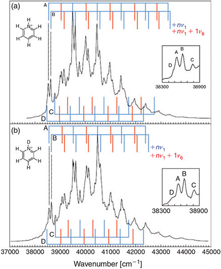
Pyridinium ions photoexcited to their lowest singlet excited state dissociate, loosing H2.[100] The key question is: how does this occur? (i.e. what is the nature of the reaction coordinate?)Photodissociation of simple molecules like I2 is taught in most undergraduate courses. For this the reaction coordinate is obvious – the I–I stretch – and the observed spectra reveal all there is to know about the reaction. One would naively think that this would also be the case for pyridinium, but rarely is it that simple as the observed spectra pertaining to polyatomic-molecule photochemistry tend to be dominated by the accompanying motions rather than the reaction coordinate itself. Fig. 7 reproduces observed spectra for two molecular isotopes.[100] These spectra can be readily assigned as depicting Franck–Condon progressions in the symmetric modes ν1 and ν6 (see Fig. 7). However, the reaction coordinate generally describes antisymmetric motions (like Rab - Rbc at the transition state in Fig. 1) and so symmetric modes by their very nature are usually only accompanying modes.
|
The observed progressions are based on four apparent origins named A–D in the figure. It is possible that one of these is the true 0–0 origin of the spectrum and that the other three lines, naively unexpected in the spectra, provide information as to the nature of the reaction coordinate. High-level ab initio and density functional calculations are inconsistent with this interpretation, however. Instead, they reveal that the excited-state potential-energy surface contains a deep double well. Significantly, the transition moment to levels at the bottom of the double well is calculated to be very small. The first levels with sufficient intensity to be seen are at energies near the transition state, with four levels predicted akin to what is observed. No simple relationship explaining the frequency differences exists, however, and plausible lines that would reveal the nature of the motion along the reaction-coordinate double-well are too weak to be observed. Nevertheless, these dark states contribute significantly to the observed photochemistry.[100]
The final example concerns the visible region of the absorption spectrum of chlorophyll-a and indeed all of the chlorophyllide series of molecules.[101] This is the primary absorption driving natural photosynthesis. All investigations of exciton transport, primary charge separation, and quantum coherence in natural photosynthesis pertain to it. Two independent electronic transitions contribute to the absorption; these are sometimes well separated, as in e.g. bacteriochlorophyll-a and pheophytin-a, but sometimes overlapping, as in the most important chlorophyllide, chlorophyll-a. They are named Qy (the lower-energy band) and Qx, and the main question concerns just where these two absorptions lie, their relative intensities, and what happens to the light after it is absorbed by the higher-energy band Qx. The answers to these questions will profoundly influence exciton transport and quantum coherence properties. Absorption to Qx must lead to a photochemical reaction, and the nature of the reaction coordinate is of primary interest.
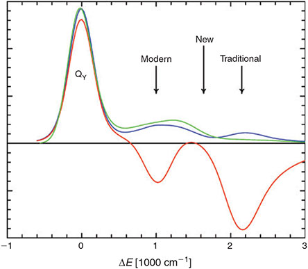
Some critical experimental data taken for chlorophyll-a in ether at room temperature is shown in Fig. 8.[102,103] The Q-band absorption contains three broad peaks, a dominant peak associated with the Qy origin, and two weaker ones located higher in energy by +1400 and +2150 cm–1. Both of these contain Qy sideband character, as evidenced by the shown reflected Qy emission spectrum. If the normal vibrational modes of the ground and excited-states are the same, then the absorption and reflected emission spectra would precisely overlap, but Duschinsky rotation of the modes occurs and this can have a profound effect on sideband shape and intensity, as evidenced in detail for bacteriochlorophyll-a.[104] The significant enhancement of the absorption intensity at +2150 cm–1, combined with other evidence, led to the 1960s assignment of the Qx origin at this location. This has been called the ‘traditional’ assignment. If Qx is located this far from Qy then Qy will dominate all exciton transport and coherence properties of photosystems, and this assignment has been used in all such analyses to this present day.
|
Also shown in Fig. 8 is the magnetic-circular-dichroism (MCD) spectrum of chlorophyll-a in ether.[102] This is like the absorption spectrum except that Qx subtracts from Qy instead of adding to it, and the relative intensities are different with the two bands being of roughly equal importance in the MCD but Qx being relatively weak in absorption. The large negative signal at +2150 cm–1 expected from the traditional assignment is obvious, but a second unexpected negative signal also appears at +1000 cm–1. The origin of this signal was never clear and the traditional assignment could not account for it. In the 1980s, the traditional assignment was replaced by the ‘modern’ one in which Qx is assigned to the +1000 cm–1 peak instead. Much experimental data supported this assignment, but it struggled to explain the observation of a second negative MCD band, just as did the traditional assignment. If Qx is located at +1000 cm–1 then the implications for exciton transport and coherence in photosystems would be significant and its inclusion in analyses of experimental data would be essential.
The basic issue was that the ‘traditional’ and ‘modern’ assignments did not consider the underpinning photochemical reaction that occurs when Qx is excited, focusing only on the accompanying motions, motions clearly identifiable in the spectra. We showed that it was the vibronic coupling in the reaction coordinate that is responsible for the qualitative observation of two negative peaks in the MCD spectrum.[101] Both peaks are therefore associated with Qx and this band takes on a very unusual shape, having minimal absorption at the band centre. Our new assignment of the band centre is also shown in Fig. 8 and is highly counter-intuitive. It can explain a very wide range of experimental data measured not just for chlorophyll-a but for every other chlorophyllide too, and is fully consistent with predictions from high-level DFT and ab initio calculations. Different experiments may appear to prefer either the ‘traditional’ or ‘modern’ assignments over the other, but in reality both peaks derive equally from Qx.
Interestingly, Gouterman originally developed the theory of the effects of vibronic coupling on molecular spectra as a way of assigning the Q-band systems of the chlorophyllides,[8–10] an approach that later had a profound impact on the understanding of electron-transfer processes.[71] That the two observed bands in chlorophyll-a could be indicative of an underlying reaction coordinate was clear to him, yet the lack of observation of two negative MCD bands in most other chlorophyllides suggested that this was not the correct interpretation of the data. Indeed, the missing bands remained unobserved for 50 years until we pioneered techniques employing quantitative vibronic coupling analyses,[101] paralleled by the development of the first-ever technique permitting analytical inversion of observed MCD and absorption spectral data to yield the critically required state polarization information.[105] Both of these methods allow for quantitative identification of all expected bands, verifying the vibronic coupling hypothesis. Another significant obstacle that was overcome concerned the interpretation of many highly influential spectra, measured over 30 years, of chlorophyll-a in ether at low temperature. These had led to the original proposal of the ‘modern’ assignment and the same arguments also favoured it over our ‘new’ assignment. We showed that all discrepancies with our new assignment stemmed from the presence of trace water contamination in the solvent used in the experiments.[106] High-level computations conform this interpretation.[107]
The consequences of this new assignment can be minor, say when the properties of chlorophyllides like bacteriochlorophyll-a or pheophytin-a with large obvious Qx-Qy separations are considered, significant for chlorophyll-a itself, and very large for uncommon but nevertheless important photosystems utilizing bacteriochlorophyll-c, bacteriochlorophyll-d, chlorophyll-c, and others. For the first time for chlorophyll-a and most of the chlorophyllides, we were able to determine the relative absorption strengths of Qx compared with Qy. Surprisingly, this ranged over a factor of seven, greatly varying the significance of Qx to the photosynthetic activity.
Once the reaction coordinate was identified, standard kinetics theories[108] gave the rate of decoherence of Qx-absorbed radiation. This provided the first explanation of the observation that amongst all chlorophyllides, chlorophyll-a in situ in reaction centres is perfectly optimized to decohere excitation.[101] It is unclear as to whether this is an optimized evolutionary outcome or just a coincidence, but if it is an optimized outcome than the result has significant consequences for the design of artificial solar-energy utilization devices.
In conclusion, we see that adiabatic electron-transfer can now be generalized and used as a solid basis for understanding many completely different types of chemical processes including isomerization, hydrogen bonding, aromaticity, photochemistry, electron-transfer, organic conductors, and by implication most processes that occur via a transition state or via surface hopping. With smooth links to the traditional models used since the 1930s to understand chemical processes, this approach focuses on the reaction coordinate, its changing nature during the reaction, the transition state and the accompanying independent motions.
Our focus here is on the differences between the reaction coordinate and the accompanying motions, the effects that each have on spectral and kinetics properties, and the difficulties that can arise in discriminating one from the other. Focus on the accompanying modes is a recent phenomenon, dating back only 20 years.[68,72] However, their effects are nearly always critical to quantitative analysis, as revealed directly by, e.g. Eqn 6. Before this period, accompanying modes were treated empirically assuming say a Gaussian or Poisson linewidth applied to spectral transitions associated with the reaction coordinate, and indeed this may often be all that is required for qualitative and even quantitative analysis. Now, we recognise that the accompanying motions may manifest themselves in many and varied ways. At the simple end, this could mean just that they need to be included in accurate simulations but can be ignored in descriptive analytical theories that capture the essential features. However, it can also mean that the identity of the reaction coordinate itself is obscured in spectral measurements, and that proper understanding of the effects of the accompanying modes is essential to determining the most simple qualitative explanation of the observed phenomena. This is certainly the case when it comes to understanding the spectra of chlorophylls, and the inability to distinguish reaction coordinate from accompanying modes held up the development of a fundamental understanding of the operation of photosynthesis for over 50 years.
While the tight connection between chemical reactivity and chemical spectroscopy has been known now for 50 years, it is only recently that this has led to a cross-polarization of methods. Methods from molecular spectroscopy are now routinely used to solve electron-transfer problems, and just this year it has been shown how to apply the full power of electron-transfer theory to the understanding of basic concepts such as hybridization and aromaticity. Chemistry has always been taught to undergraduate students as a set of independent principles, applied as required to organic reactions, inorganic complexes, materials properties, or gas-phase reactions. This teaching introduces different languages and notations for each situation. A simpler and more unified approach seems to be on the horizon. Understanding the importance of what defines the reaction coordinate and what other motions are necessarily associated with this will be core to such a simplified description.
References
[1] H. Eyring, M. Polanyi, Z. Phys. Chem. Abt. B 1931, 12, 279.| 1:CAS:528:DyaA3MXjtF2msw%3D%3D&md5=49b7f2adc4b8fae0163af95b9877a9e5CAS |
[2] S. Sato, J. Chem. Phys. 1955, 23, 2465.
| Crossref | GoogleScholarGoogle Scholar | 1:CAS:528:DyaG28XhvVGhtg%3D%3D&md5=5259ad92ed3e5747c3b48a348a47e108CAS |
[3] J. P. Bergsma, J. R. Reimers, K. R. Wilson, J. T. Hynes, J. Chem. Phys. 1986, 85, 5625.
| Crossref | GoogleScholarGoogle Scholar | 1:CAS:528:DyaL2sXpslGq&md5=b39e22debc9a40d72600094cdd752fe5CAS |
[4] M. Born, R. Oppenheimer, Ann. Phys. 1927, 389, 457.
| Crossref | GoogleScholarGoogle Scholar |
[5] S. Hammes-Schiffer, A. A. Stuchebrukhov, Chem. Rev. 2010, 110, 6939.
| Crossref | GoogleScholarGoogle Scholar | 1:CAS:528:DC%2BC3cXhtlyhtbzN&md5=52e454ca663dba4003cf3a4b70e32966CAS | 21049940PubMed |
[6] S. Hammes-Schiffer, Chem. Rev. 2010, 110, 6937.
| Crossref | GoogleScholarGoogle Scholar | 1:CAS:528:DC%2BC3cXhsFShtbrN&md5=b6553e329e21c8a68358bd39c7886b82CAS | 21141827PubMed |
[7] G. Herzberg, E. Teller, Z. Phys. Chem. 1933, 21, 410.
[8] R. L. Fulton, M. Gouterman, J. Chem. Phys. 1961, 35, 1059.
| Crossref | GoogleScholarGoogle Scholar | 1:CAS:528:DyaF38Xkt1enug%3D%3D&md5=afaa9792498299c6b982eb2f43f799faCAS |
[9] R. L. Fulton, M. Gouterman, J. Chem. Phys. 1964, 41, 2280.
| Crossref | GoogleScholarGoogle Scholar | 1:CAS:528:DyaF2cXkslektLs%3D&md5=e41f05166b973ac34b007f98583fdf78CAS |
[10] M. Gouterman, J. Chem. Phys. 1965, 42, 351.
| Crossref | GoogleScholarGoogle Scholar | 1:CAS:528:DyaF2MXhvFKrug%3D%3D&md5=54355b71d0657130f5f2a184cec76ed0CAS |
[11] I. G. Ross, Isr. J. Chem. 1975, 14, 118.
| Crossref | GoogleScholarGoogle Scholar | 1:CAS:528:DyaE28Xhsl2gu7o%3D&md5=3658d37763829bf1176f81d9ee649e9dCAS |
[12] G. Fischer, Vibronic Coupling 1984 (Academic Press: London).
[13] N. S. Hush, in Soviet Electrochemistry: Proceedings of the Fourth Conference on Electrochemistry 1956 (Ed. A. N. Frumkin) (English translation: Consultants Bureau, New York) 1961, Vol. 1, pp. 99–100 (Trudy 4-go soveshchaniia po elektrokhimii 1-6 oktiabria 1956, published by Izd-vo Akademii nauk SSSR, Moskva, 1959).
[14] N. S. Hush, Z. Elektrochem. Angew. Phys. Chem. 1957, 61, 734.
| 1:CAS:528:DyaG2sXovFCqtw%3D%3D&md5=29c65f82c338688d58be6a0500926a0eCAS |
[15] N. S. Hush, J. Chem. Phys. 1958, 28, 962.
| Crossref | GoogleScholarGoogle Scholar | 1:CAS:528:DyaG1cXptFKitA%3D%3D&md5=2190839bbaac51e0fb5294313a628a2fCAS |
[16] N. S. Hush, Trans. Faraday Soc. 1961, 57, 557.
| Crossref | GoogleScholarGoogle Scholar | 1:CAS:528:DyaF3MXhtV2ksrg%3D&md5=dc0e438210b372799863761530485edeCAS |
[17] N. S. Hush, J. Electroanal. Chem. 1999, 460, 5.
| Crossref | GoogleScholarGoogle Scholar | 1:CAS:528:DyaK1MXhs1Sls7c%3D&md5=1d8659fd618daa5e05af1db81f376e35CAS |
[18] R. A. Marcus, J. Chem. Phys. 1956, 24, 966.
| Crossref | GoogleScholarGoogle Scholar | 1:CAS:528:DyaG28XmtlWksw%3D%3D&md5=888b1d4eae363fda5b9e568e22eb2140CAS |
[19] F. London, Z. Phys. 1928, 46, 455.
| 1:CAS:528:DyaB1cXhtlSmsA%3D%3D&md5=45540de3eab83c1a3f7832d02de6a88cCAS |
[20] M. G. Evans, M. Polanyi, Trans. Faraday Soc. 1938, 34, 11.
| Crossref | GoogleScholarGoogle Scholar | 1:CAS:528:DyaA1cXitVWisg%3D%3D&md5=4ca755b360055e3fe246fedcf7cb70e5CAS |
[21] J. Horiuti, M. Polanyi, J. Mol. Catal. A: Chem. 2003, 199, 185.[translation of Acta Physicochimica U.R.S.S. 1935, 2, 505]
| Crossref | GoogleScholarGoogle Scholar | 1:CAS:528:DC%2BD3sXjsVGmu7w%3D&md5=1709003d2681250a5a78c685fdde6e7bCAS |
[22] F. T. Wall, G. Glockler, J. Chem. Phys. 1937, 5, 314.
| Crossref | GoogleScholarGoogle Scholar | 1:CAS:528:DyaA2sXjt1KntA%3D%3D&md5=2dcbce9553a258fbc87f56e346744b0cCAS |
[23] N. S. Hush, J. Polym. Sci., Polym. Phys. Ed. 1953, 11, 289.
| 1:CAS:528:DyaG2cXitVyltA%3D%3D&md5=dc3dad120e212e4f2ade1ae644dd36abCAS |
[24] F. London, Z. Phys. 1932, 74, 143.
| Crossref | GoogleScholarGoogle Scholar | 1:CAS:528:DyaA38XjtVWqtg%3D%3D&md5=9918be9fd3b02b13fa95feb049cdd5c7CAS |
[25] L. D. Landau, Phys. Z. Sowjetunion 1932, 2, 46.
| 1:CAS:528:DyaA3sXhvFGk&md5=22d4dfa4a81f0e83dbb9832c2f5aad24CAS |
[26] L. D. Landau, Phys. Z. Sowjetunion 1932, 1, 88.
| 1:CAS:528:DyaA38XktlOntQ%3D%3D&md5=4b13540001c400f83df96f081e72e020CAS |
[27] T. Van Voorhis, T. Kowalczyk, B. Kaduk, L.-P. Wang, C.-L. Cheng, Q. Wu, Annu. Rev. Phys. Chem. 2010, 61, 149.
| Crossref | GoogleScholarGoogle Scholar | 1:CAS:528:DC%2BC3cXmt1WrsbY%3D&md5=a98c415c01fabd714d67441e69a6d06eCAS | 20055670PubMed |
[28] E. J. Barton, C. Chiu, S. Golpayegani, S. N. Yurchenko, J. Tennyson, D. J. Frohman, P. F. Bernath, Mon. Not. R. Astron. Soc. 2014, 442, 1821.
| Crossref | GoogleScholarGoogle Scholar | 1:CAS:528:DC%2BC2cXhtFShsL3J&md5=67e2b246183d7ee495f61640ffe2d04dCAS |
[29] S. B. Piepho, P. N. Schatz, Group Theory and Spectroscopy 1983 (Wiley: New York, NY).
[30] I. B. Bersuker, Chem. Rev. 2013, 113, 1351.
| Crossref | GoogleScholarGoogle Scholar | 1:CAS:528:DC%2BC3sXms1yisg%3D%3D&md5=2b96e9728b5bf9daa602e89dd63c7469CAS | 23301718PubMed |
[31] N. S. Hush, NATO Adv. Study Inst. Ser., Ser. C 1980, 58, 151.
| 1:CAS:528:DyaL3MXlslaiuw%3D%3D&md5=ba76ae94aa0fad0eb9223cccf51ac0dbCAS |
[32] C. Creutz, H. Taube, J. Am. Chem. Soc. 1969, 91, 3988.
| Crossref | GoogleScholarGoogle Scholar | 1:CAS:528:DyaF1MXltVGgs7o%3D&md5=3a328762ba88ef246939730040d82b49CAS |
[33] K. D. Demadis, C. M. Hartshorn, T. J. Meyer, Chem. Rev. 2001, 101, 2655.
| Crossref | GoogleScholarGoogle Scholar | 1:CAS:528:DC%2BD3MXms1ersrY%3D&md5=02c6c277a0346f8f060db388ce8441a6CAS | 11749392PubMed |
[34] J. R. Reimers, B. B. Wallace, N. S. Hush, Philos. Trans. R. Soc. A 2008, 366, 15.
| Crossref | GoogleScholarGoogle Scholar | 1:CAS:528:DC%2BD1cXhsVCgsr0%3D&md5=0f8d13860541835c25601db88ee56781CAS |
[35] J. R. Reimers, L. McKemmish, R. H. McKenzie, N. S. Hush, Phys. Chem. Chem. Phys. 2015,
| Crossref | GoogleScholarGoogle Scholar |
[36] V. G. Levich, R. R. Dogonadze, Dokl. Akad. Nauk. SSSR Ser. Fiz. Khim. 1959, 124, 123.
| 1:CAS:528:DyaF3MXmtFA%3D&md5=e29f88eb0e23d1bd66f2629f3c11a657CAS |
[37] R. Kubo, Y. Toyozawa, Prog. Theor. Phys. 1955, 13, 160.
| Crossref | GoogleScholarGoogle Scholar |
[38] N. S. Hush, Prog. Inorg. Chem. 1967, 8, 391.
| Crossref | GoogleScholarGoogle Scholar | 1:CAS:528:DyaF1cXhtVSjsbY%3D&md5=0d9a6f375971a0352ce765110d4e2fc4CAS |
[39] J. R. Reimers, L. McKemmish, R. H. McKenzie, N. S. Hush, Phys. Chem. Chem. Phys. 2015,
| Crossref | GoogleScholarGoogle Scholar |
[40] I. B. Bersuker, Chem. Rev. 2001, 101, 1067.
| Crossref | GoogleScholarGoogle Scholar | 1:CAS:528:DC%2BD3MXhslagsLY%3D&md5=cc63413fb75d390f5b268bafeb8be2c1CAS | 11709858PubMed |
[41] I. B. Bersuker, Adv. Quantum Chem. 2003, 44, 1.
| Crossref | GoogleScholarGoogle Scholar | 1:CAS:528:DC%2BD2cXhsVSmu70%3D&md5=db496bc7ea6bf5e86b4fd3640de4c69dCAS |
[42] Y. Liu, I. B. Bersuker, W. Zou, J. E. Boggs, J. Chem. Theory Comput. 2009, 5, 2679.
| Crossref | GoogleScholarGoogle Scholar | 1:CAS:528:DC%2BD1MXhtFOks7fM&md5=0cc9d68bcca2bc4837a840e74b7fd255CAS |
[43] P. García-Fernández, J. A. Aramburu, M. Moreno, M. Zlatar, M. Gruden-Pavlović, J. Chem. Theory Comput. 2014, 10, 1824.
| Crossref | GoogleScholarGoogle Scholar |
[44] R. G. Pearson, J. Mol. Struct.: THEOCHEM 1983, 103, 25.
| Crossref | GoogleScholarGoogle Scholar |
[45] R. F. W. Bader, Can. J. Chem. 1962, 40, 1164.
| Crossref | GoogleScholarGoogle Scholar | 1:CAS:528:DyaF38XksVSntro%3D&md5=4ce5073c50b7d4248ac7e9fcd62cb33dCAS |
[46] L. Salem, J. S. Wright, J. Am. Chem. Soc. 1969, 91, 5947.
| Crossref | GoogleScholarGoogle Scholar | 1:CAS:528:DyaF1MXlt12htro%3D&md5=6b066dd673796442e13ea15d63aa8a11CAS |
[47] R. G. Pearson, J. Am. Chem. Soc. 1969, 91, 4947.
| Crossref | GoogleScholarGoogle Scholar | 1:CAS:528:DyaF1MXkslCitb8%3D&md5=bc59e076c18025c85202e1f8c1473189CAS |
[48] R. G. Pearson, Acc. Chem. Res. 1971, 4, 152.
| Crossref | GoogleScholarGoogle Scholar | 1:CAS:528:DyaE3MXhtlSmt74%3D&md5=ad78db7847d42145266de77b7f66ac7eCAS |
[49] C. C. Levin, J. Am. Chem. Soc. 1975, 97, 5649.
| Crossref | GoogleScholarGoogle Scholar | 1:CAS:528:DyaE2MXlvVeqsLw%3D&md5=7d1f8203dd363e234f6f18bcedf31c67CAS |
[50] S. Zilberg, Y. Haas, D. Danovich, S. Shaik, Angew. Chem. Int. Ed. 1998, 37, 1394.
| Crossref | GoogleScholarGoogle Scholar | 1:CAS:528:DyaK1cXjvFGjt74%3D&md5=8835f1a91c2b40b8c54786d5c343f45fCAS |
[51] S. Shaik, S. Zilberg, Y. Haas, Acc. Chem. Res. 1996, 29, 211.
| Crossref | GoogleScholarGoogle Scholar | 1:CAS:528:DyaK28XisVymurc%3D&md5=2775cb99ac3b5c270f54b642ad2a4607CAS |
[52] S. Shaik, A. Shurki, D. Danovich, P. C. Hiberty, J. Am. Chem. Soc. 1996, 118, 666.
| Crossref | GoogleScholarGoogle Scholar | 1:CAS:528:DyaK28XitFSmuw%3D%3D&md5=19a5270307951a6f3a3a42f7a9712277CAS |
[53] S. Shaik, A. Shurki, D. Danovich, P. C. Hiberty, Chem. Rev. 2001, 101, 1501.
| Crossref | GoogleScholarGoogle Scholar | 1:CAS:528:DC%2BD3MXis1Sqtrc%3D&md5=a33b96318007127148b72f7d3a28dff3CAS | 11710231PubMed |
[54] S. Zilberg, Y. Haas, J. Phys. Chem. A 2011, 115, 10650.
| Crossref | GoogleScholarGoogle Scholar | 1:CAS:528:DC%2BC3MXhtFSmt7vO&md5=7058d14b8e8a164810c77894d7a7cab2CAS | 21851061PubMed |
[55] P. Politzer, J. R. Reimers, J. S. Murray, A. Toro-Labbe, J. Phys. Chem. Lett. 2010, 1, 2858.
| Crossref | GoogleScholarGoogle Scholar | 1:CAS:528:DC%2BC3cXhtFGhsbvM&md5=71175bc5682923ad923806f1f912438aCAS |
[56] A. Toro-Labbe, J. Phys. Chem. A 1999, 103, 4398.
| Crossref | GoogleScholarGoogle Scholar | 1:CAS:528:DyaK1MXjtVSms78%3D&md5=9e0738862bfdfdff67e752676e130387CAS |
[57] A. Toro-Labbe, S. Gutierrez-Oliva, J. S. Murray, P. Politzer, Mol. Phys. 2007, 105, 2619.
| Crossref | GoogleScholarGoogle Scholar | 1:CAS:528:DC%2BD2sXhsVGjsb%2FN&md5=03d19b50d1249cd08f77a7abb4cf25a6CAS |
[58] A. Toro-Labbe, S. Gutierrez-Oliva, J. S. Murray, P. Politzer, J. Mol. Model. 2009, 15, 707.
| Crossref | GoogleScholarGoogle Scholar | 1:CAS:528:DC%2BC3cXlslGis7w%3D&md5=34e49fb5e3559f1b4b573e7356fda825CAS | 19085021PubMed |
[59] J. R. Reimers, Z.-L. Cai, H. S. Hush, Chem. Phys. 2005, 319, 39.
| Crossref | GoogleScholarGoogle Scholar | 1:CAS:528:DC%2BD2MXht1Ort73L&md5=2029e7edbc2e68104d79e93dca94b853CAS |
[60] S.-H. Lee, A. G. Larsen, K. Ohkubo, Z.-L. Cai, J. R. Reimers, S. Fukuzumi, M. J. Crossley, Chem. Sci. 2012, 3, 257.
| Crossref | GoogleScholarGoogle Scholar | 1:CAS:528:DC%2BC3MXhsFeju7bE&md5=c6222858034fc92fbe0f043c5bbcdb92CAS |
[61] A. Warshel, Proc. Natl. Acad. Sci. USA 1978, 75, 5250.
| Crossref | GoogleScholarGoogle Scholar | 1:CAS:528:DyaE1MXltVGnsw%3D%3D&md5=6229ec8fd16b9a18b70902a9e5c9bd88CAS | 281676PubMed |
[62] S. D. Fried, S. Bagchi, S. G. Boxer, Science 2014, 346, 1510.
| Crossref | GoogleScholarGoogle Scholar | 1:CAS:528:DC%2BC2cXitV2gtrzN&md5=b004a090802f833b80055be14e14bc2eCAS | 25525245PubMed |
[63] H. Rongsheng, L. Zijing, W. Kelin, Phys. Rev. B 2002, 65, 174303.
| Crossref | GoogleScholarGoogle Scholar |
[64] L. McKemmish, R. H. McKenzie, N. S. Hush, J. R. Reimers, Phys. Chem. Chem. Phys. 2015,
| Crossref | GoogleScholarGoogle Scholar |
[65] L. K. McKemmish, R. H. McKenzie, N. S. Hush, J. R. Reimers, J. Chem. Phys. 2011, 135, 244110.
| Crossref | GoogleScholarGoogle Scholar | 22225147PubMed |
[66] J. R. Reimers, L. McKemmish, R. H. McKenzie, N. S. Hush, Phys. Chem. Chem. Phys. 2015,
| Crossref | GoogleScholarGoogle Scholar |
[67] R. S. Mulliken, Acc. Chem. Res. 1976, 9, 7.
| Crossref | GoogleScholarGoogle Scholar | 1:CAS:528:DyaE28Xms12qsw%3D%3D&md5=3a6e688b62ecf316493ec5c97f35bddfCAS |
[68] J. R. Reimers, N. S. Hush, Chem. Phys. 2004, 299, 79.
| Crossref | GoogleScholarGoogle Scholar | 1:CAS:528:DC%2BD2cXhslWhtbk%3D&md5=5a9f09a6e0c78476f6dd6f3a4c1045d7CAS |
[69] J. R. Reimers, N. S. Hush, in Mixed Valence Systems: Applications in Chemistry, Physics, and Biology (Ed. K. Prassides) 1991, pp. 29–50 (Kluwer Academic Publishers: Dordrecht).
[70] J. R. Reimers, N. S. Hush, J. Phys. Chem. 1991, 95, 9773.
| Crossref | GoogleScholarGoogle Scholar | 1:CAS:528:DyaK3MXms1Gktr4%3D&md5=f19e6d5caa9d517c4125a901169237aeCAS |
[71] S. B. Piepho, E. R. Krausz, P. N. Schatz, J. Am. Chem. Soc. 1978, 100, 2996.
| Crossref | GoogleScholarGoogle Scholar | 1:CAS:528:DyaE1cXktFCgt74%3D&md5=2760adb9e5e368380fa5a6d457084f6dCAS |
[72] J. R. Reimers, N. S. Hush, Chem. Phys. 1996, 208, 177.
| Crossref | GoogleScholarGoogle Scholar | 1:CAS:528:DyaK28Xkt12rsbg%3D&md5=5c118f1840544ef0edeffa31a2a42af9CAS |
[73] K. K. Innes, I. G. Ross, W. R. Moomaw, J. Mol. Spectrosc. 1988, 132, 492.
| Crossref | GoogleScholarGoogle Scholar | 1:CAS:528:DyaL1MXht1eqsLY%3D&md5=5c61b33964e5d3a55855c63ed7fc3ae6CAS |
[74] E. U. Condon, Phys. Rev. 1928, 32, 858.
| Crossref | GoogleScholarGoogle Scholar | 1:CAS:528:DyaB1MXit1CisQ%3D%3D&md5=9f0b7beb680febd11e4816ab3c0ef38bCAS |
[75] A. G. Ozkabak, L. Goodman, K. B. Wiberg, J. Chem. Phys. 1990, 92, 4115.
| Crossref | GoogleScholarGoogle Scholar | 1:CAS:528:DyaK3cXit1Gltr8%3D&md5=b20d7561da9d2319ebd8a6b8e19263efCAS |
[76] D. M. Friedrich, W. M. McClain, Chem. Phys. Lett. 1975, 32, 541.
| Crossref | GoogleScholarGoogle Scholar | 1:CAS:528:DyaE28Xhs1enug%3D%3D&md5=f9f9eb044c46125d417a5acb50892d63CAS |
[77] J. Murakami, K. Kaya, M. Ito, J. Chem. Phys. 1980, 72, 3263.
| Crossref | GoogleScholarGoogle Scholar | 1:CAS:528:DyaL3cXksFOitLY%3D&md5=a8b05d4a077ff314162036266fc42404CAS |
[78] A. Warshel, J. Phys. Chem. 1982, 86, 2218.
| Crossref | GoogleScholarGoogle Scholar | 1:CAS:528:DyaL38Xit1Cjsrc%3D&md5=c1aa945514b0db3813fe191e38afc2cbCAS |
[79] J. E. Norton, J. L. Brédas, J. Am. Chem. Soc. 2008, 130, 12377.
| Crossref | GoogleScholarGoogle Scholar | 1:CAS:528:DC%2BD1cXhtValu7%2FN&md5=5800cf406cec1c0054e2d8dfc69bebefCAS | 18715006PubMed |
[80] G. Nan, X. Yang, L. Wang, Z. Shuai, Y. Zhao, Phys. Rev. B 2009, 79, 115203.
| Crossref | GoogleScholarGoogle Scholar |
[81] S. Yin, L. Li, Y. Yang, J. R. Reimers, J. Phys. Chem. C 2012, 116, 14826.
| Crossref | GoogleScholarGoogle Scholar | 1:CAS:528:DC%2BC38XosFekur4%3D&md5=d61df206f8f515b91918b7c482ee5b01CAS |
[82] J. R. Winkler, H. B. Gray, Chem. Rev. 2014, 114, 3369.
| Crossref | GoogleScholarGoogle Scholar | 1:CAS:528:DC%2BC3sXhvVCmur%2FN&md5=be5d24ef5e6ae90f351d1b90d70fe51cCAS | 24279515PubMed |
[83] J. M. Warman, M. P. de Haas, M. N. Paddon-Row, E. Cotsaris, N. S. Hush, H. Oevering, J. W. Verhoeven, Nature 1986, 320, 615.
| Crossref | GoogleScholarGoogle Scholar | 1:CAS:528:DyaL28Xkt1Wru74%3D&md5=8353f9d437a73aae8a3e336e78af2ee3CAS |
[84] S. Fukuzumi, K. Ohkubo, T. Suenobu, Acc. Chem. Res. 2014, 47, 1455.
| Crossref | GoogleScholarGoogle Scholar | 1:CAS:528:DC%2BC2cXntlKnsb8%3D&md5=28246cc0253a668dccc6c2cacedd7472CAS | 24793793PubMed |
[85] B. D. Sherman, M. D. Vaughn, J. J. Bergkamp, D. Gust, A. L. Moore, T. A. Moore, Photosynth. Res. 2014, 120, 59.
| Crossref | GoogleScholarGoogle Scholar | 1:CAS:528:DC%2BC2cXkslegsL0%3D&md5=891e47659c5f64e84cd4c4a7fd69bd95CAS | 23397434PubMed |
[86] S. Kirner, M. Sekita, D. M. Guldi, Adv. Mater. 2014, 26, 1482.
| Crossref | GoogleScholarGoogle Scholar | 1:CAS:528:DC%2BC2cXisFOlt7g%3D&md5=3a68f2e95d69a3e1c64c2d5b2fd5e1a9CAS | 24532250PubMed |
[87] Z.-Y. Gu, J. Park, A. Raiff, Z. Wei, H.-C. Zhou, ChemCatChem 2014, 6, 67.
| Crossref | GoogleScholarGoogle Scholar | 1:CAS:528:DC%2BC3sXhs1ersbbJ&md5=5afcbdec6f3cf011c7eb0f6a6306fea3CAS |
[88] D. Curiel, K. Ohkubo, J. R. Reimers, S. Fukuzumi, M. J. Crossley, Phys. Chem. Chem. Phys. 2007, 9, 5260.
| Crossref | GoogleScholarGoogle Scholar | 1:CAS:528:DC%2BD2sXhtV2itL3I&md5=d6f554cc186a6f20f6d94840938c6d14CAS | 19459289PubMed |
[89] E. T. Johnson, F. Müh, E. Nabedryk, J. C. Williams, J. P. Allen, W. Lubitz, J. Breton, W. W. Parson, J. Phys. Chem. B 2002, 106, 11859.
| Crossref | GoogleScholarGoogle Scholar | 1:CAS:528:DC%2BD38XotVWqtrw%3D&md5=62bf5c8a73c0bfd8b787dbf014fa7777CAS |
[90] F. Müh, F. Lendzian, M. Roy, J. C. Williams, J. P. Allen, W. Lubitz, J. Phys. Chem. B 2002, 106, 3226.
| Crossref | GoogleScholarGoogle Scholar |
[91] J. Breton, E. Nabedryk, W. W. Parson, Biochemistry 1992, 31, 7503.
| Crossref | GoogleScholarGoogle Scholar | 1:CAS:528:DyaK38XltVygtb4%3D&md5=609cfc3f6e71390f396b4ea357e47784CAS | 1510937PubMed |
[92] J. Breton, E. Nabedryk, A. Clérici, Vib. Spectrosc. 1999, 19, 71.
| Crossref | GoogleScholarGoogle Scholar | 1:CAS:528:DyaK1MXitlKhsLs%3D&md5=1bdae7cdbea486fc19b8ace3cf62d19cCAS |
[93] T. P. Treynor, S. S. Andrews, S. G. Boxer, J. Phys. Chem. B 2003, 107, 11230.
| Crossref | GoogleScholarGoogle Scholar | 1:CAS:528:DC%2BD3sXnt1Cjs7Y%3D&md5=cd85f9940deca896d86c24861f41f411CAS |
[94] J. R. Reimers, N. S. Hush, J. Chem. Phys. 2003, 119, 3262.
| Crossref | GoogleScholarGoogle Scholar | 1:CAS:528:DC%2BD3sXlvVWksrc%3D&md5=b05f50dad4fcaaaf5cbfa5e4de4c8b7dCAS |
[95] J. R. Reimers, W. A. Shapley, A. P. Rendell, N. S. Hush, J. Chem. Phys. 2003, 119, 3249.
| Crossref | GoogleScholarGoogle Scholar | 1:CAS:528:DC%2BD3sXlvVWksrY%3D&md5=ac21cccd93c01f69d20021090dc38922CAS |
[96] J. R. Reimers, W. A. Shapley, N. S. Hush, J. Chem. Phys. 2003, 119, 3240.
| Crossref | GoogleScholarGoogle Scholar | 1:CAS:528:DC%2BD3sXlvVWksrk%3D&md5=9600b5cec5e55dc26e3fe4a273951606CAS |
[97] J. R. Reimers, N. S. Hush, J. Am. Chem. Soc. 2004, 126, 4132.
| Crossref | GoogleScholarGoogle Scholar | 1:CAS:528:DC%2BD2cXitValsr0%3D&md5=414cd9d73a07115c12f65ac1b78515baCAS | 15053603PubMed |
[98] J. R. Reimers, J. M. Hughes, N. S. Hush, Biochemistry 2000, 39, 16185.
| Crossref | GoogleScholarGoogle Scholar | 1:CAS:528:DC%2BD3cXotl2ns7w%3D&md5=caedc5452f15734788953958e46ae14dCAS | 11123947PubMed |
[99] O. Kanchanawong, M. G. Dahlbom, T. P. Treynor, J. R. Reimers, N. S. Hush, S. G. Boxer, J. Phys. Chem. B 2006, 110, 18688.
| Crossref | GoogleScholarGoogle Scholar | 1:CAS:528:DC%2BD28Xoslyjs7s%3D&md5=3c7d041df507041cb23db32bbf0ba073CAS |
[100] C. S. Hansen, S. J. Blanksby, N. Chalyavi, E. J. Bieske, J. R. Reimers, A. J. Trevitt, J. Chem. Phys. 2015, 142, 014301.
| Crossref | GoogleScholarGoogle Scholar | 25573555PubMed |
[101] J. R. Reimers, Z.-L. Cai, R. Kobayashi, M. Rätsep, A. Freiberg, E. Krausz, Sci. Rep. 2013, 3, 2761.
| Crossref | GoogleScholarGoogle Scholar | 24067303PubMed |
[102] M. Umetsu, Z.-Y. Wang, M. Kobayashi, T. Nozawa, Biochim. Biophys. Acta, Bioenerg. 1999, 1410, 19.
| Crossref | GoogleScholarGoogle Scholar | 1:CAS:528:DyaK1MXht1KmsLs%3D&md5=b911f62c50e4953ad70528e65b38a4beCAS |
[103] M. Rätsep, J. Linnanto, A. Freiberg, J. Chem. Phys. 2009, 130, 194501.
| Crossref | GoogleScholarGoogle Scholar | 19466837PubMed |
[104] M. Rätsep, Z.-L. Cai, J. R. Reimers, A. Freiberg, J. Chem. Phys. 2011, 134, 024506.
| Crossref | GoogleScholarGoogle Scholar | 21241119PubMed |
[105] J. R. Reimers, E. Krausz, Phys. Chem. Chem. Phys. 2014, 16, 2315.
| Crossref | GoogleScholarGoogle Scholar | 1:CAS:528:DC%2BC2cXlvF2itA%3D%3D&md5=9ea4dadba04e664ea574d6c9a00007dbCAS | 24346310PubMed |
[106] J. R. Reimers, Z.-L. Cai, R. Kobayashi, M. Rätsep, A. Freiberg, E. Krausz, Phys. Chem. Chem. Phys. 2014, 16, 2323.
| Crossref | GoogleScholarGoogle Scholar | 1:CAS:528:DC%2BC2cXlvF2itw%3D%3D&md5=fb40973faa518e97b102227f73ba8e28CAS | 24352346PubMed |
[107] R. Kobayashi, J. R. Reimers, Mol. Phys. 2015, in press
| Crossref | GoogleScholarGoogle Scholar |
[108] J. R. Reimers, N. S. Hush, Chem. Phys. 1989, 134, 323.
| Crossref | GoogleScholarGoogle Scholar | 1:CAS:528:DyaL1MXlvVWrsrc%3D&md5=8eb6262f526c5cd5e712440280665a36CAS |
* The author is the winner of the 2014 RACI Physical Chemistry Division Medal.