

The magnetotelluric tensor: improved invariants for its decomposition, especially ‘the 7th’
Frederick E. M. LilleyResearch School of Earth Sciences, Australian National University, Canberra, ACT 0200, Australia.
Email: ted.lilley@anu.edu.au
Exploration Geophysics 49(5) 622-636 https://doi.org/10.1071/EG17053
Submitted: 10 April 2017 Accepted: 22 September 2017 Published: 27 October 2017
Journal Compilation © ASEG 2017 Open Access CC BY-NC-ND
Abstract
A decomposition of the magnetotelluric tensor is described in terms of quantities which are invariant to the rotation of observing axes, and which also are distinct measures of the 1D, 2D or 3D characteristics of the tensor and so may be useful in dimensionality analysis. When the in-phase and quadrature parts of the tensor are analysed separately there are two invariants which gauge 1D structure, two invariants which gauge 2D structure, and three invariants which gauge 3D structure. A matrix method similar to singular value decomposition is used to determine many of the invariants, and their display is then possible on Mohr diagrams. A particular set of invariants proposed some seventeen years ago is revised to yield an improved set. Several possibilities for the seventh invariant are canvassed, and illustrated by examples from field data. Low values of Δβ, the invariant now preferred for ‘the 7th’, may indicate a particular simplification of otherwise complicated three-dimensional structure.
Key words: crustal structure, decomposition, electromagnetic methods, magnetotellurics, tensor.
Introduction
The magnetotelluric (MT) method of geophysics exploits the phenomenon of natural electromagnetic induction which takes place at and near the surface of Earth. The purpose is to determine information about the electrical conductivity structure of Earth, upon which the process of electromagnetic induction depends. The MT method has been well described recently in books by Simpson and Bahr (2005), Berdichevsky and Dmitriev (2008) and Chave and Jones (2012). The reader is referred to these publications for general information about the method and its results.
In the most simple form of the method, data are observed as time-series at a single field site. Typically three components (north, east and vertically downwards) of the fluctuating magnetic field are observed, and two components (north and east) of the fluctuating electric field. The electric field is measured between grounded electrodes typically several hundred metres apart. Strong static vertical electric fields may exist between clouds in the atmosphere and Earth’s surface (Young and Freedman, 2016: 766) and occasionally be discharged by lightning strikes. Generally, however, the local fluctuating vertical electric field is taken as zero, because no current which is due to electromagnetic induction in the Earth flows vertically at the ground-air interface.
The traditional MT method expresses the two horizontal electric field components as linear functions of the two horizontal magnetic field components. The natural signals observed cover a frequency band from 0.001 to 1000 Hz. The signals have a variety of causes, the relative importance of which varies with position on the Earth, especially latitude.Recorded data are transformed to the frequency domain, and interpretation proceeds based on frequency dependence.
The reduction of observed time-series to the frequency domain is thus fundamental to the MT method. In the frequency domain various transfer functions are determined, encapsulating the response of the observing site to the source fields causing the induction.
Electromagnetic theory predicts that observed data will have particular qualities if the geological structure in which the induction is occurring has simplifying electrical-conductivity characteristics. For the most general case of no simplifying characteristics, below ground surface the geological electrical conductivity varies in all three possible space dimensions, and is denoted 3D. The simpler ‘two dimensional’ or 2D case arises when there is one particular horizontal direction in which the electrical conductivity does not vary; this direction of constant conductivity structure is then the ‘strike’ of the 2D structure.
The one dimensional or 1D case arises when the conductivity below ground level varies with depth only, and may be described as ‘horizontally layered’. There is then no variation in any horizontal direction. The case of general uniform conductivity, i.e. no variation with depth either, is also commonly described as 1D.
A fundamental part of the data-reduction process arises as the ‘rotation’ of observed data. By ‘rotation’ is meant an examination of the observed transfer functions, to calculate the values they would take were the observing axes to be physically rotated. The purposes of rotation are to expose evidence of geologic dimensionality in the data; to give values of strike direction in the case of 2D data; and to give ‘nearest strike direction’ (in some sense) if the data, though 3D, may be approximated as 2D.
When taking and analysing the in-phase and out-of-phase (‘quadrature’) parts of a tensor separately, frequency by frequency, the Mohr diagram representation is an informative way to display the results, and to distinguish the different cases of 1D, 2D and 3D electrical conductivity structure. Various quantities which do not vary when the axes are rotated, and so are ‘rotational invariants’, are obvious on a Mohr diagram.
The 2 × 2 structure of the MT tensor means it is also well-suited to analysis by the methods of linear algebra. A method which reduces a tensor to 2D form by anti-diagonalisation is very similar to traditional singular value decomposition (SVD), and is found to give one of the sets of invariants displayed on Mohr diagrams.
Three tensors are basic in contemporary MT practice. They are the distortion tensor as discussed by Lilley (2016); the MT tensor as discussed in this paper; and the ‘phase tensor’ of Caldwell et al. (2004), the invariants of which it is intended to review in a third and subsequent paper of this series.
Notation
Denoting by E and H respectively the electric and magnetic fluctuations at an observing site on the surface of Earth, the common representation of the magnetotelluric tensor Z which links these fluctuating fields is

of components

The original electric and magnetic fluctuation data are recorded as time-series, and then transformed to the frequency domain. In Equations 1 and 2 all quantities are complex functions of frequency ω, and a time dependence of exp(iωt) is understood.
In this paper the subscripts p and q will be used to denote in-phase and quadrature parts of a complex quantity. For example the complex quantity Zxy in Equation 2 is expressed

Note that adopting the (equally valid) time-dependence of exp(–iωt) would change the sign of Zxyq. Such a change of sign may be misinterpreted if its cause is not clearly understood, especially in the context of strong distortion. Thus when using established computer procedures for the time-series analysis of observed data it is important to be clear on whether those procedures are based on a time dependence of exp(iωt) or exp(–iωt).
The subscripts p and q will also be used to denote quantities which are derived from the in-phase and quadrature parts respectively of complex quantities, but which are themselves not recombined to give a further complex quantity. Examples are the quantities Cp and Cq, to be introduced below.
Also in this paper, for compactness of text, a 2 × 2 matrix such as that for Z in Equation 2 will in places be written [Zxx, Zxy; Zyx, Zyy]. A rotation matrix R(θ) will be introduced

Units of E, Z and H
Following the International System (SI) (and see also Hobbs (1992)), the units of electric field E are volt/metre (V/m); of magnetic intensity H are ampere/metre (A/m); and of the elements of Z are ohm (Ω). When thus determined from E and H measured in the units described, Z is the ‘magnetotelluric impedance tensor’ (Weidelt and Chave, 2012: 124).
However, often the magnetic field is observed with apparatus which gives a measurement of the magnetic induction B in units of tesla. Using such magnetic induction values rather than magnetic intensity values to determine Z then gives the ‘magnetotelluric response tensor’ (Weidelt and Chave, 2012).
Further there is a tradition of observation in ‘practical field units’, for which the electric field is measured in millivolt/kilometre (mV/km), and the magnetic induction is measured in nanotesla.
Under these circumstances, invoking the relationship

(where μo is the permeability of free space and has the value 4π × 10–7 in the SI units of henry/metre) allows response tensor values to be converted to impedance tensor values. The following conversion factors may be useful.
Firstly let Z1 be the numerical value of a tensor element determined by values of E measured in V/m and of H measured in A/m. Secondly let Z2 be the numerical value of the same impedance element determined by values of E measured in V/m and of B measured in tesla. Thirdly let Z3 be the numerical value of the same impedance element determined by values of E measured in mV/km and of B measured in nanotesla. Then:

and

The components of Z (such as Zxy) are often converted to and quoted as values of ‘apparent resistivity’, in units of Ωm. This practice arises from the case of the simple structure of a uniform half-space. Theory shows that the (true) resistivity ρ in Ωm of such a half-space is given by

where the electric and magnetic fields E (in V/m) and H (in A/m), fluctuating at angular frequency ω, are measured on the half-space surface at right angles to each other, and where the permeability μ may be taken as that for free space (μo) as above.
When the resistivity structure is more complicated, the presentation of observed data as apparent resistivity ρa, again in Ωm, is often still found to be useful. Thus, for example, an apparent resistivity ρaZxy for the Zxy component of the tensor may be expressed as

and calculated as

A phase φZxy for ρaZxy may be calculated as

where the signs of Zxyp and Zxyq may be taken into account to give a phase value over a range of 360°.
When the tensor element Zxy is evaluated in the practical units of mV/km/nanotesla, Equation 9 takes the well-known form

again giving the apparent resistivity in Ωm, where T is the period in seconds (s), i.e. T = 2π/ω. Equations 9 and 12 show that for the case of uniform resistivity, Zxy will have a period dependence of T–1/2. Such a T–1/2 dependence of Zxy is often approximately the case generally, and to take it into account there may be a benefit in presenting the quantity Zxy T1/2 rather than the quantity Zxy, as will be shown in some examples below. At high frequencies at many sites MT observations sense the surface layer as a 1D structure, and in such cases the calculated apparent resistivity of this layer may be a helpful benchmark in interpretation.
Finally it should be emphasised that the units taken for Z in Equation 1 can be chosen to be those which are most useful. The important matter when interpreting MT data, for instance by fitting models, is that the responses of such models are calculated in the same units as those of the observed data. To expand this point further, when interpreting MT data there may be occasions when modelling rotational invariants, rather than modelling the (rotation-dependent) observed tensor elements, may be constructive.
It may also be pertinent to note that when tensor elements are calculated in the units of Ω, Equation 8 above cautions strongly against any temptation to regard such numbers as a ‘rule of thumb’ estimate of the apparent resistivity of the material in Ωm.
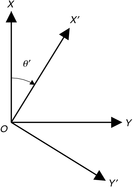
The MT tensor upon rotation of the horizontal axes
Upon rotation of the horizontal measuring axes clockwise by angle θʹ as shown in Figure 1, Equation 1 changes to
|

where


and so

or, more fully,

whence

and so

Thus the matrix [Zxx, Zxy; Zyx, Zyy] upon rotation of axes changes to [Zʹxx, Zʹxy; Zʹyx, Zʹyy] according to

of in-phase part

and quadrature part

Expanding Equation 21 shows that the elements of the two matrices Z and Zʹ are related by the equations


where

(taking the positive square root) and βp is defined by

It is also useful to define an angle μp as

and a (positive) quantity ZLp as

with an auxiliary angle βpʹ as

The angles βp, μp and βpʹ may all be determined with a range of 360°. Then

Note that (Zʹxxp + Zʹyyp), (Zʹxyp − Zʹyxp), Cp and ZLp are independent of θʹ, and so are ‘rotational invariants’.
Expanding Equation 22 in the same way as Equation 21 produces for the quadrature part of the tensor a set of equations just like 23 to 32, with subscript q replacing subscript p. Then (Zʹxxq + Zʹyyq), (Zʹxyq – Zyxq), Cq and ZLq are also seen to be independent of θʹ, and so also are rotational invariants.
The depiction of MT tensors using Mohr diagrams
The general case: 3D structure
It can be seen from Equations 23 and 24 that plotting Zʹxxp against Zʹxyp as the axes are rotated (i.e. θʹ varies) defines a circle, known (with its axes) as a Mohr diagram. An example is shown in Figure 2a, for the general case of 3D conductivity structure. For the in-phase case, the centre of the circle is at the point [(Zxyp – Zyxp)/2, (Zxxp + Zyyp)/2] and the radius of the circle is Cp. Different points on the diagram can be checked to confirm that Equations 23 to 32 for the rotation of axes are obeyed. Figure 2a further shows how axes for Zʹyxp and Zʹyyp may be included on the diagram, to display the variation of these components also.

|
Following the same procedure for the quadrature part of an MT tensor produces a similar Mohr diagram, and diagrams for in-phase and quadrature data may be presented as adjacent figures. Such pairs are shown in Figure 2b, c, which also draws attention to the particular cases of 2D and 1D conductivity structure to which the 3D case simplifies.
When axes for Zʹyxp and Zʹyyp are included it is clear to see why the phase of Zxy (as the arctangent of the ratio Zxyq/Zxyp of two evidently positive quantities Zxyq and Zxyp) is commonly in the range 0° to 90°, and the phase of Zyx (as the arctangent of the ratio Zyxq/Zyxp of two evidently negative quantities Zyxq and Zyxp) is commonly in the range 180° to 270° (or equivalently –180° to –90°).
2D structure
When the geologic structure is 2D and the axes are rotated to be along and across geologic strike, the rotated MT tensor will have the form [0, Zν; –Zχ, 0] where it is expected that all of Zνp, Zνq, Zχp and Zχq will be positive.
At that rotation the terms Zʹxxp and Zʹyyp in Equations 23 and 26 are both then zero. This circumstance produces two demands, firstly that

with the consequence that the centre of the Mohr circle lies on the Zʹxyp axis, and secondly that

For non-zero Cp there are thus two solutions for θʹ, notably

i.e.

There is thus an ambiguity of 90° in the determination of angle θʹ, which (see Figure 1) is now the strike angle, relative to the initial observing axes.
The same procedure as described so far in this section may be followed for the quadrature part of an MT tensor, to produce a set of equations like Equations 33 to 36 with subscript p replaced by subscript q. Then as shown in Figure 2b, the diagram becomes a pair of circles with origins on the Zʹxyp and Zʹxyq axes; angles μp and μq are zero. Because for 2D the in-phase and quadrature strike directions are the same,

and the in-phase and quadrature radial arms are parallel.
Zν and Zχ are described as the TE and TM (or vice-versa) modes of 2D induction, where TE stands for ‘transverse electric’ and TM stands for ‘transverse magnetic’. These modes are also sometimes called E–pol and B–pol respectively, for ‘E-polarisation’ and ‘B-polarisation’.
1D structure
If a 2D case simplifies further to become a 1D case, then Zν = Zχ = Z say, and the tensor for all rotations has the form [0, Z; –Z, 0], where Zp and Zq are both positive. With reference to Equations 24 and 25, the terms Zʹxyp and Zʹyxp must be constant for varying θʹ, demanding that

Because the lengths of the two radial arms thus vanish, the diagram reduces to a pair of points on the horizontal axes, as shown in Figure 2c.
‘Singularity’ of a tensor
A tensor is said to be singular when it has a determinant of zero, and cannot be inverted (Strang, 2003). Mohr diagrams display this situation clearly: when the determinant is zero, the circle will go through the origin of axes (in Figure 2a, ZL = C). With a further construction which may be added to Figure 2a, a Mohr diagram also shows the determinant quantitatively (Lilley, 2016: 96).
As can be seen from inspection of Figure 2 generally, it is possible for 3D and 2D cases to be singular, but not 1D cases. The condition of singularity may be thought of as the extreme limit of anisotropy in a tensor (whether 2D or 3D).
Application of a matrix method similar to SVD
Where as Equations 13, 17 and 20 involve rotating the E and H axes together, the reduction of the observed tensor to a 2D form may be achieved by rotating the E and H axes separately. The rotations are by angles θep and θhp respectively for the in-phase part of the tensor, and by angles θeq and θhq respectively for the quadrature part of the tensor. Each procedure is very similar to traditional singular value decomposition (Strang, 2003), but in both cases the relevant 2 × 2 matrix is anti-diagonalised, rather than diagonalised.
Thus, taking the H field to be completely in-phase, solutions are sought for

and

where it is instructive to compare the form of these equations with Equation 17.
Equation 39 may be expressed as

and Equation 40 expressed as

From Equation 41 the in-phase part of the tensor, Zp, is factored into

and from Equation 42 the quadrature part is factored into

Again, it is instructive to compare Equations 43 and 44 with Equation 20.
The four components of Equation 43 may now be solved for the four unknown quantities θep, θhp, Υp and Ψp to yield:


and

Similarly Equation 44 may be solved to give an equivalent set of solutions for the quadrature part of a tensor: the quantities θeq, θhq, Υq and Ψq are given by Equations 45, 46, 47 and 48 with subscript p replaced by subscript q. The quantities Υp, Υq, Ψp and Ψq are here termed ‘principal values’.
Note that Equations 29, 45 and 46 give

and Equations 28, 45 and 46 give

Equations 30, 45, 46 and 48 give

and Equations 27, 45, 46 and 47 give

The quantities μp, βp, ZLp and Cp in Figure 2 are thus related to the quantities which arise in the SVD analysis, and a Mohr diagram is seen to also display the SVD results of the present section.
An example which illustrates this point and uses the equivalent notations is shown in Figure 3. The figure has been drawn for the tensor (with all real components)

|

The values of θep, θhp, Υp and Ψp evaluated by Equations 45 to 48 above are 31.7°, 21.4°, 8.09 and 3.09 respectively. As a tutorial exercise, these values may also be read graphically off the figure.
While the use of Equations 45 to 48 should be straightforward to determine the quantities θep, θhp, Υp and Ψp (and similarly θeq, θhq, Υq and Ψq) it is possible also to use a standard SVD algorithm, and adapt the results to give the desired quantities. Lilley (2012) discusses the results given if a matrix such as that of Equation 53 is put into a standard SVD computing routine.
Thus by rotation of the electric and magnetic axes separately, the example MT tensor has been reduced to an ideal 2D form. This exercise may be regarded as a standard SVD but adjusted to anti-diagonalise, rather than diagonalise the matrix.
In a search for the nearest 2D model in a 3D situation the results thus obtained may be valuable to bear in mind. On the grounds that distortion occurs in the electric field rather than the magnetic field, the rotated magnetic axes may give a useful indication of an ‘approximate 2D regional strike’. The rotated electric axes may show a dominant direction of electric field distortion.
Invariants of rotation
Many of the quantities arising so far are invariant with the rotation of the observing axes. In Figure 4 it is shown how, by inspection, an MT tensor can be expressed in terms of seven such invariants. This figure shows two figures of the form of Figure 2a juxtaposed, the left-hand one for the in-phase MT data, and the right-hand one for the quadrature MT data. Clearly λp, μp and ZLp are independent of λq, μq and ZLq, to the extent that the in-phase and quadrature parts of an MT tensor are determined independently. Also all of λp, μp, ZLp, λq, μq and ZLq are independent of θʹ, and so are invariants of axes rotation.

|
The seventh invariant shown, δβ, can be seen to also be independent of θʹ because as θʹ changes the radial arms of both circles rotate together. The angle between the two radial arms (δβ) is constant and thus is also an invariant of rotation. In this paper, δβ is defined as

There are a number of different practical invariants in MT (Berdichevsky and Dimitriev, 1976; Ingham, 1988; Szarka and Menvielle, 1997; Weaver et al., 2000). The use of such invariants for dimensionality analysis has been developed especially by Marti et al. (2005, 2009, 2010) and Marti (2014); see also Jones (2012). This paper will focus on the seven invariants shown in Figure 4 and others closely related to them, and discuss the useful information they convey. Thus the eight elements of an MT tensor, all of which generally change upon axes rotation, are expressed as seven invariants of rotation plus just one quantity which does vary as the axes are rotated. As an example of the latter, the angle β in Figure 2a defines the ‘observed point’, and the tensor element values at this point in turn respond to the directions of the measuring axes.
The set of invariants given in Figure 4 will now be reviewed.
Two invariants summarising the 1D character of the tensor
The two invariants ZLp and ZLq summarising the 1D character are straightforward and were termed ‘central impedances’ by Lilley (1993). For graphical representation it may be convenient to multiply them by T1/2, in view of the common tendency of tensor elements to show a period dependency of T–1/2 (see Units of E, Z and H).
Alternatively they may be combined as per Equations 10 and 11 and presented as values of apparent resistivity (ρa ZL) and phase (φZL), computed as

and

An example of this presentation will be given below in Figure 9.
Two invariants summarising the 2D character of the tensor
Two invariants λp and λq measure the 2D character of the MT tensor, and are also straightforward. They are naturally angles, and were termed anisotropy angles by Lilley (1993). With reference also to Figure 2a they may be expressed

and

where λp and λq are both in the range 0 to 90°. Note this definition fails if either Cp > ZLp or Cq > ZLq (or both), and the relevant circle encloses its origin of axes.
The special cases λp = 0 and λq = 0 arise when the data show nil 2D characteristics. The data are then either pure 1D; or ‘twisted 1D’ (Lilley, 1993), and so 3D.
The special cases λp = 90° and λq = 90° arise when the in-phase and quadrature parts respectively of the tensor are so anisotropic as to be singular. Thus a value of λp and λq near 90° indicates that a condition of singularity is being approached.
Two (of three) invariants summarising the 3D character of the tensor
The two angles μp and μq shown in Figure 4 characterise the 3D nature of the impedance tensor and are also straightforward. It may be useful to express them as their mean and difference values (this practice is adopted in the example below) because certain mechanisms for causing 3D effects, notably those with a strong twist component, give similar μ contributions to both the in-phase and quadrature parts of a tensor (Lilley, 1993). In cases of the distortion of a regional 2D structure by a ‘twist’ factor only, the twist is then measured by (μp + μq)/2 and the difference (μq – μp) should be zero.
The third 3D invariant: the ‘7th invariant’
The third 3D invariant shown in Figure 4, δβ, can be seen to be the angle by which the two radial arms of the in-phase and quadrature circles are not parallel. It is significant as of the invariants shown in Figure 4, it alone links the in-phase and quadrature parts of an observed tensor. Care must be taken with its sign (see Equation 54). This ‘7th invariant’ and other invariants closely related to it will be discussed further below.
The invariants of Bahr (1988) and Weaver et al. (2000)
This paper will shortly introduce a 7th invariant which is developed from the δβ of Figure 4, and is used below in place of the 7th invariant of Weaver et al. (2000). As context, it is necessary to first summarise both the analysis of Bahr (1988), and also the ‘WAL2000’ analysis of Weaver et al. (2000). The reason is that the 7th invariant of WAL2000 is closely linked to the Bahr analysis.
The Bahr (1988) analysis
In this important and pioneering model of tensor distortion, Bahr first notes that if a regional 2D tensor with an unknown (but defined) strike is distorted by a (purely in-phase) tensor d according to

where Z2D has the form [0, Zν; –Zχ, 0], then

when the measuring axes are aligned with the regional strike.
When, as in the general case, the measuring axes are not aligned with the regional strike, there will be an angle α for measuring-axes rotation at which a magnetic signal in the Hʹx direction will give an electric field signal  which is linearly polarised. At that rotation, the measuring axes will be aligned with the regional strike.
That is, the phases of Zʹxx Hʹx and Zʹyx Hʹx must be the same, and so the phases of Zʹxx and Zʹyx must be the same. Thus

and Equation 61 can be used to find a solution for α. In fact two solutions for α will be found, and in the (ideal) case of Equation 59 they will differ by 90°.
However values of rotation angle α which give the ‘equal phase’ condition of Equation 61 can be sought for any observed MT tensor. Call two such solutions α1 and α2, and in this paper both are defined in the range 0 ≤ α < 180°, with α2 > α1.
For the ideal case of Equation 59 the two α values differ by 90°. Thus the closer the difference between the two α values now found is to 90°, the closer the actual MT situation is to the ideal model. At best, two such values found for α will give the direction of a 2D regional geologic strike (with a 90° ambiguity).
Bahr (1988, 1991) further defines a ‘phase-sensitive’ skew value η as an ‘ad hoc’ measure of the departure from his model of data being fitted to it. Such values for η are included in the example of MT data given below. For the mathematical derivation of η the interested reader is referred to the papers cited, and see also Simpson and Bahr (2005). For an η value of zero the regional structure is indeed 2D, the data conform to Equation 59, and again the strike is given, with a 90° ambiguity, by either α1 or α2 (which now differ by 90° exactly).
In the general case where the equal-phase condition of Equation 61 is met for axes rotation α1, an angular deviation ξ1 of the telluric field in the yʹ direction occurs such that

and also

Similarly for axes rotation α2, with correspondingly different values of [Zʹxx, Zʹxy; Zʹyx, Zʹyy], an angular deviation ξ2 occurs such that

and also

The Bahr analysis can be displayed on a Mohr diagram, as shown in Figure 5 for the example data NQ101R at period T = 0.0353 s. At this period, two solutions for α have indeed been found (α1 = 46.1° and α2 = 139.9°). The upper part of Figure 5 is reproduced in Appendix A in more detail. It can be seen that (π – α2 + α1) is indeed close to 90°, and thus α2 is indeed close to (α1 + 90°).

|
For many MT data, however, solutions for α1 and α2 will not be found, consistent with a condition given by Bahr (1988) not being met. For the example data presented below, as the graphs there will show, only for parts of the data spectrum is the condition satisfied and angles α1 and α2 found.
The set I1, I2, I3, I4, I5, I6 and I7 of Weaver et al. (2000)
The first six of the set of invariants of Weaver et al. (2000) follow the set of invariants of Lilley (1998) and comprise the ZLp, ZLq, λp, λq, μp and μq of Figure 4, with the changes that sines of angles are taken rather than the angles themselves. Thus ZLp is taken as I1 and ZLq is taken as I2, but sin λp (rather than λp) is taken as I3, and sin λq (rather than λq) is taken as I4.
Further, rather than taking μp and μq individually, their sum (μp + μq) and difference (μq – μp) are taken. Then, again taking sines rather than basic angle values, WAL2000 define sin(μp + μq) as I5 and sin(μq – μp) as I6.
Taking the sines of angles is intended to produce values with magnitudes on the convenient scale of 0 to 1, but this procedure does not allow for angles greater than 90° without introducing ambiguity in interpretation, because sin(π – μ) = sinμ. While the values of λp and λq will never exceed 90°, in cases of strong distortion the values of μp and μq may exceed 45° so that the value of (μp + μq) may indeed exceed 90°. Cases of such strong distortion are not uncommon, and thus the use of actual angle values (rather than taking their sines) is followed generally in the present paper.
The seventh invariant of WAL2000, denoted I7, is not the obvious δβ from Figure 5, but rather is based on the ideal galvanic distortion model of Bahr. In terms of the Bahr model described above, the WAL2000 I7 has the value

and may be demonstrated graphically by a construction added to Figure 5, as discussed in Appendix A below.
Weaver et al. (2000) also show that their I7 is related to δβ (using the notation of Figure 4 of the present paper) by

where the dimensionless quantity Q (also an invariant) is defined as

Values of I7 may thus be calculated using Equation 67 even when solutions for α1 and α2 do not exist and Equation 66 cannot be applied. Such values of I7 calculated using Equation 67 are included in the section below, but note they are susceptible to instability when Q, the denominator of Equation 67, becomes small. Also, once solutions for α1 and α2 can no longer be found, the appeal of I7 as being simply related to α1 and α2 is lost and the physical significance of I7 becomes obscure. This situation gives rise to further enquiry regarding possible ‘7th’ invariants.
Appendix B presents some further notes on the resolution of the slightly different definitions for the Bahr strike angles of the Bahr (1988) and Weaver et al. (2000) papers.
Invariant Δβ, an extension of δβ
As illustrated by Figures 3 and 4, Equations 50 and 54 give

which in view of Equation 49 may be expressed

Thus, for the simplest cases where θeq = θep, the angle δβ in Figure 4 will take the value of (μq – μp), and the value of (μq – μp – δβ) will be zero.
A further invariant is thus suggested, here called Δβ and defined as

which tests whether (μq – μp – δβ) is indeed zero. When not zero, Δβ gives a measure of the departure of the observed tensor from the situation in which all 3D characteristics are accounted for by the quantities (μq – μp) and (μp + μq)/2, and so more basically by μp and μq.
Note further that Δβ is the angle which occurs in the cosine factor in Equation 68. Also, that by Equations 70 and 71, Δβ can be expressed in the simple form:

It is a condition of 2D cases that θeq = θep, (see Figures 2 and 3). Thus Δβ = 0 is the case automatically in all 2D cases, whether or not the anisotropy is strong.
But note that Δβ will also become small and approach zero in 3D cases where there is a strongly dominant direction of electric field signal, for which θeq ≈ θep. This situation may occur in 3D cases where, for example, the MT tensor approaches singularity in both its in-phase and quadrature parts, due to strong distortion by a pure-real tensor.
For completeness it should be added that, for 1D cases, θep and θeq do not exist (see Figures 2 and 3), and Δβ is not defined.
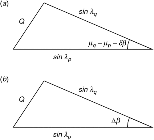
Δβ and Q
Equation 68 for Q may be displayed as the geometric relationship shown in Figure 6. In Figure 6b, the angle Δβ is now seen to have a major influence in controlling the magnitude of Q. It is evident that Q has the range 0 ≤ Q ≤ 2, and that to minimise Q the value of (μq – μp – δβ) must be zero. Study of Figure 6 makes clear the further condition required for Q = 0, that λp = λq.
|
The condition Q = 0 thus requires that both the in-phase and the quadrature parts of an MT tensor have the same 2D measure, i.e. that λp = λq, and also the same 3D measures, i.e. that μq – μp = 0. The condition Q = 0 further requires that βq – βp = 0. The condition Q = 0 is thus met only by one particular and highly restricted class of 3D (and 2D) structures, though note that there is a special case possible for Q = 0 in which (μq – μp) – (βq – βp)= 0 but μq – μp ≠ 0 and βq – βp ≠ 0, with λp = λq.
The quantity Q is thus comprehensive in being a function of both the 2D and the 3D measures of an MT tensor. However it is just this very property, of showing a combined 2D and 3D response, that causes Q to be a less appropriate ‘7th’ invariant than Δβ. Non-zero values of Δβ are a function of 3D characteristics only.
Some further invariants
This section describes a number of further invariants, which will be compared for the characteristics they show in the analysis of field data.
Invariants (λp + λq)/2 and (λq – λp)
As noted in the section Two invariants summarising the 2D character of the tensor, the quantities λp and λq are both gauges of two-dimensionality. In the next section below they are presented as mean and difference values, following the practice developed for μ values.
Invariants det Zp and det Zq
The determinants of the in-phase and quadrature parts of the MT tensor taken separately, given by

and

are invariants, and reduce to zero if Zp and Zq respectively approach conditions of singularity (Lilley, 2016: 96). They are included in the example results below multiplied by period T (and so as det Zp T and det Zq T) to counter the common T–1/2 period dependency of tensor element values, explained in the section Units of E, Z and H.
Invariants κp and κq
The quantities κp and κq are condition numbers, as defined for magnetotelluric data by Lilley (2012). In Figure 3, κp is given by

and will become large as the in-phase part of the tensor approaches the condition of singularity (and its Mohr circle approaches the origin of axes). κq is defined, and behaves, similarly.
Dimensionless and invariant with axes rotation, κp and κq are thus direct gauges of the in-phase and quadrature parts respectively of a tensor approaching singularity. Because they are ratios they do not depend on the absolute values of the tensor elements, as do the invariants det Zp and det Zq.
Examples using MT data: the site ‘NQ101R’
The invariants described above are now presented graphically for data from a particular Australian MT site, NQ101R, which is offered as typical of many sites. Analysis begins with the NQ101R data as tensor-element values in the practical units of mV/km/nanotesla. In the graphs in the present section, the unit of apparent resistivity is Ωm, and the unit for angles (including phase) is degree. The NQ101R data set has been chosen as, over the period range of observation, its characteristics change greatly, though not in an atypical way. Results for just one observing site are thus sufficient to show a wide range of significant 2D and 3D characteristics.
Thus Figure 7 shows the basic MT data, supplied as in-phase and quadrature values at different periods of the elements of [Zxx, Zxy; Zyx, Zyy], and here presented as plots of apparent resistivity (in panels A1-A4) and phase (in panels B1-B4), taking each element separately (see Equations 10 and 11). It can be seen that the situation occurs where, with increasing period, ρa Zyy grows to be greater than ρa Zyx; and where as ρa Zxx gets very weak, its phase goes ‘out of quadrant’, i.e. out of the expected range between 0° and 90°.

|
Panels A5 and B5 show the det Zp T and det Zq T determinant values reducing to near zero with increasing period, as both the in-phase and quadrature parts of the tensor approach singularity.In panels A6 and B6 the condition numbers, κp and κq, give different measures of the same phenomenon, now with values increasing above 10 as the in-phase and quadrature parts of the tensor approach singularity.
The panels C1 and D1 show Mohr diagram presentations of the observed data, and exhibit much of the information spelled out in the other panels.
The panels C3, D3, C4 and D4 show the singular value decomposition of the tensor as outlined in the section Application of a matrix method similar to SVD above, where the major principal values (in-phase and quadrature) have been combined to give ρa ZPyx (apparent resistivity) and φZPyx (phase) results, as have the minor principal values to give ρa ZPxy and φZPxy results. The rotation angles for the electric field axes, θep and θeq, are given in panels C5 and D5, and the rotation angles for the magnetic field axes, θhp and θhq, are given in panels C6 and D6. Over the whole period range the θe values (panels C5 and D5) are in good agreement, and change little. The θh values (panels C6 and D6) also are in good agreement, but are period dependent,changing through almost 90° over the period range.
On the grounds that distortion is in the electric field rather than in the magnetic field, one might look to both θhp and θhq as indicative of 2D strike. However the data are too 3D for a 2D model to be justified, a conclusion demonstrated particularly by the period dependence of the θhp and θhq results.
Figure 8 shows further invariants of the NQ101R data. Panel E1 shows the invariant I1 of WAL2000 as determined, and panel F1 shows I1 multiplied by T1/2 to counter the T–1/2 period dependency referred to above. Similarly panels G1 and H1 display I2 which, with I1, indicates the ‘1D magnitude’ of the data.

|
Panels E2 and F2 then show the two anisotropy angles λp and λq, which measure two-dimensionality. In panels G2 and H2 the means and differences of these two angles are plotted, showing that they are similar at the start and finish of the period range, but for mid-periods they differ substantially. At the start of the period range both λ values are at their minimum, and at their closest to one-dimensionality. At long periods, especially the λp values approach their limit of 90°.
In panels E3 and F3 the basic measures of three-dimensionality (relative ‘twist’) are displayed, and in G3 and H3 the means and differences of these quantities are given. Again note that from a 2D (or 1D) start, with both μ values effectively zero, the three-dimensionality increases with period, to ‘plateau’ at long periods (see panel G3). As in panel H2, in panel H3 the differences between in-phase and quadrature values are greatest at mid-periods.
Panel E4 presents δβ and panel F4 presents I7, the WAL2000 seventh invariant calculated using Equation 67. In exceeding the value of unity I7 transgresses the intention of the WAL invariants to have a magnitude in the range 0 – 1, and also it can clearly not be interpretated as the sine of an angle. Panel G4 displays the values of Q, and panel H4 the values of Δβ, to which attention is drawn below as being of particular interest.
Panels E5 and F5 display the Bahr α values where they exist.Panel G5 displays them combined to give a ‘mean strike direction’, and panel H5 presents the difference between the two strike direction estimates. Panel E6 gives the Bahr η values, and panel F6 the sine of the difference of the two strike directions (i.e. the sine of the values in panel H5). The values in panel F6 may thus be compared to the I7 values plotted in panel F4 above, and noted to agree where values for α1 and α2 exist. Panels G6 and H6 then give the Bahr ξ values, where they exist.
Finally in Figure 8 panels E7 and F7 present, as mean and difference values, the θep and θeq values from panels C5 and D5 of Figure 7. Consistent with Equation 72, in F7 the values taken by (θeq – θep) can be seen to be half those of Δβ as in panel H4 above. Panels G7 and H7 similarly present as mean and difference values the θhp and θhq values from panels C6 and D6 of Figure 7.
Remembering from Figure 6 the control of Q by the λp and λq values and by Δβ in particular, it can be seen in panel G4 that Q is indeed close to zero when (in panel H2) λq ≈ λp, and (in panel H4) Δβ ≈ 0.
Discussion
Observed MT data may thus be summarised as shown for NQ101R in Figure 9. The left-hand two columns present the tensor element data in their basic form, and the right-hand two columns present the data as values of seven invariants, Iʹ1 to Iʹ7:

|
-
in panel K1 the central-impedance apparent resistivity ρa ZL, here called Iʹ1;
-
in panel L1 the central-impedance phase φZL, here called Iʹ2;
-
in panel K2 the mean 2D anisotropy (λp + λq)/2, here called Iʹ3;
-
in panel L2 the 2D anisotropy difference (λq – λp), here called Iʹ4;
-
in panel K3 the mean 3D ‘twist’ (μp + μq)/2, here called Iʹ5;
-
in panel L3 the 3D ‘twist’ difference (μq – μp), here called Iʹ6; and
-
in panel K4 the 3D-sensitive Q-angle Δβ, here called Iʹ7 .
Panel L4 then completes the set with rotation-dependent quantity θhp, which under certain circumstances gives an indication of geologic strike. A rotation of the horizontal measuring axes at the observing site would cause all values of θhp to experience a zero shift. Also, from the infinite number of tensors which share the same seven invariants Iʹ1 to Iʹ7 (one tensor at every point around the circles in Figure 4), the rotation-dependent value θhp selects the original tensor. Picking up the point of Weidelt and Chave (2012: 129), the eight values (Iʹ1 to Iʹ7 and θhp) together allow the recovery of the original tensor in a straightforward way.
To now review Figure 9, at the short-period end of the spectrum the data are 2D, with Iʹ5, Iʹ6 and Iʹ7 all near zero. In fact, to the extent that Iʹ3 and Iʹ4 are also both small, the data are approximately 1D, indicating near-surface apparent resistivity and phase values as given by Iʹ1 and Iʹ2 respectively.
As period lengthens, the data become both more 2D (as Iʹ3 increases), and more 3D (as Iʹ5 increases), with Iʹ4 and Iʹ6 giving information on the consistency (or otherwise) of these characteristics between the tensor in-phase and quadrature parts.
At the long-period end of the spectrum the data are now strongly 3D, even extremely so, indicated by the values of Iʹ3 approaching 90° with significant values of Iʹ5. The in-phase and quadrature parts of the tensor are in fact both approaching singularity, which is also shown by the long-period (red) circles in panels C1 and D1 of Figure 7 approaching their respective origins of axes.
A particular interest lies in the Iʹ7 values in panel K4, which for the long-period end of the spectrum remain small while the 2D and 3D indicators Iʹ3 and Iʹ5 steadily increase in value. The reason for this behaviour is that the increasing three-dimensionality in the data is of a particular type, in which there is a dominant electric field direction common to both parts of the MT tensor.
Conclusions
This paper has focussed on expressing an observed magnetotelluric tensor as a set of seven rotational invariants, together with a single quantity which is rotation dependent.Attention has been given to expressing the invariants diagrammatically, as an aid to understanding their behaviour and significance.
Results for an example observing site (NQ101R) demonstrate that it is straightforward to compute such invariants as a function of period. Particular characteristics of the dimensionality of the data are commonly then shown to be period-dependent.
Attention has focussed in this paper on a newly-recognised invariant Δβ which in the example shown is found, perhaps unexpectedly, to be near zero even when other indications of three-dimensionality are high. In the context of the complications possible in 3D geological structures, low Δβ values indicate a simplifying feature which may prove to be an aid in the interpretation and modelling of MT data.
Conflicts of interest
The author declares no conflicts of interest.
Acknowledgements
The author thanks John Weaver, Peter Milligan and Chris Phillips for valuable discussions over many years on the subject matter of this paper. The NQ101R data were provided by Geoscience Australia. Two anonymous reviewers are thanked for helpful comments, and Mark Lackie and Graham Heinson are thanked for editorial support.
References
Bahr, K., 1988, Interpretation of the magnetotelluric impedance tensor: regional induction and local telluric distortion: Journal of Geophysics, 62, 119–127.Bahr, K., 1991, Geological noise in magnetotelluric data: a classification of distortion types: Physics of the Earth and Planetary Interiors, 66, 24–38.
Berdichevsky, M. N., and Dimitriev, V. I., 1976, Basic principles of interpretation of magnetotelluric curves, in A. Adam, ed., Geoelectric and geothermal studies, KAPG geophysical monograph: Akademiai Kaido Budapest, 165–221.
Berdichevsky, M. N., and Dmitriev, V. I., 2008, Models and methods of magnetotellurics: Springer.
Caldwell, T. G., Bibby, H. M., and Brown, C., 2004, The magnetotelluric phase tensor: Geophysical Journal International, 158, 457–469.
Chave, A. D., and Jones, A. G., eds., 2012, The magnetotelluric method: theory and practice: Cambridge University Press.
Hobbs, B. A., 1992, Terminology and symbols for use in studies of electromagnetic induction in the Earth: Surveys in Geophysics, 13, 489–515.
Ingham, M. R., 1988, The use of invariant impedances in magnetotelluric interpretation: Geophysical Journal of the Royal Astronomical Society, 92, 165–169.
Jones, A. G., 2012, Distortion of magnetotelluric data: its identification and removal, in A. D. Chave, and A. G. Jones, eds., The magnetotelluric method: theory and practice: Cambridge University Press, 219–302.
Lilley, F. E. M., 1993, Magnetotelluric analysis using Mohr circles: Geophysics, 58, 1498–1506.
Lilley, F. E. M., 1998, Magnetotelluric tensor decomposition: Part I, Theory for a basic procedure: Geophysics, 63, 1885–1897.
Lilley, F. E. M., 2012, Magnetotelluric tensor decomposition: insights from linear algebra and Mohr diagrams, in H. S. Lim, ed., New achievements in geoscience: InTech Open Science, 81–106.
Lilley, F. E. M., 2016, The distortion tensor of magnetotellurics: a tutorial on some properties: Exploration Geophysics, 47, 85–99.
Marti, A., 2014, The role of electrical anisotropy in magnetotelluric responses: from modelling and dimensionality analysis to inversion and interpretation: Surveys in Geophysics, 35, 179–218.
Marti, A., Queralt, P., Jones, A. G., and Ledo, J., 2005, Improving Bahr’s invariant parameters using the WAL approach: Geophysical Journal International, 163, 38–41.
Marti, A., Queralt, P., and Ledo, J., 2009, WALDIM: a code for the dimensionality analysis of magnetotelluric data using the rotational invariants of the magnetotelluric tensor: Computers & Geosciences, 35, 2295–2303.
Marti, A., Queralt, P., Ledo, J., and Farquharson, C., 2010, Dimensionality imprint of electrical anisotropy in magnetotelluric responses: Physics of the Earth and Planetary Interiors, 182, 139–151.
Simpson, F., and Bahr, K., 2005, Practical magnetotellurics: Cambridge University Press.
Strang, G., 2003, Introduction to linear algebra (3rd edition): Wellesley–Cambridge Press.
Szarka, L., and Menvielle, M., 1997, Analysis of rotational invariants of the magnetotelluric impedance tensor: Geophysical Journal International, 129, 133–142.
Weaver, J. T., Agarwal, A. K., and Lilley, F. E. M., 2000, Characterization of the magnetotelluric tensor in terms of its invariants: Geophysical Journal International, 141, 321–336.
Weidelt, P., and Chave, A. D., 2012, The magnetotelluric response function, in A. D. Chave, and A. G. Jones, eds., The magnetotelluric method: theory and practice: Cambridge University Press, 122–164.
Young, H. D., and Freedman, R. A., 2016, University physics with modern physics (14th edition): Pearson Global.
Appendix A
Details of the Bahr analysis shown by a Mohr diagram
The axes rotation angles α1 and α2 introduced in the section The Bahr (1988) analysis and Figure 5 are shown in more detail in Figure A-1.

|
In an ideal Bahr case, (α1 + π – α2) will have the value 90°. It can be seen in Figure A-1, diametrically opposite the point marked with a star, that this condition is close to being satisfied in the present case. In such circumstances, where α1 and α2 both exist, the WAL2000 invariant I7 may be obtained from the departure of (α1 + π – α2) from 90°. Call this departure angle ε. Then


and the sine of the amplitude of ε is taken as I7.
Appendix B
Clarification of computations of the I7 of WAL2000
Using their notation, equations 48 and 49 of Weaver et al. (2000) are

and

where θ1 and θ2 are strike directions, θʹ is a ‘mean strike direction’, and d41 and d23 are calculated from values of an observed MT tensor. Using the relationship

Equations B-1 and B-2 become, respectively,

and

In turn these equations give

and

Subtracting Equation B-7 from Equation B-6 gives

and so

as in Weaver et al. (2000) with the implication that when I7 = 0, the equalities θ1 = θ2 = θʹ accompany galvanic distortion in a 2D region.
However note that for I7 = 0 Equation B-4 has the solution

and Equation B-5 has the solution

leading upon the addition of Equations B-10 and B-11 to

Then, rather than take θ1 = θ2 as in Weaver et al. (2000) it is clearer, as shown in Figure 5, to think of θ2 = θ1 + π/2 for galvanic distortion in a 2D region. That is, θ2 should not be thought of as departing from θ1 (and so equal to θ1 in an ideal situation), but as departing from θ1 + π/2 (and so equal to θ1 + π/2 in an ideal situation). By way of illustration, in Figure A-1 the angles α1 and α2 are not approximately the same, but are different by close to 90°.