

Quantifying the differences between gravity reduction techniques
Philip HeathGeological Survey of South Australia, 4/101 Grenfell Street, Adelaide, SA 5000, Australia.
Email: philip.heath@sa.gov.au
Exploration Geophysics 49(5) 735-743 https://doi.org/10.1071/EG17094
Submitted: 28 July 2017 Accepted: 5 October 2017 Published: 6 November 2017
Journal Compilation © ASEG 2017 Open Access CC BY-NC-ND
Abstract
Gravity data processing (reduction) generally utilises the best-available formulae. New and improved formulae have been introduced over time and the resulting newly processed gravity will not match the old. Additionally, mistakes made in the gravity reduction process, as well as the incompatibilities between various equations, will inevitably lead to errors in the final product. This can mean that overlapping gravity surveys are often incompatible, leading to incorrect geological interpretations. In this paper I demonstrate the magnitude of change that results when different information is introduced at various stages of the gravity reduction process. I have focussed on differences relating to calibration factors, time zones and time changes, height, geodetic datums, gravity datums and the equations involved therein. The differences range from below the level of detection (0.01 mGal) to over 16.0 mGal.
The results not only highlight the need to be diligent and thorough in processing gravity data, but also how it is necessary to document the steps taken when processing data. Without proper documentation, gravity surveys cannot be reprocessed should an error be identified.
Key words: error, geodesy, gravity, processing, reduction.
Introduction
A common product of Australian state and territory geological surveys is a regional Bouguer gravity map. These images are compilations of multiple gravity surveys and it is an ongoing problem that overlapping surveys rarely match. Most commonly there appears to be an offset between the surveys, leading to mismatched points and anomalies in the final image. Numerous attempts have been undertaken to create a smooth image of the gravity in South Australia using merging tools and different gridding algorithms (e.g. Heath et al., 2012), but to date a perfect image hasn’t been created.
There are multiple reasons that surveys might mismatch. Different resolutions from different gravity meters as well as different precision and accuracy in elevation measurement techniques are two common issues. Another issue is how the data are processed. The process of gravity reduction is straightforward; however, at each step of the process decisions need to be made regarding which formulae to use, which gravity and geodetic datum is required and so on. This paper attempts to quantify some of the differences involved in using different equations.
Multiple software packages exist (e.g. Intrepid Geophysics & Geosoft) that have the ability to process raw gravity data. In order to have full control over the reduction process I have constructed a simple spreadsheet to undertake reduction in the field or in the office with minimal effort and to avoid software licensing issues. (The spreadsheet has been tested by undertaking gravity reduction using similar software and comparing results. The approach has allowed me to analyse the differences involved at different stages of the gravity reduction process should erroneous information be input. It is freely available to anyone who requests it.)
Many geophysical textbooks contain information regarding the gravity reduction process (e.g. Blakely, 1995; Parasnis, 1962; Telford et al., 1990); however, these don’t contain comparisons between what happens when equations of different vintage are used. Talwani (1998) discusses the errors involved in Bouguer reduction, especially relating to the gravity effect of a spherical cap and Bullard B correction, which I have not replicated here.
A series of examples have been undertaken to illustrate quantitatively how much difference is introduced at various stages of the gravity reduction process. Each demonstration takes an element of the process, inserts realistic, but incorrect, values and presents the results in a series of tables.
Method and results
Applying the scale factor
The scale factor (often referred to as a Calibration Factor; Heath, 2016) is a multiplication factor that must be applied to all raw gravity readings. A typical Scintrex CG5 gravity meter measures relative gravity values in mGal; however, the dynamic range of the meter doesn’t match reality. As an illustrative example, two points on the Earth’s surface with the values 980 000 and 980 100 mGal, respectively, have a difference of 100 mGal. In comparison, a gravity meter might measure 4000 and 4100.1 mGal with a difference of 100.1 mGal. Therefore, a scaling factor must be calculated before all survey work by recording values at the end points of a calibration range with a significant change (typically over 50 mGal) in the gravity values. The scale factor (c) is the ratio of the actual difference in gravity (Δga) to the measured difference in gravity (Δgm):

Raw gravity readings must be divided by the scale factor c. One potential source of error is using the inverse of the calibration factor (effectively multiplying instead of dividing by c). For a typical scale factor of 0.9997281, a typical raw reading of 3785.98 mGal becomes 3787.01 mGal if applied correctly and 3784.95 mGal if the inverse is used, creating a difference of 2.06 mGal. The dynamic range of a Scintrex CG5 is 1000 to 9000 mGal, meaning this error could range from anywhere between 0.5 to 5.0 mGal (for the scale factor referred to here).
Methods to calculate c
For the simplest approach, c can be calculated from two measurements on the calibration range. It can also be calculated from an ABABA-type loop between two points A and B. In both cases the processor must decide to assume either a linear drift in the measurements, or to undertake a more thorough calculation to determine the scale factor. Furthermore, the processor may have multiple readings to choose from. If a CG5 is being used, does the processor choose the readings with the lowest standard deviation (s.d.) or should they average them all? A single measurement on a CG5 gravity meter is actually an average of a series of readings; hence, s.d. is available for each measurement. The following demonstration shows the effects of computing different scale factors from the same set of observations.
Table 1 shows the raw data collected from a gravity calibration run between the Kensington Gardens Sportsfield and Norton Summit Cemetery, South Australia.

|
Eight scenarios are considered, each a different way to calculate the calibration factor. The scenarios are:
-
Scale factor using two ‘best’ values only (from first A and B readings);
-
Scale factor using two average values (from first A and B readings);
-
Scale factor using average values, assuming linear drift (from first ABA loop);
-
Scale factor using average values, assuming linear drift (from second ABA loop);
-
Scale factor using average values, assuming linear drift (ABABA);
-
Scale factor using best values only, treated as a gravity loop (from first ABA loop);
-
Scale factor using best values only, treated as a gravity loop (from second ABA loop); and
-
Scale factor using best values only, treated as a gravity loop (ABABA).
For each calculation technique (listed 1 to 8 above) I’ve calculated the scale factor and the minimum and maximum corrected value of a CG5 gravity meter, assuming a dynamic range of 1000 to 9000 mGal. I’ve then calculated the difference between the values calculated from each scenario with the final scenario (which is arguably the most accurate). The differences range from 0.01 to ~1.00 mGal. Table 2 shows these results.

|
Scenario 3 produces the least difference compared to Scenario 8. Scenario 4 is effectively the same as Scenario 3, as it uses the same method, just at a different time. Most of the scenarios produce a maximum difference in the range of 0.1 to 0.2 mGal, with the greatest difference (1.0 mGal) resulting from Scenario 2, where only two values are used to calculate the scale factor.
To illustrate how different scale factors affect a gravity survey, consider the Coompana gravity survey (Allpike, 2017). The dynamic range of the survey is –64.59 to 19.20 mGal, a total of ~84 mGal. This survey used three CG5 gravity meters, one measuring at ~2500 mGals, one at 4000 mGals and one at 5000 mGals. I’ll call these gravity meters 1, 2 and 3, respectively, and I designate each gravity meter with its own scale factor from the scenarios above. I assign gravity meter 1 the scale factor from scenario 2, gravity meter 2 the scale factor from scenario 5, and gravity meter 3 the scale factor from scenario 8. If gravity meter 1 measures values from 2458 to 2542 mGal (84 mGal around 2500 mGal), the scaled values become 2456.954–2540.921 mGal, a difference of 83.964 mGal. Performing the same operation for gravity meters 2 and 3, we find scaled values of 83.972 and 83.973 mGal, respectively. The maximum difference here is 0.009 mGal, just under the 0.01 mGal level of detection.
Scale factor gravity datum
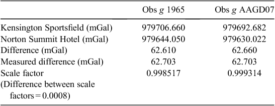
The scale factor will also be different depending on the gravity datum used for the known values in the calculation. Assuming the difference recorded on a CG5 meter is roughly the same, the difference in the scale factor is noticeable. Table 3 illustrates this, and further examples can be found in Hackney (2001), chapter 5.
|
The average of the scale factor differences in Table 2 is 0.05 mGal. Using a CG5 gravity meter, a measured difference between the two points is 62.703 mGal (this is a separate loop from the one shown in Table 1). The resulting difference in the two scale factors (using the two differences in Table 3) is 0.0008. Over the dynamic range of a CG5, this will lead to differences between 0.8 and 7.2 mGal. The maximum differences in the scale factors used in the Coompana example is ~0.0001, eight times smaller than the difference here.
Finally, it is worth noting that scale factor values change over time due to spring changes and other instrument factors. The two values below were calculated using the same method (method 8 above) and gravity meter on two dates approximately four months apart, and they differ by 0.000139785682:


Over the dynamic range of a CG5, changes in scale factor values over time will result in differences of 0.14 to 1.26 mGal. Although it is unlikely the measurement range of a single gravity meter will change enough over the course of four months to affect the magnitude of readings, these results suggest that a scale factor should be undertaken before all surveys.
It’s worth noting that the scale factors presented here can be reduced to seven significant figures without affecting the magnitude of the final difference.
Effect of time on gravity reading
The equation that determines the observed gravity (in the Australian Absolute Gravity Datum 2007 (AAGD07)) from raw readings can be written as Equation 2:

where b07 is the known base station value (in AAGD07), c is the scale factor from Equation 1, r1 is the first reading at the base station, rs is the reading taken at the station, rf is the final reading at the base station, t1 is the time of the first reading at the base station, ts is the time of the reading at the station and tf is the time of the reading at the final base station. For gravity datums other than AAGD07, simply change the datum of the known base station value b07.
Two ways in which time can affect the value given by Equation 2 are if the wrong number is inserted for a time due to operator error (e.g. setting the wrong UTM zone or not setting daylight savings time on the CG5) or through processing error (e.g. typing the wrong number into the reduction software).
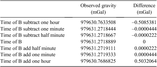
If, for example, we assume the error is due to processing, this can be demonstrated by taking the simple gravity loop shown in Table 1 and modifying the time component.
Consider the raw CG5 data in Table 4. Given the known value at A (Kensington Sportsfield) is 979706.660 mGal, the reduced value of B (Norton Summit Cemetary; subtracting one minute) is 979631.272 mGal (Table 5). The results of altering the time of B by adding and subtracting half-minutes, whole minutes and whole hours are shown in Table 5. While this isn’t a comprehensive list of all possible gravity values, it should be suffice to demonstrate that the difference is negligible (< 0.01 mGal) for small time changes.

|
|
The time of a gravity measurement is typically recorded to the nearest minute. A reading on a CG5 gravity meter is effectively an average of a series of measurements, so the time recorded on the internal computer is the average time of the measurements to a precision of the nearest second. Changes of an hour due to incorrectly setting daylight savings time on a gravity meter can also be tested by simply modifying the time.
If the time zone (or latitude) is set incorrectly on a CG5 and the CG5 has been set up to calculate the tidal correction, a further correction will need to be applied. The incorrect tidal correction will need to be removed and the correct one added. Numerous webpages are available that can calculate tidal corrections (for no charge) for any part of the world, at any time, and are ideal for applying these corrections. Tidal corrections are cyclical, vary between ~–0.1 and ~0.1 mGal and have a wavelength of ~12 h.
Hackney (2001) illustrates distinct improvement in gravity reference network misclosures when instrument tide corrections were removed and recalculated using the more accurate latitude of the station in question.
Height and gravity
A simple experiment to show the effect of height on gravity can be conducted by measuring acceleration due to gravity from on top of and underneath a desk. This experiment was undertaken at the Geological Survey of South Australia offices. We found that for a difference in height of 72 cm, the change in gravity was ~0.30 mGal (Figure 1). Linear extrapolation of the results shown in Figure 1 indicate that for over 1 m in height the change in gravity is ~0.42 mGal.

|
Each time a gravity meter is placed on a tripod and levelled, the sensor will be at a different height above the ground. This height can be measured, recorded and added to the elevation as measured by Differential GPS. For regional surveys, this might be added as a constant throughout the survey (~24 cm when using a CG5), but for microgravity surveys (measuring to tens of microgals (Sheriff, 1991) the elevation must be carefully taken into account. This can be demonstrated from some sampled survey data. Consider the data presented in Table 6. This data is from a portion of a microgravity survey undertaken in early 2017 (Heath et al., 2017). The table shows the station numbers, observed gravity readings, heights, Bouguer gravity values and the difference between Bouguer gravity values for three stations. The three readings selected show a range of sensor heights from 21 to 28.2 cm, and the difference in Bouguer gravity ranges from 0.041 to 0.055 mGal, detectable on the CG5 gravity meter. A microgravity survey such as in Heath et al. (2017) may be looking at gravity anomalies with magnitudes smaller than 0.26 mGal, suggesting this height measurement is important for precise Bouguer gravity values.

|
The effect of using an incorrect height in processing can also be demonstrated by taking an existing loop, modifying the height of a single point and observing the differences. Considering again the loop shown in Table 4, Table 7 shows the same reading repeated 14 times but with incorrect heights. The final two columns are simple Bouguer anomalies and the difference between the actual values. These are consistent with the calculations in the desk experiment (Figure 1) and the microgravity example (Table 6). The difference becomes noticeable when the height varies more than ~5 cm.

|
Another potential difference in height comes when using Orthometric heights instead of Ellipsoidal heights in the Bouguer calculation. Until recently, it has been routine to use Orthometric heights in gravity calculations as they represent a height from an equi-gravity datum (i.e. sea level, see Reynolds, 1997). However, this thinking has fallen out of favour as Hackney and Featherstone (2003) and Hinze et al. (2005) explain. Not using the Ellipsoidal height leads to under- or over-correction of normal gravity (theoretical gravity) when computing free-air or Bouguer anomalies. The difference between Elliposidal and Orthometric heights is generally in the order of meters, so the differences in gravity value will be greater than in the height examples shown in Tables 6 and 7. This issue is particularly relevant when comparing older, pre-GPS surveys with newer surveys, as normal/theoretical gravity is always linked to a particular ellipsoid and free-air/Bouguer anomalies are always relative to the surface of that ellipsoid. And, of course, in the past we didn’t have a good way to determine Ellipsoidal heights, which leads to issues when merging older datasets with newer ones.
Gravity datums
The fifth demonstration relates to gravity datums. The Geological Survey of South Australia commonly use three gravity datums: Isogal65 (Potsdam), Isogal84 (ISGN1971) and AAGD07. To add further confusion, these are often presented in different units: either mGal or μms–2.
There are two commonly used equations to convert between Isogal65 and Isogal84 in Australia (Wellman et al., 1985):


where
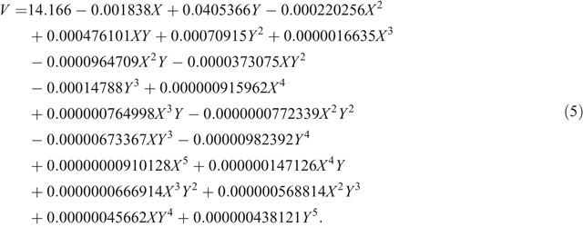
In Equation 5, X is the longitude minus 135° east and Y is the latitude minus 25° south (i.e. if using the equations, use a positive value of latitude in the southern hemisphere).
The difference between Isogal65 and Isogal84 values is ~14 mGal; however, the difference varies depending on which equation is used. For a point in Adelaide, the Isogal65 value is 979 706.660 mGal, giving Isogal84 values of 979 692.811 mGal (using Equation 3) and 979 692.237 mGal (using Equation 4). The difference between the values is 0.574 mGal. Generally this isn’t a problem unless converting values back and forth between datums, in which case a single formula should be used only. These issues occur in databases such as the South Australian geophysical database (SA Geodata) and Geoscience Australia’s Geophysical Archive Data Delivery (GADDS) system, which use different equations to automatically populate whichever values are not present in the database.
The following equation is used to convert between Isogal84 and AAGD07 (in mGal):

Another issue between datums occurs when published values don’t match. Consider the data in Table 8. The gravity values for De Rose Hill in South Australia, for example, are 978975.48 mGal (Isogal65) and 9789612.42 μms–2 (AAGD07). Using Equations 3 to 6 to convert between the values results in differences of 0.07 or 0.08 mGal.The highest variation found in South Australia was at the Meningie Homestead Woolshed, with a difference of 0.55 mGal.A comprehensive analysis of all Isogal stations in Australia is beyond the scope of this paper, but should be examined.

|
Theoretical gravity
The sixth demonstration relates to theoretical gravity. The latitude of the gravity measurement is part of the theoretical gravity correction component of gravity reduction. Telford et al. (1990) give the theoretical gravity equation for the GRS1967 ellipsoid; however, different sources provide slightly different equations (see list below). There are newer equations for GRS80 and WGS84 as well as the older 1930 equation. Some of these are listed here:

(Sheriff, 1991; Blakely, 1995; Reynolds, 1997)


(Telford et al., 1990; Reynolds, 1997)


(Wikipedia (https://en.wikipedia.org/wiki/Theoretical_gravity); Hackney and Featherstone, 2003; Hinze et al., 2005)


(Wikipedia, https://en.wikipedia.org/wiki/Theoretical_gravity)


(modified from Sheriff, 1991)
Equations 7 to 12 use a simplified form of what is represented in the ‘closed form’ of Equations 13 to 17. This simplification was initially used due to limited computational power. Equation 16 is as presented in Sheriff (1991); it appears to be a misprint and Equation 17 here is a modified version of the equation.
Table 9 demonstrates the differences from Equations 7 to 17. I’ve taken a series of Australian latitudes (–10° to –45°) and calculated the theoretical gravity for each using Equations 7 to 17. I’ve then subtracted each value from selected ‘benchmark’ equations (those with the most references) to demonstrate the difference between 1967 and 1984 values. Typically, the 1930 equation (Equation 7) is different by ~16 mGal, the 1967 equations differ up to ~1 mGal, the 1984 equations differ up to ~0.14 mGa, and the difference between 1967 and 1984 values is in the order of 0.8 mGal.

|
The seventh demonstration illustrates what happens when latitudes in a different geographic datum are used in the theoretical gravity calculation. Using AGD66 instead of GDA94 values (or vice versa) in the theoretical gravity equation will yield different values.
To demonstrate the difference in theoretical gravity between AGD66 and GDA94 values, I’ve taken a range of Australian AGD66 latitudes (–10° to –45°) and calculated the equivalent GDA94 values as well various theoretical gravity values at these points. Table 10 shows the gravity values, and Table 11 shows the differences (up to ~1.0 mGal).

|

|
The eighth demonstration illustrates how all these issues feed into the final Bouguer anomaly. These arise as combinations of all the previously described scenarios.
To demonstrate a combination of errors in calculating the Bouguer anomaly: if an incorrect datum is used in a calculation (error 0.83 mGal), the elevation is out by 20 cm (error 0.4 mGal) and an incorrect calibration number is used (error 1 mGal). In other words, the total isn’t simply the sum of these errors. To demonstrate, consider again the simple loop in Table 4. The difference in the observed gravity is 0.5297 mGal and the difference in the Bouguer anomaly is –0.3667 mGal, as shown in Table 12.

|
Finally, it’s worth mentioning hysteresis effects in Scintrex CG series gravity meters. The hysteresis effect occurs as the result of spring relaxation following transport of the gravity meter between stations, and not necessarily over rough terrain. It usually manifests itself as a slow increase or decrease in readings over half an hour or more once the instrument is levelled at a station. This is evident in the readings in Table 1. The average increase between first and last reading (over 5 min) is ~0.023 mGal. This is a significant amount and raises the question of which value to use for a given station where multiple measurements are recorded. This is not usually documented in gravity acquisition reports. For a thorough analysis of the hysteresis effect on a CG-3M gravity meter see Repanić and Kuhar (2017).
Discussion
Geophysicists at the Geological Survey of South Australia have tried for many years to produce a ‘perfect’ image of the state gravity. This has involved experimenting with different gridding techniques: grid merging (Heath et al., 2012), levelling (Heath and Katona, 2016) and supervised variable density gridding (Heath and Katona, 2016; Katona, 2017).
In exploring these techniques it became apparent that simply flagging surveys that didn’t fit well and not using them as part of the gridding process was the quickest way to handle them. This isn’t a complete solution, and is potentially removing information that would otherwise be useful in a state grid product. This paper is an exploration of the reasons why surveys undertaken in the same area may not match.
As is apparent, there are many reasons why surveys in the same area may not match. Trying to correct for these inconsistencies can be difficult, as the information needed is not always available. Some of the information can be determined by back-calculation (e.g. if you have a Bouguer anomaly value, ellipsoid elevation, density and observed gravity it should be possible to determine which theoretical gravity equation was used) but some information can’t easily be recovered (e.g. if only a station number and Bouguer anomaly are provided).
There are many other potential sources of error in gravity surveying (not least of all potential confusion arising from the terms Isogal65, AGD66 and GRS67). Some of the operation errors include (when using a CG5 instrument) setting the internal clock incorrectly and incorrectly setting the reference point on the meter. Other sources of error involve terrain corrections and atmospheric corrections. There are far too many sources of error to include in this paper, so I’ve restricted myself to those commonly involved in the processing of data.
Thorough documentation and staff training are essential for a successful gravity survey. I argue that a successful survey be undertaken by well-trained staff, and documentation contain (at a minimum) enough information to calculate the Bouguer anomaly from the raw readings during each step of the process.
Conclusions
Inconsistencies in processing gravity data can lead to errors in the final product. I’ve demonstrated that errors due to calibration factors, time zones, height, geodetic datum, gravity datum and the equations used all lead to an incorrect value for gravity at a point. These errors, combined with other potential sources of error not discussed here, mean that adjacent or overlapping gravity surveys will often not correlate.
As new geodetic models will undoubtedly be created from time to time, it would be naïve to set some sort of standard; rather, I suggest that all gravity surveys should be documented to a level where the observed and Bouguer gravity anomalies can be recreated from raw readings. This transparency in gravity processing will allow gravity surveys to be reprocessed should any issues with the survey be found and should ultimately allow better gravity products.
The largest source of error discussed in this paper is the effect of using an incorrect theoretical gravity equation (Equation 16). Ignoring the ‘incorrect’ equation and using the 1930 equation (Equation 7), when the 1984 equation (Equation 14) would be more appropriate, leads to an error of over 16 mGal.
Conflicts of interest
The author declares no conflicts of interest.
References
Allpike, R., 2017, Coompana gravity survey: Atlas Geophysics Report Number R2017051, Atlas Geophysics.Blakely, R. J., 1995, Potential theory in gravity and magnetic applications: Cambridge University Press.
Hackney, R. I., 2001, A gravity-based study of the Pilbara-Yilgarn Proterozoic Continental Collision Zone and the South-Eastern Hamersley Province, Western Australia: Ph.D. thesis, The University of Western Australia.
Hackney, R. I., and Featherstone, W. E., 2003, Geodetic versus geophysical perspectives of the ‘gravity anomaly’: Geophysical Journal International, 154, 35–43
| Geodetic versus geophysical perspectives of the ‘gravity anomaly’:Crossref | GoogleScholarGoogle Scholar |
Heath, P., 2016, Quantifying the errors in gravity reduction: ASEG-PESA-AIG 2016, 25th International Geophysical Conference and Exhibition, Extended Abstracts, 582–588.
Heath, P., and Katona, L., 2016, Gravity gridding in South Australia: ASEG-PESA-AIG 2016, 25th International Geophysical Conference and Exhibition, Extended Abstracts, 720–722.
Heath, P., Reed, G., Dhu, T., Keeping, T., and Katona, L., 2012, Regional terrain corrected gravity grid production: examples from South Australia: Preview, 156, 120
Heath, P., Gouthas, G., Irvine, J., Krapf, C., and Dutch, R., 2017, Microgravity surveys to identify potential hidden cavities on the Nullarbor: Report Book 2017/00021. Department of the Premier and Cabinet, South Australia, Adelaide.
Hinze, W. J., Aiken, C., Brozena, J., Coakley, B., Dater, D., Flanagan, G., Forsberg, R., Hildenbrand, T., Keller, G. R., Kellogg, J., Kucks, R., Li, X., Mainville, A., Morin, R., Pilkington, M., Plouff, D., Ravat, D., Roman, D., Urrutia-Fucugauchi, J., Veronneau, M., Webring, M., and Winester, D., 2005, New standards for reducing gravity data: the North American gravity database: Geophysics, 70, J25–J32
| New standards for reducing gravity data: the North American gravity database:Crossref | GoogleScholarGoogle Scholar |
Katona, L., 2017, Gridding of South Australian ground gravity data, using the Supervised Variable Density Method: Report Book 2017/00012. Department of the Premier and Cabinet, South Australia, Adelaide.
Kearey, P., Brooks, M., and Hill, I., 1984, An introduction to geophysical exploration (3rd edition): Blackwell Publishing.
Parasnis, D. S., 1962, Principles of applied geophysics: Chapman and Hall.
Repanić, M., and Kuhar, M., 2017, Modelling hysteresis effect in Scintrex CG-3M gravity readings: Geophysical Prospecting, ,
| Modelling hysteresis effect in Scintrex CG-3M gravity readings:Crossref | GoogleScholarGoogle Scholar |
Reynolds, J. M., 1997, An introduction to applied and environmental geophysics: John Wiley & Sons.
Sheriff, R. E., 1991, Encyclopedic dictionary of applied geophysics (4th edition): The Society of Exploration Geophysicists.
Talwani, M., 1998, Errors in the total Bouguer reduction: Geophysics, 63, 1125–1130
| Errors in the total Bouguer reduction:Crossref | GoogleScholarGoogle Scholar |
Telford, W. M., Geldart, L. P., and Sheriff, R. E., 1990, Applied geophysics (2nd edition): Cambridge University Press.
Wellman, P., Barlow, B.C., and Murray, A.S., 1985, Gravity base-station network values, Australia (report 261): Bureau of Mineral Resources, Geology & Geophysics.