Development and numerical tests of a Bayesian approach to inferring shallow velocity structures using microtremor arrays
Ikuo Cho 1 4 Takaki Iwata 2 31 Geological Survey of Japan, AIST, 1-1-1 Higashi, Tsukuba, Ibaraki 305-8567, Japan.
2 College of Community Development, Tokiwa University, 1-430-1 Miwa, Mito, Ibaraki 310-8585, Japan.
3 Institute of Statistical Mathematics, 10-3 Midori-cho, Tachikawa, Tokyo 190-8562, Japan.
4 Corresponding author. Email: ikuo-chou@aist.go.jp
Exploration Geophysics 49(6) 881-890 https://doi.org/10.1071/EG18011
Submitted: 17 January 2018 Accepted: 19 January 2018 Published: 19 March 2018
Journal compilation © ASEG 2018 Open Access CC BY-NC-ND
Abstract
We propose an empirical Bayesian approach to inferring shallow (depth ranges from a few to several tens of metres) S-wave velocity structures using microtremor arrays and execute numerical tests to assess the feasibility of this approach. In our approach, the estimate of the S-wave structure (posterior) is derived from an empirical S-wave structure model (prior) and phase velocities of Rayleigh waves obtained with microtremor arrays. In other words, we aim to find a model that is close to the empirical model and is able to explain phase velocities with a 1D surface-wave theory. The inversion is stabilised by the constraints from the prior model so that model parameterisation with many thin layers can be adopted. The velocity structure is individually estimated for each of two cases (assumptions): the case where we assume fundamental-mode dominance and the case where we take into account the higher modes. Optimal values of the model parameters (e.g. a thickness parameter) are found, based on Akaike’s Bayesian Information Criterion (ABIC), and the choice of the better assumption of the surface-wave theory is also based on ABIC. Numerical tests, where synthetic data is generated from a horizontally stratified two-layer model, indicate that the relative weight between a prior model and the observed data is appropriately adjusted by ABIC. It is revealed that a value of the thickness parameter required to reproduce the given two-layer model is successfully found by ABIC. We also suggest that we can make a plausible choice of the assumption of the surface-wave theory with ABIC, unless observation error is extremely large.
Key words: arrays, inversion, modelling, passive, shallow, surface wave, velocity.
Introduction
Microtremor array surveys are a non-destructive method for the exploration of S-wave velocity structures that does not require artificial sources (Okada, 2003). Therefore, as microtremor array surveys for shallow velocity structures need only small-size arrays, they can be conducted very flexibly. They can be a tool to acquire data before attempting other exploration methods (e.g. Cho et al., 2013; Cho and Senna, 2016). However, despite its flexibility in the field, the data processing procedure (i.e. inversion to find a velocity structure) can be further improved.
The Society of Exploration Geophysicists of Japan Standardisation Committee (2008) generally recommends using three to several layers for an inversion model so as to keep the number of unknowns as small as possible in microtremor array analyses (e.g. Chimoto et al., 2016). In some studies, VS (S-wave velocity) is fixed and only the layer thickness is estimated (e.g. Goto et al., 2017). When we use a model with few layers or a model with a fixed velocity in each layer, however, it is difficult to identify singular features involving a low-velocity layer sandwiched between high-velocity layers or a high-velocity layer between low-velocity layers (structural singularity), which are often seen in shallow velocity structures.
One possible approach to inferring such a structural singularity is to make the thickness of each layer sufficiently thin and fixed at a certain value and to estimate the S-wave velocity for each layer. However, as the number of layers increases, the estimates generally become unstable (Cho et al., 1999). Although it may be possible to impose a smoothing constraint for stabilisation, the arbitrariness of the strength of such a constraint then becomes a problem (Fukahata, 2009). It is desirable to develop a flexible and objective method to capture the wide variability of shallow (several metres to several tens of metres in depth) velocity structures.
Another problem when inverting a velocity structure is an arbitrary choice of the assumption of a surface-wave theory for the forward calculation. We frequently assume that the fundamental-mode Rayleigh waves dominate the vertical motions of microtremors. This assumption seems quite common, in particular, for the spatial autocorrelation (SPAC) method (Aki, 1957), which has been widely adopted in recent years (e.g. Chimoto et al., 2016; Goto et al., 2017). However, higher modes are indeed easily excitable in shallow structures (e.g. landfills including remarkable velocity inversion and high-contrast structures such as an alluvial layer on basement rock). In general, the phase velocities of the higher modes are faster than those of the fundamental mode, so that the S-wave velocity will likely be overestimated if we assume the dominance of the fundamental mode mistakenly (i.e. when higher modes coexist in the real wavefield). Conversely, the S-wave velocity will likely be underestimated if we assume the coexistence of the higher modes mistakenly (i.e. when only the fundamental mode exists in reality). Thus, the arbitrary assumption of the type of wavefield of the microtremors has always been a matter of concern (e.g. Poggi et al., 2012).
In light of this, inversion methods where we take into consideration the higher modes have been proposed, although there are few examples of such studies (e.g. Arai and Tokimatsu, 2005; Ikeda et al., 2012). In such cases, however, we may suspect that higher modes are actually excited. This is because the excitation of each mode depends not only on the velocity structure but also on the oscillation source.
These problems can be dealt with using a Bayesian approach. With a Bayesian approach, we incorporate a priori knowledge and/or information as probability distributions of parameters (prior distributions) and combine them with observed data to estimate improved probability distributions of parameters (posterior distributions). Because the subjectivity of the prior distribution is a problem in a Bayesian approach, a method called ‘empirical Bayes’, in which we determine the prior distribution based on the data, is currently widely used to avoid the subjectivity. This method maximises the statistical measure called the ‘marginal likelihood’ and is known in geophysics as Akaike’s Bayesian Information Criterion (ABIC) (Akaike, 1980). Since Akaike (1980), inversion methods based on empirical Bayes have been applied to many geophysical problems (Ogata et al., 1991; Koketsu and Higashi, 1992; Sekiguchi et al., 2000; Cho et al., 2006; Fukahata and Wright, 2008; Iwata, 2013, 2014) and this approach therefore appears to be well established (Matsu’ura et al., 2007; Fukahata, 2009).
Since the selection of the number of unknowns is not an essential problem in this approach (see subsection ‘Information criterion’), it is possible to use a sufficiently large number of layers to express a complex velocity structure that may include some structural singularities. Therefore, we can apply multiple models with various numbers of layers (from a few to many) to inversions. Because the difference in the numbers of layers is represented as the difference in a prior distribution in a Bayesian framework, we can select the best number of layers with ABIC. In a similar manner, the more likely assumption about the microtremor wavefield can also be selected objectively with ABIC.
In this way, the empirical Bayes approach offers various advantages, but it has almost never been used in the field of microtremor array analyses. Therefore, it is important to summarise and report on the basic principles of such an idea. Accordingly, we have compiled the basic theory and evaluated its applicability by conducting numerical tests with a two-layer model where we assumed that we were surveying a shallow velocity structure with small-size seismic arrays. In the following section, ‘Method’, we give details of the proposed method. The ‘Numerical tests’ section reports numerical tests and their results, which are discussed in the ‘Discussion’ and are summarised in the ‘Conclusions’.
Method
Overview
The proposed method assumes that an S-wave velocity structure is to be estimated from the phase velocities of Rayleigh waves, which are obtained by applying the SPAC method (Aki, 1957) or the centreless circular array (CCA) method (Cho et al., 2004; Tada et al., 2007; Cho et al., 2013) to circular-array data of vertical-component microtremors. A theoretical phase-velocity dispersion curve is calculated with a surface-wave theory assuming a horizontally layered velocity structure. More specifically, Hisada’s algorithm (Hisada, 1994, 1995) is used for the calculation. When the influence of the higher modes is taken into account, the equivalent phase velocity is synthesised through the method of Tokimatsu et al. (1992), where the ‘equivalent phase velocity’ is referred to as ‘apparent phase velocity’ in their original paper.
Parameterisation of velocity structure
The layer thicknesses remain fixed during the inversion process. Each layer is made sufficiently thin, but the layer thickness is modelled such that the layer thickness gradually becomes greater with depth, to keep the calculation time reasonable. Concretely, the thickness thki (m) of the ith layer from the surface is given by:

where a and b are layer thickness parameters (constants). Density and P-wave velocities in each layer are derived from the S-wave velocity using the empirical law of Ludwig et al. (1970).
Velocity structure modelling by the simple profiling method
The simple profiling method (SPM) is a conventional and empirical method used to convert a Rayleigh-wave phase-velocity dispersion curve into an S-wave velocity structure (Heukelom and Foster, 1960; Ballard, 1964; Gazetas, 1982; Cuéllar, 1994; Society of Exploration Geophysicists of Japan Standardisation Committee, 2008; Pelekis and Athanasopoulos, 2011). It provides a rough but practical estimate. An SPM profile is expected to be a good prior model in the absence of pre-existing survey data.
In this study, an SPM profile is created by the following procedure. First, a relation between the frequency freq and the (equivalent) Rayleigh-wave phase velocity Vr (i.e. the dispersion curve) is converted into a dispersion curve with respect to wavelength L, via the relation between the frequency and the wavelength: freq = Vr/L. Next, using the empirical relationships of dep = L/3 and Vr = 0.92VS, where dep is the depth, the dispersion curve is converted into an S-wave velocity-depth profile. Different values of the conversion factors have been used in different studies, with the L-dep conversion factor ranging between 1/3 and 1/2 and the VS-Vr conversion factor ranging between 0.87 and 1.00 (see the literature referenced at the beginning of this subsection). The conversion factor values used here are based on Gazetas (1982) and the Society of Exploration Geophysicists of Japan Standardisation Committee (2008). The values of VS in the SPM profile thus obtained are then averaged in each layer defined with Equation 1. Hereinafter, the velocity model obtained in this way is called the SPM model.
Inversion
The SPM model above is used as a prior distribution in our Bayesian approach. Let Nd and Nx be the numbers of observed data and unknown parameters, respectively. First, the observed phase velocity d (Nd-dimensional vector) and the S-wave velocity model x (Nx-dimensional vector) are associated mutually by the following statistical model:

where σ2E is a covariance matrix and |·| represents a determinant. The superscript T represents the transpose. The scalar quantity σ2 is a scaling factor of variances and covariances for data. The function f(·) (Nd-dimensional vector) represents the theoretical Rayleigh-wave phase velocities, which are to be compared with the observed phase velocities.
A vector x0 represents a set of prior values of the unknown velocity model x (see subsection ‘Velocity structure modelling by the simple profiling method’). When the prior distribution for x is a multivariate normal distribution with means x0 and a covariance matrix (σ2/λ2)D, its probability density function is given by:

In this study, the covariance matrices σ2E and (σ2/λ2)D are diagonal matrices; the diagonal components of which are denoted by σ2di (i = 1,⋯, Nd) and σ2ai (i = 1,⋯, Nx), and the non-diagonal components of both matrices are zero. The relative variances of the observed data and the prior distribution  and
and  are supposed to be known, and their scaling factors σ2 and λ2 are supposed to be unknown. These parameters are related to each other by the following equation:

A maximum a posteriori (MAP) estimate is a typical estimate in a Bayesian approach. It is a set of parameter values that maximise the posterior distribution. In our case, the posterior distribution is expressed by the following equation:

where

The value of x (=  ), which minimises S(x) of Equation 6, is a MAP estimate.
If a value of λ2 is known, the MAP estimate is obtained with the Levenberg-Marquardt method (e.g. Press et al., 2007), which is a standard quasi-nonlinear (iterative) technique. However, the value of λ2 is unknown. Therefore, we first give several different values to λ2, and obtain different MAP estimates for each of these. Then, we select from these different estimates the best estimates and the optimal value of λ2 with an information criterion described below.
Information criterion
Akaike (1980) proposed ABIC, defined by the following equation, to be used for comparison among multiple Bayes models (Bayesian model comparison):

where the marginal likelihood is given by:

A model with a smaller ABIC value is considered to be a better one.
By substituting Equations 2 and 3 into Equation 8, applying a Laplace approximation (Tierney and Kadane, 1986) and imposing the condition ∂L/∂(σ2) = 0 for maximising L (σ2, λ2|d), we obtain:

and

where  is the value of λ2 that minimises the right-hand side of Equation 10, and the value of
  is determined in practice by a grid search. A is a Jacobian matrix (
 ).
).
The marginal likelihood corresponds to the probability (value of the probability distribution) that the data d is obtained when parameter x is randomly extracted from the prior distribution p (x; σ2, λ2) and when data d is generated from the probability distribution p (d|x; σ2). It is known that the number of unknown parameters does not affect the Bayesian model comparison based on the marginal likelihood and overfitting due to an excessive number of parameters can be avoided (e.g. MacKay, 1995). This is because, as shown in Equation 8, the marginal likelihood evaluates the probability of data d appearing with respect to the whole parameter space, not the probability with respect to a specific value of the parameter.
Equation 7 can be used for comparison among Bayes models with different hyperparameter values that characterise prior distributions and likelihood functions, as well as Bayes models with different assumptions (e.g. Kass and Raftery, 1995). In this study, Bayesian models for two cases (the case where we assume fundamental-mode dominance and the case where we take into account higher modes), with various values of layer thickness parameters a and b, are compared based on Equation 10. More specifically, since the number of combinations of layer thickness parameters is six, as described in the next section, the comparison is made for 12 (= 6 × 2) models.
Numerical tests
Method
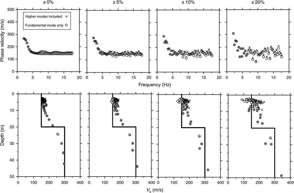
Two sets of theoretical phase velocities, which correspond to f(·) appearing in the subsection ‘Inversion’ are calculated: one for the case of the fundamental mode alone and one for the case where the higher modes are taken into account. A horizontally stratified two-layer velocity structure model (Figure 1 and Table 1) is used for both cases, where the upper layer with VS of 150 m/s has a thickness of 20 m, over a basement with VS of 300 m/s. The frequency range of the dispersion curve is from 2 to 18 Hz (sampled at a 0.36 Hz interval; Nd = 46). To mimic observation errors, fluctuations following a normal distribution N(0, s2) are given to the theoretical phase velocities. The resulting phase-velocity dispersion curve is called ‘synthetic data’ (phase velocity) or ‘observed data’ in this study. We consider four cases where the standard deviation s is set to 0%, 5%, 10% and 20% of the theoretical values. Therefore, 8 (= 4 × 2) dispersion curves of synthetic phase velocities are created. Hereinafter, the four synthetic datasets with the fundamental mode alone are called ‘synthetic data F’, and the other four synthetic datasets in which the higher modes are taken into account comprise ‘synthetic data M’.

|
Using these synthetic datasets, velocity structures are estimated. Estimation (inversion) is carried out with layer thickness parameter a fixed at 0.2, and six values of 1, 2, 5, 10, 20 and 30 are given as b. We consider two cases for the inversion: calculations of estimated values when assuming fundamental-mode dominance and when taking into account higher modes. These are called ‘analysis F’ and ‘analysis M’, respectively.
For each inversion, it is necessary to set the hyperparameter λ2 to a fixed value. Accordingly, inversion is carried out for the eight values of λ2 = 10−4, 10−3, 10−2, 10−1, 100, 101, 102, 103, and a search is made for λ2 that minimises the right-hand side of Equation 10. Therefore, 96 (= 6 × 2 × 8) inversions are carried out with different sets of parameter b and λ2 for each of the eight synthetic datasets.
In this study, the value of 1/3 is used for the L-dep conversion factor in the creation of the SPM model, but as mentioned above, different values of the conversion factor have been suggested in earlier studies, which tend to extend the deeper end of a model. Accordingly, at the deeper end of the inversion model, some layers are added until the depth of the midpoint of the lowermost layer reaches the maximum depth that is shallower than half the maximum wavelength. As a result, the depth of the upper surface of the lowermost layer ranges from 30 to 59 m, depending on the layer thickness parameter b. The number of layers NL ranges from 2 to 15.
Additionally, in order to take into account the stabilisation of the calculation, VS in the lowermost layer is fixed to the maximum value from the SPM data, and VS of the other layers is estimated. Therefore, the number of unknowns is NL – 1, which is equal to Nx. The standard deviations of the observed data and the prior distributions are assumed to be proportional to their respective average values, and 10% is given for  and
and  . These assigned standard deviations are merely provisional, and appropriate values of σdi and σai are estimated via the estimation of the scaling factors σ2 and λ2 (see Equation 4).
Based on the inversion results, differences in the marginal likelihoods given by different sets of the parameters b and λ2 are examined. The goodness-of-fit between the theoretical and the observed phase velocities and the reproducibility of the assumed velocity structure model are evaluated, respectively, by:

and

VSinv (depi) is the S-wave velocity of a velocity structure model obtained through the inversion procedure (hereafter referred to as an inverted model) at the ith depth depi, and VSgiven (depi) is the corresponding S-wave velocity for generating the synthetic data (true velocity structure model, hereafter referred to as the given model) (Figure 1 and Table 1). Ndep is the number of S-wave velocity sampling points (sampling depth) depi. We set dep1 and depNdep to 5 and 30 m, and Ndep to 251, respectively (i.e. the sampling is performed at every 0.1 m in the range from 5 to 30 m of depth).
We also examine whether the assumption (fundamental mode only or taking into account the higher modes) used in the creation of the synthetic data can be selected correctly with ABIC. If ABIC is smaller when analysis M (F) is applied to synthetic data M (F) than when analysis F (M) is applied, then ABIC is useful as a measure for judging whether analysis F or analysis M is more likely for a particular observed dataset.
Analysis results
Selection of hyperparameter λ2 and the number of layers
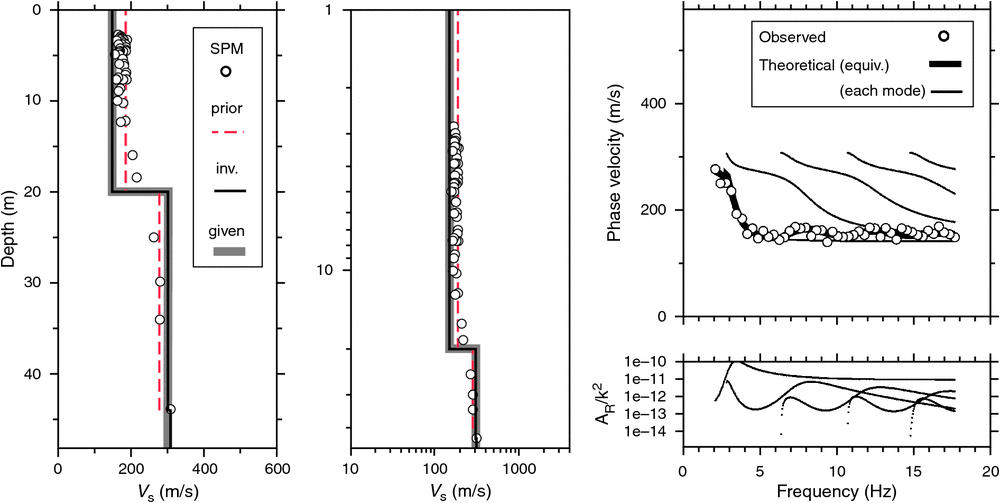
Figures 2–4 show inversion results for synthetic data M and s = 5% with analysis M. Figure 2 shows the case where b = 20 and λ2 = 0.01. The SPM velocity profile, prior model, inverted model and given model are plotted together in the left panel. The same are shown in the central panel in a logarithmic scale. The panel on the top right shows dispersion curves for the observed phase velocity (synthetic data), the theoretical equivalent phase velocity where we take into account the influence of the higher modes, and the phase velocity of each mode. The panel on the bottom right shows the medium response factors divided by the squared wavenumber as the weighting factors of each mode. In this case, it can be seen in Figure 3 that both the goodness-of-fit and reproducibility are satisfactory with RMSpv = 0.44 and RMSvs = 0.004, respectively. In addition, the deviation between the inverted and the prior models is small, and thus, an SPM gives an appropriate prior distribution.
|
|
Figure 3 shows six inverted models with different layer thickness parameter b. In each of the six panels, the model with the smallest ABIC among the cases with eight different values of λ2 is shown. The number of layers increases as b becomes small, and consequently, the change in VS with depth becomes smooth in general. This is because the SPM model that is given as the prior distribution (red broken line) approaches the raw SPM profile (open circles) and thereby becomes smoother with smaller b. Nonetheless, the velocity discontinuity at the depth of 20 m in the given model is reproduced to some extent in every profile, except for b = 30, indicating that the discontinuity at a depth of 20 m is an important factor in explaining the observed data.
The ABIC optimally strikes a balance between the fit of the inverted model to the prior model and the fit of the theoretical phase velocity to the observed data; the ABIC shows that the balance for the case with b = 20 is the best among the six inverted models (see ABIC values in each panel of Figure 3). As a matter of fact, every result shows an excellent fit to the observed data (i.e. RMSpv ranges from 0.44 to 0.52), except for the model of b = 30. The given model is reproduced as well, and RMSvs takes a value in the range from 0.004 to 0.19.
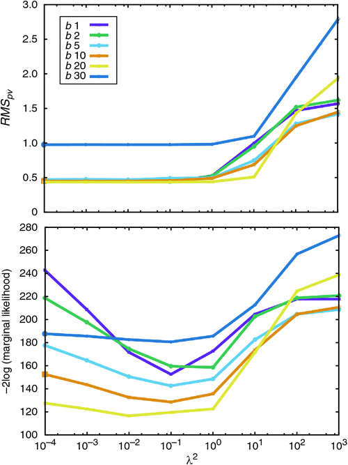
Figure 4 shows the change in RMSpv and (–2) × (log marginal likelihood) when b and λ2 are varied. Excluding the case of b = 30 where the first layer is too thick, every case shows a similar tendency. That is, while RMSpv generally takes an almost constant small value at λ2 < 1, it rapidly increases at λ2 > 1. Within the range of λ2 where RMSpv is almost constant, (–2) × (log marginal likelihood) finds a minimum value. This suggests that, through ABIC for each value of b, the optimal value of λ2 is found for which the deviation from the prior distribution is reduced while keeping the value of RMSpv small.
All five cases where the value of b ranges from 1 to 20 give a small RMSpv of the same degree when λ2 < 1. Therefore, the model in which the difference between x0 and x is the smallest for 1 ≤ b ≤ 20 is selected (see also Equation 6). As a result, the case of b = 20 is selected.
In this case, RMSvs is 0.004, which is by far the smallest in the five cases. This result, whereby a model that reproduces the true velocity structure well is chosen by the selection of layer thickness parameter b on the basis of ABIC, indicates that the proposed approach works appropriately.
Selection of the assumption about the wavefield
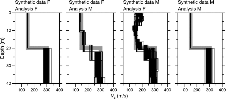
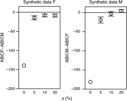
The left panel of Figure 5 shows the difference in ABICs when analysis F and analysis M are applied to synthetic data F, where a value of ABIC in Equation 10 is evaluated in each individual case of either analysis F or analysis M. Meanwhile, the right panel shows the difference in ABICs when analysis M and analysis F are applied to synthetic data M. To observe the significance of the results, the mean and standard deviation of the differences of 100 trials with assigning random fluctuations corresponding to observation errors are shown for each of s = 5%, 10% and 20%.
|
The left panel of Figure 5 reveals that ABICs by analysis M are larger than ABICs by analysis F for synthetic data F. That is, when the synthetic data are created using the model in which the fundamental mode is dominant (i.e. synthetic data F), the inversion analyses where we assume the dominance of the fundamental mode (i.e. analysis F) are accordingly evaluated as better Bayes models. Further, except for the case of s = 20%, the right panel shows the tendency for ABICs by analysis F to be larger than ABICs by analysis M for synthetic data M. That is, the inversion analysis in which the wavefield assumption agrees with that used in creating data is evaluated as a better case, except for the case with the largest observation errors.
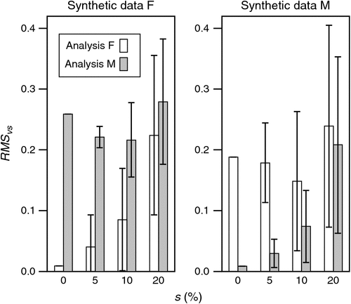
As shown above, from a viewpoint of statistical model comparison, the choice of the assumption about the wavefield is significant. It is true, of course, that the choice is unimportant if an inverted model does not depend on the choice. However, in our results, an inverted model (i.e. the reproducibility of the velocity structure) showed the dependency. More specifically, when the assumption about the wavefield was valid, RMSvs (the reproducibility of the velocity structure) generally remained at a few to 10%, but it did not fall below 10% when the wavefield assumption was not valid (except for the case of s = 20% in Figure 6). As the observation error got smaller, the difference became larger.
|
In order to visualise those differences in RMSvs, the variation of the velocity structure with different assumptions is compared in Figure 7. For example, for synthetic data F, analysis F (leftmost in Figure 7) reproduces the true velocity structure better than the analysis M (second from the left in Figure 7).
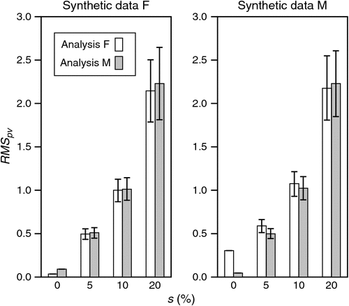
While such a difference appears in the reproducibility of the velocity model, there is no significant difference in RMSpv, the goodness-of-fit between the theoretical and observed phase velocities (Figure 8). RMSpv is comparable whichever assumption on the wavefield is used in the inversion procedures for all cases except s = 0%. This may be because as the observation errors in the dispersion curve become large, they conceal the influence of the higher modes.
|
The results above show the importance of the choice of assumption about the wavefield, not only for an interpretation of the wavefield, but also from the viewpoint of the accurate estimation of a velocity structure. They also show that the assumption cannot be selected correctly based on the goodness-of-fit between the theoretical and observed phase velocities (RMSpv) alone. Thus, we can say that the assumption is selected successfully with ABIC, and this indicates the effectiveness of the Bayesian approach in this study.
Discussion
The layer thickness parameter
Subsection ‘Selection of hyperparameter λ2 and the number of layers’ showed that the model with b = 20, for which the boundary depth at 20 m is the same as the given model, is selected as the best. This was regarded as evidence for the justification of the proposed method. However, one may think this is not a fair comparison, since the boundary depths in the given model and the models used in the inversion do not match except for the model with b = 20. Therefore, here, in addition to the case we have examined above, a numerical test is applied to the case of a = 0. In this case, since the layer thickness of the model is uniform regardless of depth, the models with b = 1, 2, 5, 10 and 20 commonly have a layer boundary at a depth of 20 m, similar to the given model.
The same numerical test for synthetic M and s = 5% with analysis M as in the subsection ‘Selection of hyperparameter λ2 and the number of layers’ was carried out in order to examine whether the model with b = 20 is still selected as the best. As a result, it was confirmed that the model with b = 20 was successfully selected.
It is worth noting that, from a statistical viewpoint, the proposed method can select not only the value of b but also a. If we think that the parameterisation for layer thickness does not appropriately reflect the real velocity structure, even though both variations of a and b are examined, we can modify Equation 1 and can assess whether Equation 1 or the modified equation is better.
Positioning of the proposed method and future tasks
In a conventional microtremor array survey, the number of layers is decided based on the experience and intuition of an expert so that the phase-velocity data can be explained by an inverted model with as few layers as possible (e.g. the Society of Exploration Geophysicists of Japan Standardisation Committee, 2008). It must also be decided whether the dispersion curve is influenced by higher modes or not. An expert will probably make appropriate decisions, but neither the criteria nor the reproducibility of his or her decisions is necessarily clear. This research has introduced a method for carrying out these decisions objectively, which is therefore applicable to automatic processing. A system that can obtain large amounts of data by small-size seismic arrays has been developed (Cho and Senna, 2016), and subsequently, for example, Wakai et al. (2017) carried out observations with small-size arrays at ~10 000 sites on the Kanto plain (as of February 2017). With such a background, there is great significance in enabling the substitution of expert decisions with automatic processing.
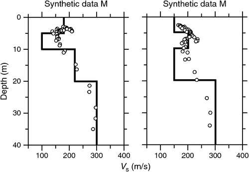
The proposed method can stably handle models with a relatively large number of layers (see subsection ‘Information criterion’). In addition, an SPM often reproduces features of a structural singularity. Therefore, the proposed method has the potential to be used as a tool for exploring such a structural singularity, which is often observed in shallow velocity distributions. For example, in Figure 9, a velocity model with a localised low-velocity anomaly or a localised high-velocity anomaly at a depth of 5 to 10 m is plotted together with the corresponding SPM profile. It can be seen that the SPM profiles roughly trace these structural singularities. As long as the SPM profile reproduces the features of complex soil structures in this way, our Bayesian approach is expected to reproduce those features with a resolution comparable to that obtained with an SPM. An examination of such potential is a future task.
|
Conclusions
This paper showed that an empirical Bayes approach with ABIC is effective in estimating a shallow (several metres to several tens of metres) S-wave velocity structure for a microtremor array survey. To evaluate feasibility, numerical tests were carried out. The proposed method adopts an S-wave velocity profile obtained with a simple conversion of the dispersion curve of phase velocity as a prior distribution. Then it evaluates, based on ABIC, the validity of the optimum layer thickness parameter (which also relates to the number of layers) and the assumption on the mode dominance in the microtremor wavefield. In the numerical tests, a horizontally stratified two-layer velocity structure model was used to generate synthetic data. It was demonstrated that the appropriate layer thickness parameter is selected. The numerical tests also indicated that ABIC is an appropriate measure to compare the validity of the two cases: the case where we assume the fundamental-mode dominance and the case where we take into account the higher modes.
Focusing on the presentation of the basic principle, we introduced the basic theory of the proposed method and reported on simple numerical tests as described above. The feasibility used with observed field data is for future work.
Conflicts of interest
The authors declare no conflicts of interest.
Acknowledgements
The authors thank the two anonymous reviewers for their useful comments that improved the original manuscript. The computer code used in this study was developed based on a downloadable code of Professor Yoshiaki Hisada. Fruitful discussions with Dr Toshiyuki Yokota helped the development of the program. The Generic Mapping Tools were used to generate the majority of the figures. This research was financially supported in part by the Japan Society for the Promotion of Science (JSPS) KAKENHI Grant Numbers JP15H04080, JP17K18962, and JP26241010.
References
Akaike, H., 1980, Likelihood and Bayes procedure, in J. M. Bernard, M. H. De Groot, D. U. Lindley, and A. F. M. Smith, eds., Bayesian statistics: University Press, Valencia, Spain, 143–203.Aki, K., 1957, Space and time spectra of stationary stochastic waves, with special reference to microtremors: Bulletin of the Earthquake Research Institute, University of Tokyo, 35, 415–457
Arai, H., and Tokimatsu, K., 2005, S-wave velocity profiling by joint inversion of microtremor dispersion curve and Horizontal-to-Vertical (H/V) spectrum: Bulletin of the Seismological Society of America, 95, 1766–1778
| S-wave velocity profiling by joint inversion of microtremor dispersion curve and Horizontal-to-Vertical (H/V) spectrum:Crossref | GoogleScholarGoogle Scholar |
Ballard, R. F., Jr, 1964, Determination of soil shear moduli at depths by in-situ vibratory techniques: Misc. Pap. No. 4–691, U.S. Army Engineer Waterways Experiment Station, Vicksburg, Miss.
Chimoto, K., Yamanaka, H., Tsuno, S., Miyake, H., and Yamada, N., 2016, Estimation of shallow S-wave velocity structure using microtremor array exploration at temporary strong motion observation stations for aftershocks of the 2016 Kumamoto earthquake: Earth, Planets, and Space, 68, 206
| Estimation of shallow S-wave velocity structure using microtremor array exploration at temporary strong motion observation stations for aftershocks of the 2016 Kumamoto earthquake:Crossref | GoogleScholarGoogle Scholar |
Cho, I., and Senna, S., 2016, Constructing a system to explore shallow velocity structures using a miniature microtremor array: accumulating and utilizing large microtremor database: Synthesiology, 9, 86–96
| Constructing a system to explore shallow velocity structures using a miniature microtremor array: accumulating and utilizing large microtremor database:Crossref | GoogleScholarGoogle Scholar |
Cho, I., Nakanishi, I., Ling, S., and Okada, H., 1999, Application of forking genetic algorithm fGA to an exploration method using microtremors: Butsuri Tansa, 52, 227–246
Cho, I., Tada, T., and Shinozaki, Y., 2004, A new method to determine phase velocities of Rayleigh waves from microseisms: Geophysics, 69, 1535–1551
| A new method to determine phase velocities of Rayleigh waves from microseisms:Crossref | GoogleScholarGoogle Scholar |
Cho, I., Tsurugi, M., Kagawa, T., and Iwata, T., 2006, Modelling of deep sedimentary velocity structure for evaluation of broadband strong ground motions: site-amplification spectra in Osaka sedimentary basin: Journal of Japan Association for Earthquake Engineering, 6, 113–132
| Modelling of deep sedimentary velocity structure for evaluation of broadband strong ground motions: site-amplification spectra in Osaka sedimentary basin:Crossref | GoogleScholarGoogle Scholar |
Cho, I., Senna, S., and Fujiwara, H., 2013, Miniature array analysis of microtremors: Geophysics, 78, KS13–KS23
| Miniature array analysis of microtremors:Crossref | GoogleScholarGoogle Scholar |
Cuéllar, V., 1994, Determination of the dynamic behaviour of soils using surface waves: Spanish experiences: Proceedings of the 10th World Conference on Earthquake Engineering, Balkema, Rotterdam, 6725–6734.
Fukahata, Y., 2009, Development of study of inversion analyses using ABIC in seismology: Zisin, 61, S103–S113
| Development of study of inversion analyses using ABIC in seismology:Crossref | GoogleScholarGoogle Scholar |
Fukahata, Y., and Wright, T. J., 2008, A non-linear geodetic data inversion using ABIC for slip distribution on a fault with an unknown dip angle: Geophysical Journal International, 173, 353–364
| A non-linear geodetic data inversion using ABIC for slip distribution on a fault with an unknown dip angle:Crossref | GoogleScholarGoogle Scholar |
Gazetas, G., 1982, Vibrational characteristics of soil deposits with variable wave velocity: International Journal for Numerical and Analytical Methods in Geomechanics, 6, 1–20
| Vibrational characteristics of soil deposits with variable wave velocity:Crossref | GoogleScholarGoogle Scholar |
Goto, H., Mitsunaga, H., Inatani, M., Iiyama, K., Hada, K., Ikeda, K., Takaya, T., Kimura, S., Akiyama, R., Sawada, S., and Morikawa, H., 2017, Shallow subsurface structure estimated from dense aftershock records and microtremor observation in Furukawa district, Miyagi, Japan: Exploration Geophysics, 48, 16–27
| Shallow subsurface structure estimated from dense aftershock records and microtremor observation in Furukawa district, Miyagi, Japan:Crossref | GoogleScholarGoogle Scholar |
Heukelom, W., and Foster, C. R., 1960, Dynamic testing of pavements: Journal of Structural Division (ASCE), 86, 1–28
Hisada, Y., 1994, An efficient method for computing Green’s functions for a layered half-space with sources and receivers at close depths: Bulletin of the Seismological Society of America, 84, 1456–1472
Hisada, Y., 1995, An efficient method for computing Green’s functions for a layered half-space with sources and receivers at close depths (Part 2): Bulletin of the Seismological Society of America, 85, 1080–1093
Ikeda, T., Matsuoka, T., Tsuji, T., and Hayashi, K., 2012, Multimode inversion with amplitude response of surface waves in the spatial autocorrelation method: Geophysical Journal International, 190, 541–552
| Multimode inversion with amplitude response of surface waves in the spatial autocorrelation method:Crossref | GoogleScholarGoogle Scholar |
Iwata, T., 2013, Estimation of completeness magnitude considering daily variation in earthquake detection capability: Geophysical Journal International, 194, 1909–1919
| Estimation of completeness magnitude considering daily variation in earthquake detection capability:Crossref | GoogleScholarGoogle Scholar |
Iwata, T., 2014, Decomposition of seasonality and long-term trend in seismological data: a Bayesian modelling of earthquake detection capability: Australian & New Zealand Journal of Statistics, 56, 201–215
| Decomposition of seasonality and long-term trend in seismological data: a Bayesian modelling of earthquake detection capability:Crossref | GoogleScholarGoogle Scholar |
Kass, R. E., and Raftery, A. E., 1995, Bayes factors: Journal of the American Statistical Association, 90, 773–795
| Bayes factors:Crossref | GoogleScholarGoogle Scholar |
Koketsu, K., and Higashi, S., 1992, Three-dimensional topography of the sediment/basement interface in the Tokyo metropolitan area, central Japan: Bulletin of the Seismological Society of America, 82, 2328–2349
Ludwig, W. J., Nafe, J. E., and Drake, C. L., 1970, Seismic refraction, in A. E. Maxwell, ed., The sea: Wiley Interscience, 4, 53–84.
MacKay, D. J. C., 1995, Probable networks and plausible predictions: a review of practical Bayesian methods for supervised neural networks: Network: Computation in Neural Systems, 6, 469–505
| Probable networks and plausible predictions: a review of practical Bayesian methods for supervised neural networks:Crossref | GoogleScholarGoogle Scholar |
Matsu’ura, M., Noda, A., and Fukahata, Y., 2007, Geodetic data inversion based on Bayesian formulation with direct and indirect prior information: Geophysical Journal International, 171, 1342–1351
| Geodetic data inversion based on Bayesian formulation with direct and indirect prior information:Crossref | GoogleScholarGoogle Scholar |
Ogata, Y., Imoto, M., and Katsura, K., 1991, 3-D spatial variation of b-values of magnitude-frequency distribution beneath the Kanto District, Japan: Geophysical Journal International, 104, 135–146
| 3-D spatial variation of b-values of magnitude-frequency distribution beneath the Kanto District, Japan:Crossref | GoogleScholarGoogle Scholar |
Okada, H., 2003, The microtremor survey method: Society of Exploration Geophysicists, Geophysical Monograph Series 12.
Pelekis, P. C., and Athanasopoulos, G. A., 2011, An overview of surface wave methods and a reliability study of a simplified inversion technique: Soil Dynamics and Earthquake Engineering, 31, 1654–1668
| An overview of surface wave methods and a reliability study of a simplified inversion technique:Crossref | GoogleScholarGoogle Scholar |
Poggi, V., Fäh, D., Burjanek, J., and Giardini, D., 2012, The use of Rayleigh-wave ellipticity for site-specific hazard assessment and microzonation: application to the city of Lucerne, Switzerland: Geophysical Journal International, 188, 1154–1172
| The use of Rayleigh-wave ellipticity for site-specific hazard assessment and microzonation: application to the city of Lucerne, Switzerland:Crossref | GoogleScholarGoogle Scholar |
Press, W. H., Teukolsky, S. A., Vetterling, W. T., and Flannery, B. P., 2007, Numerical recipes: the art of scientific computing (3rd edition): Cambridge University Press.
Sekiguchi, H., Irikura, K., and Iwata, T., 2000, Fault geometry at the rupture termination of the 1995 Hyogo-ken Nanbu Earthquake: Bulletin of the Seismological Society of America, 90, 117–133
| Fault geometry at the rupture termination of the 1995 Hyogo-ken Nanbu Earthquake:Crossref | GoogleScholarGoogle Scholar |
Society of Exploration Geophysicists of Japan Standardisation Committee, 2008, Applications manual of geophysical methods to engineering and environmental problems: Society of Exploration Geophysicists of Japan, 111–126 [in Japanese].
Tada, T., Cho, I., and Shinozaki, Y., 2007, Beyond the SPAC method: exploiting the wealth of circular-array methods for microtremor exploration: Bulletin of the Seismological Society of America, 97, 2080–2095
| Beyond the SPAC method: exploiting the wealth of circular-array methods for microtremor exploration:Crossref | GoogleScholarGoogle Scholar |
Tierney, L., and Kadane, J. B., 1986, Accurate approximation for posterior moments and marginal densities: Journal of the American Statistical Association, 81, 82–86
| Accurate approximation for posterior moments and marginal densities:Crossref | GoogleScholarGoogle Scholar |
Tokimatsu, K., Tamura, S., and Kojima, H., 1992, Effects of multiple modes on Rayleigh wave dispersion characteristics: Journal of Geotechnical Engineering, 118, 1529–1543
| Effects of multiple modes on Rayleigh wave dispersion characteristics:Crossref | GoogleScholarGoogle Scholar |
Wakai, A., Senna, S., Jin, K., Cho, I., Matsuyama, H., and Fujiwara, H., 2017, A method for setting engineering bedrock using records of miniature array microtremor observation in Kanto Area: JpGU-AGU Joint Meeting, 2017, SSS15-P19.


