Simple assessment of shallow velocity structures with small-scale microtremor arrays: interval-averaged S-wave velocities

Key words: arrays, exploration methodologies, noise, passive, shallow, surface wave, velocity.

Microtremor array methods refer to techniques that use seismic-array records of microtremors to estimate S-wave velocity structures beneath the seismic arrays. We have been working to develop simpler and more robust microtremor methods that use small-scale seismic arrays, such as miniature arrays measuring only 1 m or less in radius and compact arrays of three unevenly spaced sensors measuring only several metres in radius (Cho et al., 2004, 2008, 2013). The simpler and more robust microtremor method has enabled large-scale surveys to be conducted in recent years by using large numbers of compact seismic arrays of similar types (Senna et al., 2017).

When it comes to the specific topic of estimating velocity structures by using small-scale seismic arrays, however, we have only published one report on estimating average S-wave velocities for the topmost 10-, 20- and 30-m depth intervals beneath the ground surface (AVS_{0_10}, AVS_{0_20}, AVS_{0_30}) (Cho et al., 2008).

This article describes an extension to that method, in which the depth range being studied is divided into several intervals and average S-wave velocities are estimated for each interval. The estimation method is very simple, but few reports and publications are available that deal with such techniques. Our method is illustrated here through application to data from the town of Mashiki, Kumamoto Prefecture, which sustained serious damage during the M7.3 Kumamoto earthquake of April 16, 2016, and its M6.5 foreshock two days earlier.

The interval-averaged S-wave velocity AVS_{D1_D2} for a depth range between D1 and D2 is given by

where 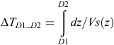and Vs(z) represents the S-wave speed at depth z. It follows from the definition of ΔT_{D1_D2} that

so

Solving the above equation for AVS_{10_20} gives

A similar procedure gives

The interval-averaged S-wave velocities for depth ranges of 10–20 m and 20–30 m (AVS_{10_20}, AVS_{20_30}) can be obtained from Equations 4 and 5 if the microtremor array method helps identify Rayleigh-wave phase velocities corresponding to wavelengths of 13, 25 and 40 m (C₁₃, C₂₅, C₄₀) and if they are used as substitutes for the average S-wave velocities for the topmost 10-, 20- and 30-m depth intervals beneath the surface (AVS_{0_10}, AVS_{0_20}, AVS_{0_30}) (e.g. Konno and Kataoka, 2000; Cho et al., 2008).

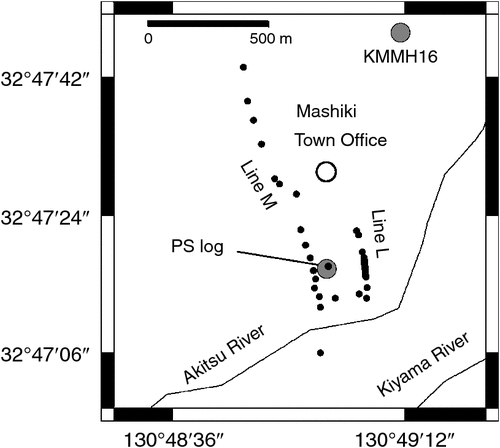
We conducted array measurements of microtremors at 18 sites along the 1.2-km-long survey line M in Mashiki (Figure 1) during 7–9 June 2016. A regular four-sensor array with a radius of 0.6 m, consisting of three sensors spaced evenly around a circle and another at the centre (Cho et al., 2013), and an irregular array of three unevenly spaced sensors (Cho et al., 2004) with side lengths of 5–7 m, were deployed at each site for 15-min recordings at a sampling frequency of 100 Hz.

Fig. 1.  A map of microtremor array measurement sites (black dots). The open circle shows the seat of the Mashiki town government. One of the grey circles indicates the site of an available PS log along survey line M, whereas the other shows the site of another PS log available at KiK-net Mashiki seismic station (KMMH16).

We also carried out observations along survey line L on 1 February 2017. We took 30-min recordings with a linear array of six seismic sensors spaced at 4-m intervals, and we conducted four sessions of the procedure to cover the total survey line length of 88 m. Further, we also took array recordings of the same type we had conducted along survey line M at three sites along an extension of survey line L. Hakusan Corporation’s JU215/JU410 servo accelerometer, which integrates a sensor with a data logger and is time-calibrated with a Global Positioning System, was used in all measurements.

The centreless circular array method of Cho et al. (2004, 2008, 2013) was applied to records of the regular four-sensor arrays and of the irregular three-sensor arrays, to obtain dispersion curves of Rayleigh-wave phase velocities. We also considered a set of three consecutive sensors in a linear array to be a ‘centred circular’ array of three sensors with a radius of 4 m and applied the spatial autocorrelation method of Aki (1957) to their records. The spectral analysis method, the procedure for estimating Rayleigh-wave phase velocities and the analysis parameters were the same as described in Cho et al. (2004), except that the fast Fourier transform segment length was set at 5.12 s. The method described here was applied to the Rayleigh-wave phase velocities evaluated at the individual sites to obtain estimates for interval-averaged S-wave velocities.

Figure 2 shows the Rayleigh-wave phase velocities estimated with the microtremor array method at the site of an available PS log (Yoshimi et al., 2016) (Figure 1). The figure also shows interval-averaged S-wave velocities calculated from the readings of C₁₃, C₂₅ and C₄₀. The relative residual errors of the interval-averaged S-wave velocities from those obtained directly from the PS log amounted to 2%, –14% and 20% for the AVS_{0_10}, AVS_{10_20} and AVS_{20_30}, respectively. For the sake of reference, we also conducted microtremor measurements at the site of another available PS log at KiK-net Mashiki seismic station (KMMH16) (Figure 1) and carried out similar comparisons. A circular array with a 26-m radius was also deployed there. The relative residual errors at that site were –30%, 3% and –19% for the AVS_{0_10}, AVS_{10_20} and AVS_{20_30}, respectively.

Fig. 2.  (a) A Rayleigh-wave phase velocity dispersion curve estimated by the microtremor method with a seismic-array radius of 0.6 m at the site of the PS log on line M. Also plotted on the panel are straight lines corresponding to wavelengths of 13 m, 25 m and 40 m. The phase velocity readings of the points of intersection between those straight lines and the dispersion curve represent C₁₃, C₂₅ and C₄₀, respectively. (b) The S-wave velocity structure beneath the PS log site. The interval-averaged S-wave velocities (IASVs) from the microtremor method and the PS log are indicated in red lines and black dashed lines, respectively. The original PS log is also shown in a black solid curve for reference.

Konno and Kataoka (2000) said that the AVS_{0_30} estimate from C₄₀ only represents a first approximation, partly because the C₄₀–AVS_{0_30} correlation is based only on numerical simulations and partly because the Rayleigh-wave phase velocity estimates from real microtremor array data contain measurement errors. The same can be said of C₁₃ and C₂₅, so the interval-averaged S-wave speeds that are derived from them should also be understood to be first approximations. In fact, they differed by up to 30% from the values based on PS logs.

The method presented here thus has its own limitations of accuracy, but it is recognisably effective in visualising relative spatial variations in S-wave speeds. For example, Figure 3 compares an S-wave velocity section, drawn by using the interval-averaged S-wave speed estimates from the microtremor data along survey line L, with available output of a surface-wave method at the same location (MLIT, 2017). It should be noted that the microtremor section shown here was drawn by spatial interpolation of the AVS_{0_10}, AVS_{10_20} and AVS_{20_30} values, which were taken to be representative S-wave velocities at depths of 5, 15 and 25 m, respectively. In other words, everything except at the X symbols is an interpolated value. It should also be noted that the two section drawings have different velocity scale bars.

Fig. 3.  Comparison of S-wave velocity sections along survey line L from a surface-wave study (MLIT, 2017) (top) and the microtremor method presented here (bottom). Note the two sections have different velocity scale bars. An earthquake fault cropped out on the surface at the location of the arrow during the Kumamoto earthquake. The X symbols in the microtremor section indicate the points of available data. The white curves represent velocity contours at 100 m/s intervals. The inverse triangles show the sites of microtremor array measurements.

The surface-wave method indicated low velocities in the neighbourhood of the arrow in the figure. An earthquake fault cropped out on the surface at the location of the arrow during the Kumamoto earthquake (Shirahama et al., 2016), which invites the question whether the low-velocity zone continues to greater depths. Low velocities were also indicated by the microtremor method at the same location. In addition, the microtremor section shows that velocities remain relatively low at least to a depth of 30 m beneath the earthquake fault outcrop, whereas the surface-wave method only visualised structures down to a depth of 15 m.

Figure 4 shows a microtremor section along survey line M. The line passes through an area of serious damage from the Kumamoto earthquake, with building collapse rates of 75% or more (MLIT, 2017), near an along-line distance of 1.0 km. A surface-wave study has also been conducted in the neighbourhood of that area (MLIT, 2017). Comparison found that the microtremor method produced an output pattern that was similar to the results of the surface-wave method in that area as well.

Fig. 4.  An S-wave velocity section along survey line M. The inverted triangles, representing the microtremor measurement sites, are colour-coded by measurement date: black for Day 1, light blue for Day 2 and green for Day 3. A velocity section from a surface-wave study (MLIT, 2017) is also shown by the side of the area covered by the study (black broken boundary). The grey circle indicates the site of an available PS log.

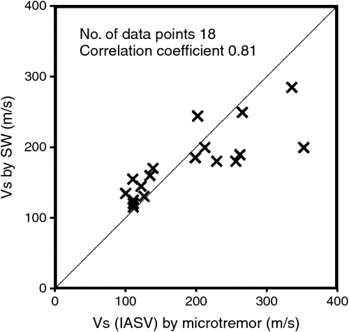
Certain differences, indeed, were recognised in the absolute velocity values. That led us to compare interval-averaged S-wave velocity estimates at representative points in the microtremor sections with corresponding S-wave velocity estimates in the surface-wave sections (Figure 5), although the two sets of quantities are primarily unsuited for direct comparison. That produced a correlation coefficient of 0.81, and the ratio between S-wave velocity estimates from the microtremor method and from the surface-wave method was found to be 1.04 ± 0.28 (standard deviation). The results indicated that there is meaningful correlation, despite the large variations.

Fig. 5.  Comparison of IASV estimates from the microtremor method (horizontal axis) with corresponding S-wave velocity estimates from surface-wave (SW) methods (vertical axis).

It should of course be noted that, as is evident from the figure, deviations grow with increasing depth. Quantitatively speaking, the estimates from the microtremor method turned out to be ~15% smaller on average than the estimates from the surface-wave method at a depth of 5 m and 23% larger at a depth of 15 m. The data from the deepest parts correspond to the lower boundary of the area covered by the surface-wave method, which is surrounded by a broken line in Figure 4. We believe there is a need to take account of both the question of the reliability of surface-wave methods (reliability of inverse analysis) and the question of the accuracy of the microtremor method presented here.

Small-scale seismic arrays excel in the flexibility of measurements. In the case of the present study, the introduction of miniature and irregular seismic arrays allowed efficient measurements, although very little space was available for deploying microtremor arrays because of seismic damage. That said, conducting dense and haphazard measurements would still be inefficient, no matter how efficient the measurement method may be in its own right, unless the method allows the velocity structure to be estimated on-site, so that decisions can be made on the next measurement location on the priority list. This is where our present method comes in handy. Our method allows the velocity structure to be visualised on the spot without putting a load on the computer, requiring only a system for estimating Rayleigh-wave phase velocities to be available at the measurement site. The analysis results do not depend on the analyser, because there is no leeway for the intervention of inversion parameters that might be selected arbitrarily by the analyser. Everybody can replicate the same results, so re-examination is easy even if a problem arises later. Our present method, therefore, has characteristics that make it suitable for use in preliminary on-site analysis.

In fact, we initially conducted measurements at 12 locations in a matter of only 6 h, including transit time, in order to get a rough picture of the pattern shown in Figure 4. We processed the data on the night of Day 1, whereupon we made decisions on the areas where we thought we needed denser records, and we carried out additional measurements at four sites on Day 2 and two sites on Day 3. As a result, Figure 4 captures a relatively good picture of the characteristics of steep changes in the velocity structure near along-line distances of 0.7 and 1.0 km. This illustrates the utility of our present method as a preliminary analysis tool for making the most of the flexibility of microtremor measurements using small-scale seismic arrays.

In the field of surface-wave methods, a simple conversion of the Rayleigh-wave phase velocity dispersion curve, more commonly known as the ‘one-third of the wavelength’ law (Gazetas, 1982; Standardization Committee of the Society of Exploration Geophysicists of Japan (SEGJ), 2008), has often been used as a classical tool for preliminary analysis. This technique consists of multiplying a wavelength value and a phase velocity value by respective scaling factors and assuming that the products represent the depth and the S-wave velocity, respectively. Empirically, that method indeed produces natural results, but its resolution fails significantly at depth. This is an inevitable problem, given that Rayleigh-wave phase velocities in long-wavelength (low-frequency) ranges correspond to subsurface properties integrated all the way from the surface to depth (Aki and Richards, 2002). Our present method has improved the resolution at depth by splitting the information contained in the Rayleigh-wave phase velocities into fragments of information by 10-m depth intervals. In that sense, our method could be recognised as an extension to the above-described simple conversion method.

Our method associates Rayleigh-wave phase velocities with subsurface structure models only through an empirical law. There is, therefore, no guarantee that theoretical Rayleigh-wave phase velocities, calculated from a subsurface structure model obtained with our method, will replicate the observed phase velocities. This represents a fundamental difference from more typical inversion methods, such as genetic algorithms and linearised inversion. But it is not hard to imagine that a theoretical Rayleigh-wave phase velocity dispersion curve based on a subsurface structure model obtained from our present method will explain observations to a certain extent, given that empiricism and theory have been so built to avoid too much deviation.

Figure 6, for example, compares a Rayleigh-wave phase velocity dispersion curve, calculated theoretically (Hisada, 1994, 1995) by using the interval-averaged S-wave velocity estimates, with a corresponding observed dispersion curve (site KMMH16). In the figure, the theoretical values represent fundamental-mode Rayleigh-wave phase velocities calculated by assuming a horizontally layered structure consisting of a semi-infinite medium underlying two 10-m-thick layers. The figure shows that theory agrees relatively well with the observations in a frequency range (5–10 Hz) corresponding to wavelengths from 13 to 40 m.

Fig. 6.  (a) Observed Rayleigh-wave phase velocities (solid curve) and (b) interval-averaged S-wave velocity estimates at site KMMH16. The left panel also shows, with open circles, the fundamental-mode Rayleigh-wave phase velocities calculated theoretically from a subsurface structure model based on the IASV estimates.

The above discussions, of course, are only intended to show the soundness of our present method and do not mean to say that more typical inversion methods are unnecessary. In fact, we do need, in various situations, approaches that are based on physical (theoretical) models. For example, our present method cannot even deal with the simple request that layering of the subsurface structure should be modelled after drilling data from the neighbourhood. An empirical law, before everything else, has limitations of accuracy.

At site KMMH16, array measurements of microtremors were taken and Rayleigh-wave phase velocity dispersion curves were shown by Arai and Kashiwa (2017) and Chimoto et al. (2016) as well. We have read their dispersion curves, applied our present method to each of them and compared the results with the interval-averaged S-wave speeds obtained in this study (Figure 6b). The differences in the interval-averaged S-wave speed estimates were found to grow with increasing depth. More specifically, the AVS_{0_10}, AVS_{10_20} and AVS_{20_30} were found to have standard deviations of 7%, 17% and 30%, respectively. Those variations are comparable in magnitude to the deviations from available PS logs as shown in the section ‘Application’ and likely indicate the limitations of our present method in terms of accuracy.

However, the so-called inverse analysis methods also require careful work. For example, the distribution of layers of a subsurface structure strongly influences the analysis results, and therefore, requires time for validation; an interested reader can compare between the inversion results in the publications of Arai and Kashiwa (2017) and Chimoto et al. (2016). Our present method has a different application. It is inferior to more typical inversion methods in terms of flexibility and accuracy, but we still believe it can be used effectively as a preliminary analysis tool for obtaining a rough picture of spatial variations in shallow structures by juxtaposing measurement and analysis results from a large number of sites.

We have presented a simple method for estimating interval-averaged S-wave velocities for depth ranges of 0–10, 10–20 and 20–30 m by using a Rayleigh-wave phase velocity dispersion curve obtained from array measurements of vertical-motion microtremors. This method could be understood as an extension, with enhanced resolution, on a conventional technique that consists of a simple conversion of a Rayleigh-wave phase velocity dispersion curve into an S-wave velocity profile. Our method is based on an empirical law that associates average S-wave velocities of subsurface structures with their Rayleigh-wave phase velocities. It uses only part of the information contained in Rayleigh-wave phase velocity dispersion curves and no other information on subsurface structures. It should be remembered, therefore, that the method only has limited precision, or in other words, may be subject to errors of up to a few tens of percent.

It has been shown, however, that our method produces output images that are similar to the results of surface-wave techniques insofar as the objective is to get an approximate picture of spatial variations in shallow structures by juxtaposing measurement and analysis results from a large number of sites. The output does not depend on the analyser, and it takes only simple algebra to obtain results once a Rayleigh-wave phase velocity dispersion curve has been estimated, so our method could be used effectively as a tool of preliminary analysis, particularly from the viewpoint of making the most of the flexibility of small-scale seismic arrays.

The authors declare no conflicts of interest.

References

Aki, K., 1957, Space and time spectra of stationary stochastic waves, with special reference to microtremors: Bulletin of the Earthquake Research Institute, University of Tokyo, 35, 415–457Aki, K., and Richards, P. D., 2002, Quantitative seismology (2nd edition): University Science Books.
Arai, H., and Kashiwa, H., 2017, Geotechnical boring and microtremor array surveys at KiK-net Mashiki Station: Summaries of technical papers of annual meeting Architectural Institute of Japan (in Japanese).
Chimoto, K., Yamanaka, H., Tsuno, S., Miyake, H., and Yamada, N., 2016, Estimation of shallow S-wave velocity structure using microtremor array exploration at temporary strong motion observation stations for aftershocks of the 2016 Kumamoto earthquake: Earth, Planets, and Space, 68, 206