

Australian carbon tetrachloride emissions in a global context
Paul J. Fraser A I , Bronwyn L. Dunse A , Alistair J. Manning B , Sean Walsh C , R. Hsiang J. Wang D , Paul B. Krummel A , L. Paul Steele A , Laurie W. Porter E J , Colin Allison A , Simon O’Doherty F , Peter G. Simmonds F , Jens Mühle G , Ray F. Weiss G and Ronald G. Prinn HA Centre for Australian Weather & Climate Research, CSIRO Marine & Atmospheric Research, 107-121 Station Street, Aspendale, Vic. 3195, Australia.
B UK Met Office, Fitzroy Road, Exeter EX1 3PB, UK.
C Monitoring & Assessment, EPA Victoria, Ernest Jones Drive, Macleod, Vic. 3085, Australia.
D School of Earth & Atmospheric Sciences, Georgia Institute of Technology, 311 Ferst Drive, Atlanta, GA 30332-0340, USA.
E Centre for Australian Weather & Climate Research, Bureau of Meteorology, 700 Collins Street, Docklands, Vic. 3008, Australia.
F Atmospheric Chemistry Research Group, School of Chemistry, University of Bristol, Cantock’s Close, Bristol, BS8 1TS, UK.
G Scripps Institution of Oceanography, University of California at San Diego, 8675 Discovery Way, La Jolla, CA 92093-0244, USA.
H Center for Global Change Science, Massachusetts Institute of Technology, 77 Massachusetts Avenue, Cambridge, MA 02139-4307, USA.
I Corresponding author. Email: paul.fraser@csiro.au
J Deceased.
Environmental Chemistry 11(1) 77-88 https://doi.org/10.1071/EN13171
Submitted: 6 September 2013 Accepted: 12 November 2013 Published: 19 February 2014
Environmental context. Carbon tetrachloride in the background atmosphere is a significant environmental concern, responsible for ~10 % of observed stratospheric ozone depletion. Atmospheric concentrations of CCl4 are higher than expected from currently identified emission sources: largely residual emissions from production, transport and use. Additional sources are required to balance the expected atmospheric destruction of CCl4 and may contribute to a slower-than-expected recovery of the Antarctic ozone ‘hole’.
Abstract. Global (1978–2012) and Australian (1996–2011) carbon tetrachloride emissions are estimated from atmospheric observations of CCl4 using data from the Advanced Global Atmospheric Gases Experiment (AGAGE) global network, in particular from Cape Grim, Tasmania. Global and Australian emissions are in decline in response to Montreal Protocol restrictions on CCl4 production and consumption for dispersive uses in the developed and developing world. However, atmospheric data-derived emissions are significantly larger than ‘bottom-up’ estimates from direct and indirect CCl4 production, CCl4 transportation and use. Australian CCl4 emissions are not a result of these sources, and the identification of the origin of Australian emissions may provide a clue to the origin of some of these ‘missing’ global sources.
Additional keywords: atmospheric and ‘bottom-up’ emissions estimates, Australian carbon tetrachloride emissions, emission estimates by inverse calculations and interspecies correlation, global carbon tetrachloride emissions.
Introduction
Carbon tetrachloride is an important ozone depleting substance (ODS), currently contributing ~10 % to both long-lived tropospheric chlorine and equivalent effective stratospheric chlorine (EESC), the latter being the major driver of stratospheric ozone depletion,[1,2] most obvious in the so-called Antarctic ozone ‘hole’.[3] Carbon tetrachloride was used over the past century as a degreasing and general solvent, fire retardant, refrigerant, grain fumigant, and, commencing over 70 years ago, CCl4 has been used as a feedstock chemical for the production of chlorofluorocarbons (CFCs), perchloroethylene (CCl2CCl2) and recently some hydrofluorocarbons (HFCs). Carbon tetrachloride is an over-chlorination by-product during the production of chloromethane, dichloromethane, vinyl chloride monomer (VCM, CH2CHCl) and most significantly trichloromethane (chloroform, CHCl3), itself a feedstock for HCFC-22 (CHClF2) production. Most by-product CCl4 is captured at the chemical production plant and recycled or destroyed before possible emission to the atmosphere.[1,4]
Concentrations of CCl4 have been measured almost continuously in the atmospheric marine boundary layer at mid-latitudes in the southern hemisphere since 1976 at Cape Grim, Tasmania,[5–9] periodically from 2005 to 2011 in the urban atmosphere at CSIRO Aspendale, Victoria and in air extracted from Antarctic firn, the oldest samples analysed to date being from the 1930s.[10] Global abundances of CCl4 have been measured as part of the Advanced Global Atmospheric Gas Experiment (and its precursor programs: Atmospheric Lifetime Experiment – ALE, Global Atmospheric Gases Experiment – GAGE) since 1978[1,6–8,11] and in the NOAA (National Atmospheric and Oceanic Administration, USA) global in situ measurement program since 1992.[1,12] Carbon tetrachloride abundances in the atmosphere peaked in the early 1990s and are now declining slowly,[1,6,8,11,12] in response to Montreal Protocol production and consumption controls (100 % phase-out) adopted by the developed world in 1996 and the developing world in 2010.
The observed decline in atmospheric CCl4 is less rapid than expected under the Montreal Protocol, presumably because of a longer than estimated atmospheric lifetime, or underestimated or unidentified emissions, with larger emissions the most likely cause.[1] Elimination of future CCl4 emissions, which, as a first step, requires the identification of all globally significant CCl4 sources, is now projected to have a larger effect on EESC than thought previously.[13] For example, total elimination of CCl4 emissions after 2010 will reduce future mid-latitude EESC over the period 2010–2045 by ~8 % and hasten ozone recovery at mid-latitudes by 5 years (from 2050 to 2045).[13]
Carbon tetrachloride data from Cape Grim and other strategic sites around the globe have been used to derive global[1,6,8,12] and regional CCl4 emissions (Asia,[6,14–16] ~75 % of global emissions[6]; Africa,[6] ~10 %; North and South America,[6,17,18] ~10 %; Europe,[6] ~5 %; Australia and New Zealand,[6,19] <1 %), using inverse modelling and inter-species correlation (ISC) techniques, the latter employing carbon monoxide, or HCFC-22, or fossil-fuel carbon dioxide as the marker or reference species. Global CCl4 emissions derived from atmospheric data by inverse modelling were ~60 Gg year–1 in 2008,A declining slowly by 3 % year–1.[1,6]
Australian CCl4 emissions have been estimated by ISC from Cape Grim data, with carbon monoxide as the reference species, at 150 ± 45 Mg in 1996,[19] ~0.5 % of global emissions. These Australian emissions are lower, although uncertainties overlap, than CCl4 emissions (320 ± 160 Mg, 1996–2004[6]) estimated for Australia (assuming Australian emissions are 80 % of emissions from Australia plus New Zealand) from AGAGE data by inverse methods using MATCH (Model for Atmospheric Chemistry and Transport), a 3-D Eulerian transport model, (2.8 × 2.8°, 28 levels) and a Kalman filter.[6,20] They are significantly lower than a preliminary version of the AGAGE–MATCH inversion for Australia (2500 ± 1000 Mg) published by United Nations Environment Programme (UNEP) in 2009.[4] This latter inversion was initiated with an unrealistically large prior estimate of Australian CCl4 emissions based on an economic activity (gross domestic product)-based fraction of global emissions.
In this paper we update estimates of global and Australian CCl4 emissions from global and Cape Grim AGAGE data, using inverse modelling, by the AGAGE 2-D 12-box model,[21] the InTEM (Inversion Technique for Emission Modelling)–NAME (Numerical Atmospheric dispersion Modelling Environment)[22] and a revised version of the ISC methodology. Air mass trajectory data are used to identify local Australian CCl4 source regions, and possible sources, that are influencing the Cape Grim and Aspendale data. The Australian emission data may suggest sources of CCl4 emissions that are not currently included in global ‘bottom-up’ estimates and that may be globally significant.
Experimental
Several instruments have been used to measure CCl4 in situ at Cape Grim since 1976, intermittently in situ at CSIRO Aspendale since 2005 and in Antarctic firn air. Instrumental, operational and calibration protocols for the CSIRO, ALE, GAGE and AGAGE CCl4 measurement programs at Cape Grim and at Aspendale have been published (Table 1). The Cape Grim (and other sites) ALE, GAGE and AGAGE in situ data are available from the publically accessible AGAGE data archive (see http://agage.eas.gatech.edu/data.htm, accessed October 2013).

|
All other CCl4 data used in this paper are available from CSIRO on request (paul.fraser@csiro.au). The ALE, GAGE, AGAGE and CSIRO data are reported in the SIO05 gravimetric scale; the CSIRO data were placed on an approximate SIO05 scale using the average ratio of ALE to CSIRO monthly means during the ALE–CSIRO overlap period (1978–1982). The firn data were originally reported in the SIO98 scale,[10] but are now reported in the SIO05 scale; the scales are identical for CCl4.
Throughout the ALE–GAGE–AGAGE program various approaches have been used to identify background or baseline data and pollution episodes (enhancements above baseline from regional sources). These have involved, at various times, meteorological data, air mass trajectories and correlations between pollution marker species. An automated, statistically based approach to identifying baseline data and pollution episodes, utilising 2.5 standard deviations from polynomial best-fits, has been developed as the AGAGE database and has grown to currently over 50 trace gas species.[11,23]
Results and discussion
Australian and Antarctic CCl4 observations
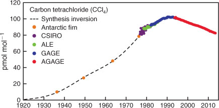
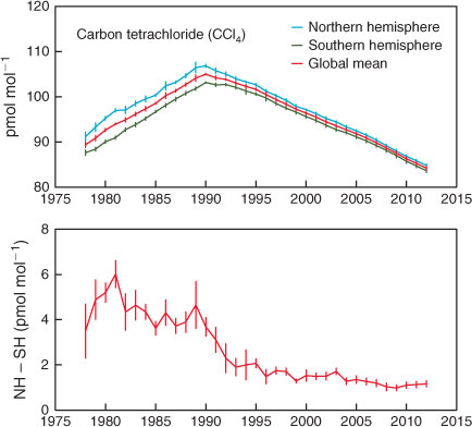
The Cape Grim in situ and Antarctic CCl4 data (background monthly means) are shown in Fig. 1.
|
Based on Antarctic firn air data, and assuming CCl4 is conservative in firn air over the storage period, CCl4 levels in the Southern Hemisphere in the early 20th century were less than 10 ppt (parts-per-trillion, dry air mole fraction × 1012), growing steadily in the atmosphere, reaching ~80 ppt by the mid-1970s when quasi-continuous measurements commenced at Cape Grim. Carbon tetrachloride abundances in the atmosphere peaked in the Southern Hemisphere atmosphere at 102 ppt in 1990 and are now declining slowly (1.0 ppt year–1, currently 1.2 % year–1).[1,6,8,12] The Antarctic firn data are consistent with no significant pre-industrial atmospheric levels of CCl4; however, given the uncertainties in the inversion of the Antarctic firn data, a pre-industrial level of ~5 ppt cannot be ruled out.[10,24]
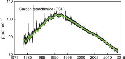
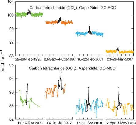
The complete CCl4 data record collected at Cape Grim is shown in Fig. 2. Evidence of the influence of local or regional sources of CCl4 is seen in the regular deviations above baseline, so-called ‘pollution episodes’. The Cape Grim pollution episodes (Fig. 3, gas chromatography–electron capture detection (GC-ECD), 1994–2012), used quantitatively to estimate regional emissions, show typical maximum concentrations less than 2 ppt above baseline, and are less intense than those seen at Aspendale (typical maximum less than 6 ppt above baseline), suggesting Aspendale is closer to the regional CCl4 sources (see below) than Cape Grim. The Aspendale gas chromatography with mass spectrometric detection (GC-MSD) CCl4 data are not suitable for long-term trends because of possible calibration discontinuities and unresolved analytical problems, and are therefore not used quantitatively to estimate emissions, but are used qualitatively to identify possible CCl4 source regions and locations.
|
|
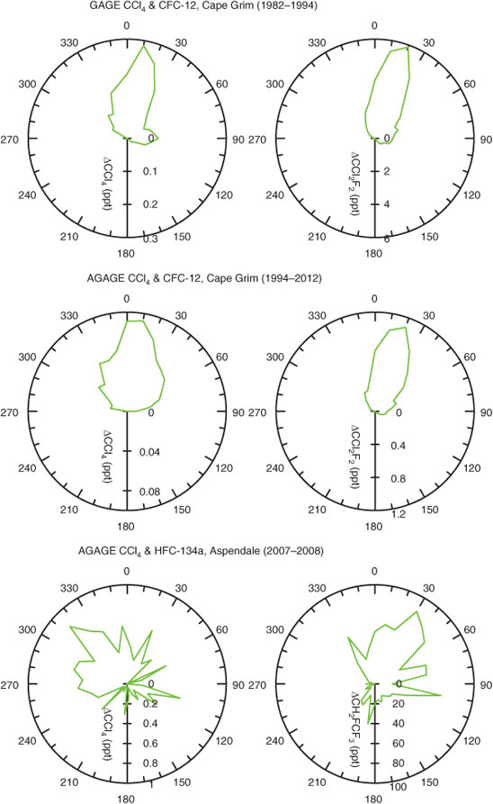
To date the ALE (1978–1985) and GAGE (1981–1994) GC-ECD data at Cape Grim have not been analysed using ISC or InTEM–NAME to derive Australian CCl4 emissions. On average the GAGE data show significantly higher (factor of 2–3) pollution episodes than the AGAGE data (Figs 3, 4), presumably reflecting higher emissions during the GAGE period compared to the AGAGE period. The ratio of the average magnitudes of GAGE–AGAGE CCl4 pollution ‘roses’ (Fig. 4) can be used to derive average Australian CCl4 emissions during the GAGE period (early-1980s to mid-1990s; see below).
|
The CCl4 and CCl2F2 (CFC-12) pollution ‘roses’ (trace gas deviations above baseline as a function of wind direction) seen at Cape Grim during GAGE (1981–1994) and AGAGE (1994–2012) periods are shown in Fig. 4, together with the CCl4 and HFC-134a (CH2FCF3) pollution ‘roses’ for Aspendale. At Cape Grim, the CCl4 and CFC-12 polluted air masses arrive at Cape Grim in the northerly sector (30°W – 30°E). Air mass trajectories clearly show that the origin of this pollution is the Melbourne–Port Phillip region. The clear decline in Port Phillip emissions for CCl4 (and CFC-12) can be seen at Cape Grim from the GAGE (1981–1994) to AGAGE (1994–2012) periods: a factor of 2.5 decline in CCl4 emissions and a factor of 5 decline in CFC-12 emissions. Interestingly the GAGE Cape Grim CCl4 pollution data show an easterly ‘lobe’ that largely disappears in the AGAGE data, suggesting a variable northern coastal Tasmanian CCl4 source (discussed below).
At Aspendale, there is a clear difference in the wind direction-dependence of CCl4 and HFC-134a pollution episodes, with maximum concentrations of HFC-134a in the north-east sector and for CCl4 in the north-west sector. The HFC-134a pattern is consistent with emissions proportional to population density (domestic and commercial refrigeration, automobile air conditioning), whereas the CCl4 pattern is consistent with emissions focussed on the heavy industry region west of central Melbourne.
Global CCl4 observations and emissions
AGAGE global, Northern Hemispheric (NH) and Southern Hemispheric (SH) CCl4 data are shown in Fig. 5. Global concentrations peaked at 104 ppt in 1990 and since 1995 have been declining linearly at 1 ppt year–1 (currently 1.1 % year–1).[6,8,11] By 2011, global CCl4 concentrations had declined to 84 ppt. There are periods of significant and sustained difference (NH–SH) in CCl4 concentrations: 1.6 ± 0.2 ppt, 1995–2003; 1.2 ± 0.1 ppt, 2004–2012). This suggests that the predominantly NH emissions that sustain this inter-hemispheric difference were approximately constant during these periods. The inter-hemispheric difference for CCl4 in the absence of emissions is expected to be small because the surface CCl4 sinks (oceans, soils) are small (<5 % of total emissions) and offsetting (soils predominantly NH, oceans predominantly SH) and the stratospheric sink is similar in both hemispheres.[1] Reductions in NH–SH differences occurred after 1989, 1995 and 2003, which approximately reflect the timing of significant Montreal Protocol control measures for CCl4 (1989: Montreal Protocol baseline reference consumption year for developed countries; 1995–1996: 85 and 100 % phase-out for developed countries; 2005: 85 % phase-out of developing world consumption compared to 1998–2000 average; 2010: 100 % phase-out for developing countries).
|
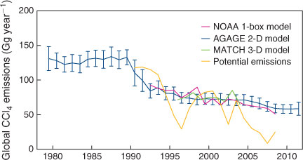
Global emissions derived from AGAGE and NOAA global CCl4 data, by the NOAA 1-box model,[1] the AGAGE 12-box 2-D model[21] and the 3-D MATCH model–Kalman filter[6,20] are shown in Fig. 6. Global CCl4 emissions derived from atmospheric data by inverse modelling, assuming a 26-year atmospheric lifetime for CCl4, are currently declining slowly (by 3 % year–1 since the early 1990s), from an approximately constant 130–140 Gg throughout the 1980s to 59 ± 6 Gg by 2008,[1,6] remaining steady at 59 ± 9 Gg by 2011. The 5-year (2007–2011) average global CCl4 emissions were 59 ± 7 Gg and the previous 5-year (2002–2006) average emissions were 70 ± 7 Gg.
|
Also shown in Fig. 6 are ‘bottom-up’ or ‘potential’ global emissions of CCl4, the latter based on national CCl4 production and consumption data reported to UNEP under Article 7 of the Montreal Protocol, less data on CCl4 used as a feedstock, with concomitant 2 % fugitive emissions and CCl4 recycled or destroyed, a process assumed to be 75 % efficient.[1,4] These ‘bottom-up’ emission estimates are highly variable, reflecting significant year-to-year variations in reported consumption data from individual nations. In deriving these ‘potential’ emissions, attempts were made to ‘fill-in’ missing consumption data,[1] but it is clear that the quality of the reported UNEP production and consumption data could be improved.
Australian CCl4 emissions
Carbon tetrachloride emissions from the Melbourne–Port Phillip region (28 ± 8 Mg in 1996) have been estimated utilising in situ GC-ECD measurements from Cape Grim, Tasmania, employing an ISC technique with co-incident CO measurements as the marker species.[19,25,26] These original CCl4 emission estimates were based on CO emissions from the Melbourne–Port Phillip region (670 Gg in 1996), which have been estimated at 700–800 Gg during the 1970s and 1980s,[27] declining to 600–700 Gg during the 1990s and remaining at ~600 Gg throughout the 2000s[27,28] (see http://www.npi.gov.au/npi-data/, accessed July 2013). Corresponding Australian CCl4 emissions of 150 ± 45 Mg in 1996 were derived by scaling the Melbourne–Port Phillip emissions on a population basis.[29]
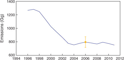
There has been a recent revision of the CO emissions estimate for the Melbourne–Port Phillip region (Fig. 7). The 2006 emissions are now estimated to have been ~800 Gg, with the increase in the emissions estimates attributable to redefining the aerial extent of the Port Phillip region and the effect of ambient temperature on emissions, which results in increased estimates of CO emissions from vehicles and reduced emissions from wood heaters.[30]
|
The Victorian Environmental Protection Agency (EPA) has measured CO concentrations at several sites throughout the Port Phillip air-shed since 1996.[30,31] Assuming that the average CO levels observed in the Port Phillip air-shed are proportional to the average CO emissions in the air-shed, long-term trends in CO emissions can be inferred and can be scaled by the revised Port Phillip CO emission estimate for 2006 (796 ± 80 Gg).[30]
Port Phillip CO emissions declined rapidly from over 1200 Gg in the mid-1990s to 800 Gg in the early 2000s and have remained approximately constant at 700–800 Gg from 2003 to 2011, despite increasing vehicle numbers, the primary source of Port Phillip CO emissions.
Melbourne–Port Phillip CCl4 emissions have been recalculated, for 1995–2011, using ISC with these revised CO emissions and Cape Grim GC-ECD CCl4 observations. NOAA air mass back trajectory analyses[32] and correlations with urban marker species (CFC-12, CCl2F2; HFC-134a, CH2FCF3) are used to confirm that the CCl4 pollution events seen at Cape Grim (and used to derive CCl4 emissions) originate from the Melbourne–Port Phillip region. Air-mass back trajectories are used to exclude air parcels that have passed over the Latrobe Valley east of Melbourne–Port Phillip, which has a disproportionately large CO source, with respect to population, from coal-fired power stations.
The ISC emissions calculations can be skewed if the Melbourne–Port Phillip emissions include significant contributions of CO from biomass burning, in particular from bushfires (wildfires) in or close to the Port Phillip region. A satellite-based bushfire-monitoring tool (Sentinel Hotspots, Geoscience Australia, CSIRO and Defence Imagery and Geospatial Organisation, Australia, http://sentinel.ga.gov.au/, accessed July 2013), that provides information about fire dates, locations and areal extent across Australia, is used to identify CO pollution events at Cape Grim that are affected by biomass burning. Sentinel was not available before 2003, when an alternative method to identify biomass burning events was used based on marker species such as CH3Cl. Cape Grim CO pollution episodes that are affected by biomass burning are excluded from this analysis.
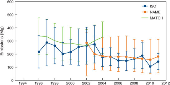
The Australian CCl4 emissions are derived from Port Phillip emissions, using a population-based scale factor of 4.8 ± 1.0. This population-based scale factor is derived from ABS (Australian Bureau of Statistics) population numbers for Australia and the Port Phillip region. These are known accurately, and their ratio (the scale factor) is largely time-invariant. However, there is uncertainty in the scale factor that arises because it is possible the Cape Grim pollution episodes selected for this study are influenced by additional emissions from outside the Port Phillip region, despite our best efforts to confine this study to those pollution episodes originating entirely from the Port Phillip region. This uncertainty can be estimated by calculating CO per capita emissions for Port Phillip and surrounding regions that could also influence Cape Grim data. These per capita emissions show a variability of ±20 % and this is the uncertainty assigned to the scaling factor and is incorporated into the uncertainties in the calculated CCl4 emissions by ISC. The annual mean Australian CCl4 emissions by the ISC methodology are derived from a consecutive 3 years of data (i.e. 2010 emissions are calculated from 2009–2011 data) for the period 1996–2011 (Fig. 8).
|
Australian CCl4 emissions have been estimated by inverse modelling using InTEM–NAME; NAME is a global 3-D Lagrangian particle dispersion model. InTEM–NAME has been used to estimate UK and European emissions of CFCs, HCFCs, HFCs, methane and nitrous oxide from AGAGE atmospheric observations at Mace Head, Ireland.[33–37]
Using Cape Grim CCl4 data, InTEM–NAME ‘sees’ emissions from Victoria, Tasmania and New South Wales. The Australian emissions are calculated from InTEM–NAME Victorian, Tasmanian and NSW emissions using a population-based scale factor of 1.7 and, as with ISC, each annual mean is derived using a consecutive 3 years of CCl4 data (Fig. 8).
Australian CCl4 emissions obtained from ISC have declined from ~270 Mg in the mid-to-late 1990s to ~145 Mg in the late 2000s, a decline of 40–50 % in a decade. The 1996–2004 ISC average emissions are 240 ± 35 Mg, 25 % lower than the MATCH estimates for Australia (320 ± 160 Mg) for the same period.[6] The InTEM estimates of Australian CCl4 emissions have declined from 250 ± 125 Mg in 2002–2003 to 170 ± 80 Mg in 2010–2011. Although the ISC emission estimates show significant year-to-year variability, over the period 2002–2011 mean ISC and InTEM emissions of CCl4 for Australia agree to within 7 % (ISC higher). Since 2004, ISC and InTEM–NAME CCl4 annual emissions for Australia have averaged 165 ± 45 Mg. Based on the intensity of pollution episodes at Cape Grim during the GAGE period (1981–1994), compared to the AGAGE period (1994–2012), Australian CCl4 emissions during 1981–1994 were likely to have been in excess of 400 Mg year–1.
Two independent inversions (InTEM, MATCH) and ISC show significant CCl4 emissions in the Australian region, declining from 250–350 Mg in the late 1990s to 120–180 Mg in the early 2010s. These emissions are unlikely to arise from the production (direct or indirect), transport and use of CCl4, because there has been no CCl4 production, no organo-chlorine chemical production using CCl4 as feedstock and no significant imports of CCl4 into Australia since the 1980s. In the following section, possible CCl4 source regions are identified that may provide clues as to the origin(s) of these Australian CCl4 emissions.
Potential CCl4 sources in the Port Phillip region
The Aspendale GC-MSD CCl4 data show clear pollution episodes, and four of the more significant are shown in Fig. 3. The air mass trajectories corresponding to these four episodes are shown in Fig. 9. All four trajectories (December 2006, July 2007, April and May 2010) arrived at Aspendale, having previously passed over central Melbourne or the industrial area immediately west (within 10 km) of central Melbourne. The source of the local CCl4 emissions may be central Melbourne or the industrial or chemical production areas west-south-west of central Melbourne.[38] This is also suggested from the Aspendale pollution ‘rose’ data shown in Fig. 4.
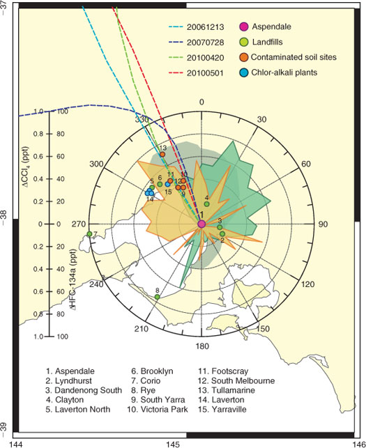
|
The Victorian EPA has identified four sites (Fig. 9: site #9 South Yarra – a council depot, #10 Victoria Park – a former dry cleaning plant, #11 Footscray and #12 South Melbourne), in or adjacent to central Melbourne, containing CCl4 contaminated soil, and a further site at Tullamarine (#13), a former landfill and toxic waste storage facility (M. Bannister, EPA Victoria, pers. comm., 2011). Vent pipe CCl4 concentrations at Tullamarine have been recorded in excess of 1 ppb. All five sites are in the north-west sector with respect to Aspendale. The Victoria Park site is a former textile mill and dry-cleaning plant that has been estimated to contain ~1500 Mg of CCl4 contaminated soil, which is in the process of being removed for treatment at the Corio landfill, which treats toxic waste (site #7).
Melbourne–Port Phillip has five active landfill and toxic waste processing sites (Fig. 9): Lyndhurst – site #2, which processes Melbourne’s highest level toxic waste, and Dandenong South – site 3 (both SE of Aspendale), Laverton North – site #5 and Brooklyn – site #6, which is Melbourne’s largest capacity toxic waste treatment facility (both north-west of Aspendale) and Corio (west of Aspendale), all capable of processing CCl4 contaminated soil. An additional site #4 (Clayton) may have received toxic waste (including CCl4 contaminated waste) before the current EPA toxic waste handling licensing arrangements (M. Bannister, pers. comm.). The Aspendale CCl4 data show significant enhancements above baseline in the north-west sector and possibly in the SE sector (Fig. 9).
Daytime (1400–1500 hours eastern standard time, EST) air samples upwind and downwind of the Lyndhurst toxic waste treatment facility (Fig. 9, site #2) were collected in stainless steel flasks in August 2011 and analysed for CCl4 at CSIRO Aspendale. Upwind sampling gave mean CCl4 concentrations of 77 ppt (range 71–84 ppt) from three samples and downwind sampling gave 81 ppt (range 73–88 ppt) from three samples. Although the measurement ranges overlap, the Lyndhurst facility would appear to be a source of CCl4 emissions.[29] This is consistent with Aspendale in situ CCl4 data, which shows small CCl4 enhancements in the south-east sector, which contains the Lyndhurst facility.
In addition, Melbourne has three active chlor-alkali plants (membrane technology) in and around Laverton – site #14 (north-west of Aspendale) producing a total of ~50 Gg year–1 of chlorine, hypochlorite, hydrochloric acid and chlorinated organics (chlorinated paraffins and herbicides), and one former plant (mercury – Hg – cell technology) at Yarraville – site #15 (Fig. 9). All of these sites are in the north-west sector with respect to Aspendale. UNEP has identified chlor-alkali plants as a possible source of inadvertent CCl4 production.[4]
CSIRO conducted a 3-year experiment (2006–2008) at the Rye landfill (site #8, Fig. 9), a modern, capped waste disposal facility that accepts largely domestic and commercial, but not industrial, waste. The Rye landfill generates electricity from the combustion of landfill gas.[39] Using flux chamber techniques, small fluxes of CCl4 were detected emanating from the active waste cells (1 µg m–2 h–1) and from the capped waste cells (0.2 µg m–2 h–1). The Rye landfill gas, which contained 0.2 ppb of CCl4, is used to fuel a modified, diesel-powered generator to produce electricity. There was no detectable CCl4 in the exhaust gas, indicating complete CCl4 destruction in the gas-powered diesel engine, which is not unexpected, given the combustion temperatures of ~1000 °C that operate in such an engine. The study concluded that this capped landfill, which handled domestic and commercial waste, was not a significant source of trace gas (including CCl4) emissions in the Port Phillip region. A similar conclusion was reached for CFC and 1,1,1-trichloroethane (methyl chloroform, CH3CCl3) emissions (insignificant emissions on a global scale) from a study of landfills in the USA and UK. Unfortunately CCl4 was not one of the trace gases studied.[40]
The Aspendale data show that there are likely CCl4 sources to the north-west and south-east of Aspendale, sectors that contain all of the Melbourne–Port Phillip chlor-alkali plants, CCl4 contaminated soil sites and toxic waste treatment plants.
The Cape Grim data suggest there are variable CCl4 source(s) in the easterly sector from Cape Grim (Fig. 4). This sector contained chorine-based paper pulp bleaching plants, employing Cl2/ClO2/OCl– based bleaching processes, associated chlor-alkali plants and toxic waste treatment facilities, at Burnie (120 km east of Cape Grim) and Wesley Vale (170 km east of Cape Grim) from the late 1930s to 2010. Both chlor-alkali plants and associated paper pulp bleaching activities ceased operations in 2010. During the GAGE period (1981–1994) both the Burnie and Wesley Vale chlor-alkali plants were largely Hg-cell technology and in the AGAGE period (1994–2012), the chlor-alkali plants used membrane technology exclusively (the technology transition occurred at both sites during 1988–1990). There is a clear reduction in CCl4 emissions from northern Tasmania from the GAGE to the AGAGE periods – perhaps the Hg-cell chlor-alkali technology was a source of CCl4 emissions.
UNEP has identified these facilities and activities as potential CCl4 sources.[4] Presumably the CCl4 emissions observed in the Port Phillip region, likely from toxic waste and possibly from chlor-alkali production facilities, are occurring in other Australian urban–industrial regions. Of particular interest is Sydney, which, in addition to several toxic waste treatment facilities and chlor-alkali plants, was historically the only Australian city that hosted CCl4, CFC and HCFC production facilities that were phased-out in the late-1980s–early 1990s. CSIRO is planning to install an in situ CCl4 monitoring facility (GC-MSD), similar to the Aspendale and Cape Grim facilities, in the Sydney region in 2014, data from which will likely significantly reduce the uncertainties in deriving Australian CCl4 emissions.
Other possible regional CCl4 sources
Chemical feedstock use
The three major chemical feedstock uses of CCl4 are in the production of HFCs (30 %), PCE (25 %) and CFCs (10 %). VCM production represents a minor (<10 %) feedstock use, as do several other minor uses, for example pyrethroid production.[41] Estimates of national uses of CCl4 as feedstock are not available from UNEP, although the data are collected, but considered commercial-in-confidence, from nations reporting their ODS production and consumption data.[41] UNEP do release the feedstock data as a global estimate.
CFCs and PCE are no longer manufactured in Australia, but VCM is likely still produced, although not involving CCl4 (see Vinyl Council of Australia, http://www.vinyl.org.au, accessed July 2013). It is possible that there is no Australian feedstock use and emissions of CCl4.
An upper limit of Australian CCl4 emissions from unidentified feedstock use (<5 Mg) can be obtained from global feedstock use data (~180 Gg in 2010), assuming these unidentified (in Australia) uses represent <5 % of the global feedstock use distribution of CCl4 (0.5–1.5 % of which may occur in Australia) and also assuming the upper limit of fugitive emissions from feedstock use (5 %).[41] Although very uncertain, chemical feedstock use of CCl4 may be a source of 0–5 Mg year–1 of Australian CCl4 emissions.
Biomass burning
Cape Grim is an atmospheric observing site that is occasionally affected by bushfire (wildfire) plumes from continental and Bass Strait island fires. The former are usually mixed with urban emissions from the Port Phillip region, given the nature of the meteorology that transports Australian continental air to Cape Grim, but the latter are ideal for uniquely identifying the effect of biomass burning on atmospheric trace gas and aerosol composition.[42]
Three late-summer Bass Strait bushfire plumes from Robbins Island (15–30 km west of Cape Grim: February 1995, February 2006, March 2008) have been examined in detail. The data show clear evidence of CH3Cl and CHCl3 enhancements in the local bushfire plumes but no evidence of any production of CH2Cl2 or CCl4.
Soil and wetland emissions
Coastal soils and salt marshes have been reported as either small sources or sinks for CCl4. From 75 flux chamber experiments on coastal soils and salt marshes in southern California (1997–2000), emissions of CHCl3 (0.05 ± 0.06 µg m–2 h–1) and CCl4 (0.005 ± 0.010 µg m–2 h–1) have been detected, with higher emissions of CCl4 from decaying kelp (0.09 µg m–2 h–1), corresponding to a global CCl4 source from kelp of 0.1 Gg year–1.[43] However, from 13 flux chamber experiments on coastal salt marshes in east China (2004–2005) during spring to autumn, sinks for CHCl3 (1–3 μg m–2 h–1) and CCl4 (0.1–0.3 μg m–2 h–1) have been found.[44]
The possible effects of coastal soils and salt marshes on CH3Cl, CH2Cl, CHCl3 and CCl4 data at Cape Grim have been investigated. From 18 flux chamber experiments throughout 2002 on salt-affected soils (improved pasture, eucalypt and melaleuca forest soils, native grassland, tidal flats) in the vicinity of Cape Grim, emissions of CHCl3 (1–3 µg m–2 h–1) were identified and a small sink for CH3Cl (0–1 µg m–2 h–1) was found, but no significant emissions (or uptake) of CH2Cl2.[45] The data from these experiments have been re-examined and, similar to CH3Cl, a small terrestrial CCl4 sink in the Cape Grim region was identified (0–1 µg m–2 h–1).
Typical air mass trajectories from the Melbourne–Port Phillip region to Cape Grim spend >95 % of the trajectory duration over the ocean and thus the effect of this small coastal soil CCl4 sink on Cape Grim CCl4 observations is likely negligible. Air masses on route from Melbourne–Port Phillip to Cape Grim spend on average less than 12 h over the ocean waters of Bass Strait. Given the oceanic sink CCl4 lifetime of 90–100 years,[1] this sink will have negligible effect on the CCl4 pollution episodes arriving at Cape Grim.
Water chlorination
Chlorination by Cl2 or OCl– is a widely used method to reduce the bacterial levels in waste and drinking water, leading to the in situ production of chlorinated organic species, in particular trihalomethanes.[46] Carbon tetrachloride has not previously been reported in the literature as a product of waste or potable water chlorination. However, significantly enhanced CCl4 concentrations (up to 30 ppb) have been observed in indoor-air environments associated with the domestic use of hypochlorite (OCl–) bleach products.[47] The possible global magnitude of such a CCl4 source has not been estimated, but this observation raises the question as to whether water chlorination by Cl2/OCl– could lead to CCl4 emissions to the atmosphere.
With this in mind, we have investigated possible emissions of CH3Cl, CH2Cl2, CHCl3 and CCl4 from a domestic chlorinated swimming pool on the southern perimeter of Melbourne.[29] A dynamic flux chamber[39,45] experiment was carried out on a 30 000-L pool during March (early autumn) 2012 (Fig. 10). The chamber was flushed with air of known CH3Cl, CH2Cl2, CHCl3 and CCl4 concentrations at a measured rate. The pool water temperature was steady at 20 °C. The residence time in the chamber was ~1 h. The ‘active’ chlorine (OCl–) levels in the pool were varied (2–8 ppm), which correlated with resultant trace gas emission rates. Significant emissions of CH3Cl (5–7 µg m–2 h–1), CHCl3 (600–1200 µg m–2 h–1) and CCl4 (0.2–0.3 µg m–2 h–1) were detected, but the emissions of CH2Cl2 (<0.1 µg m–2 h–1) were not significant.
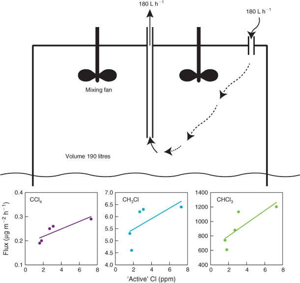
|
Assuming there are 1 million pools in Australia with an average surface area of 30 m2 and an ‘active’ Cl level of 1–2 ppm (as recommended by pool chemical suppliers, see Australian Bureau of Statistics, AUSSTATS, 2007, www.abs.gov.au/, accessed July 2013), the annual Australian emission of these species from swimming pools to the atmosphere could be ~150 Mg of CHCl3, 1–2 Mg of CH3Cl and 0–0.2 Mg of CCl4. Swimming pools are not a significant source of CCl4 in Australia. If we assume 50 % of Australia’s chlorine consumption is used to treat water (including swimming pools), and that the CCl4 flux from all water treatment as a function of ‘active’ chlorine levels is approximately the same as measured for swimming pools, then Australian CCl4 production from water treatment by chlorination could be up to 0.5 Mg year–1, only a small fraction of the current annual Australian emission (165 Mg).
This result is supported by the Aspendale CCl4 observations where the source pattern (Fig. 4, predominantly west of central Melbourne) is not consistent with the expected pattern from water chlorination, which would likely correlate with the population distribution, as does HFC-134a for example (Fig. 4).
Global implications
Presumably these currently unaccounted-for CCl4 emissions that are probably coming from contaminated soils and toxic waste treatment facilities, and possibly chlor-alkali plants, as seen in Australia, are occurring world-wide. Australian emission of ODSs and greenhouse gases (GHGs) are currently typically 0.5–1.5 % of global emissions (CO2: 1.3 %, CFCs: 0.9 %, HCFCs 0.6 % and HFCs 1.7 %).[29,48] Assuming the Australian CCl4 emissions (165 ± 45 Mg, 2004–2011) are 1 ± 0.5 % of these unaccounted-for global emissions, then the global emissions of CCl4 from these sources could be 10–30 Gg year–1. The ‘gap’ between ‘bottom-up’ and ‘top-down’ estimates for global CCl4 emissions since 2004 has averaged 40 ± 20 Gg. Thus these unaccounted-for CCl4 emissions could, on average, be responsible for approximately half (25–75 %) of this ‘gap’.
This assessment is, at best, barely qualitative. Cape Grim ‘sees’ global CCl4 emissions in the observed baseline data and regional CCl4 emissions from south-east Australia in the pollution episode data. Extrapolating these latter, regional emissions to emissions on a global scale is highly uncertain. However the results do suggest that additional, strategic regional studies (in particular in Europe, North America and Asia) on possible CCl4 emissions from contaminated soils, toxic waste treatment facilities and chlor-alkali plants may significantly reduce the ‘gap’ between ‘bottom-up’ and ‘top-down’ estimates of global CCl4 emissions.
Summary
In response to global restrictions on the production and consumption of CCl4, Southern Hemispheric and global atmospheric abundances of CCl4 continue to decline at 1.1–1.2 % per year since their peak in 1990. Based on atmospheric observations, global CCl4 emissions declined steadily (~3 % year–1) from ~140 Gg year–1 throughout the 1980s to ~60 Gg year–1 in the late 2000s. There has not been a significant decline in emissions (~60 Gg year–1) since 2008. This level of emissions is unlikely to be attributable to fugitive CCl4 releases from the production (direct and indirect), transport and use of CCl4.[1] Other CCl4 emission sources appear to be active.
Australian CCl4 emissions have been estimated from global CCl4 observations using a global inverse model (MATCH–Kalman filter) and from Cape Grim CCl4 observations using inverse (NAME–InTEM) and ISC methodologies. Australian emissions of CCl4 are also in decline, from 250–350 Mg in the late 1990s to 120–180 Mg in the early 2010s, averaging 165 ± 15 Mg (2004–2011). These emissions are unlikely to arise from the production (direct or indirect), transport and use of CCl4, since there has been no CCl4 production, no organo-chlorine chemical production using CCl4 as feedstock and no significant imports of CCl4 into Australia since the 1980s. Australian CCl4 emissions from the early 1980s to the mid-1990s likely exceeded, on average, 400 Mg year–1.
Analysis of Cape Grim and Aspendale CCl4 data indicates that the likely local sources in the Melbourne–Port Phillip and Cape Grim regions are associated with contaminated soils, toxic waste treatment facilities and possibly chlor-alkali plants. Modern domestic and commercial landfills, water chlorination, biomass burning and coastal soils are not likely to be significant sources of CCl4 emissions in Australia.
Presumably these currently unaccounted-for CCl4 emissions, possibly from contaminated soils, toxic waste treatment facilities and possibly chlor-alkali plants, as seen in Australia, are occurring world-wide. Assuming the Australian CCl4 emissions are 1 ± 0.5 % of these unaccounted-for global emissions, the global emissions of CCl4 from these sources could then be 10–30 Gg year–1, or ~50 % of the 40 Gg ‘gap’ between ‘top-down’ and ‘bottom-up’ estimates of global CCl4 emissions.
Additional regional studies in Europe, North America and Asia, looking at CCl4 contaminated soils, toxic waste treatment facilities and chlor-alkali plants, may provide information to reduce the apparent gap between current ‘top-down’ and ‘bottom-up’ estimates of global CCl4 emissions.
Acknowledgements
The authors acknowledge Nada Derek (CSIRO) for text layout and figure preparation for this paper. The authors acknowledge the scientific staff at Cape Grim (Bureau of Meteorology), Aspendale (CSIRO), La Jolla USA (Scripps Institution for Oceanography), Bristol UK (University of Bristol) and at other global laboratories and atmospheric observation stations for instrument maintenance and operation, data calibration and quality assessment, within the AGAGE program. The authors acknowledge discussions with P. Newman (National Aeronautics and Space Administration (NASA), USA), S. Reimann (Empa, Switzerland), A. Gabriel (Department of Environment ) and I. Rae (University of Melbourne) on the policy implications of global and Australian CCl4 emissions. They acknowledge generous research funds and in-kind support for the Cape Grim operation since 1976 from CSIRO, Bureau of Meteorology, CRC-SHM, Department of Environment and precursor Departments, Department of Industry, Innovation, Climate Change, Science, Research and Tertiary Education (and precursor Departments), Aerosol Association of Australia (AAA), Association of Fluorocarbon Consumers and Manufacturers (AFCAM), Refrigerant Reclaim Australia (RRA), J. Lovelock (Fellow of the Royal Society, UK), Chemical Manufacturers Association (CMA)–Massachusetts Institute of Technology (MIT), Alternative Fluorocarbons Environmental Acceptability Study (AFEAS), NASA–MIT; M. Bannister (Victorian EPA) kindly provided pre-publication data CCl4-contaminated soils sites.
References
[1] S. Montzka, S. Reimann, Ozone-depleting substances (ODSs) and related chemicals, Chapter 1, in Scientific Assessment of Ozone Depletion: 2010, WMO Global Ozone Research and Monitoring Project, Report Number 52 2011, pp. 1.1–1.108. (World Meteorological Organization: Geneva, Switzerland)[2] P. Fraser, P. Krummel, P. Steele, C. Trudinger, D. Etheridge, S. O'Doherty, P. Simmonds, B. Miller, J. Mühle, R. Weiss, D. Oram, R. Prinn, R. Wang, Equivalent effective stratospheric chlorine from Cape Grim Air Archive, Antarctic firn and AGAGE global measurements of ozone depleting substances, in Baseline Atmospheric Program (Australia) 2009–2010 (Eds P. Krummel and N. Derek) in press (Australian Bureau of Meteorology and CSIRO Marine and Atmospheric Research: Melbourne).
[3] A. Klekociuk, M. Tully, S. Alexander, R. Dargaville, L. Deschamps, P. Fraser, H. Gies, S. Henderson, J. Javorniczky, P. Krummel, S. Petelina, J. Shanklin, J. Siddaway, K. Stone, The Antarctic ozone hole during 2010. Aust. Meteorol. Oceanogr. J. 2011, 61, 253.
[4] Report on Emissions Reductions and Phase-Out of CTC (Decision 55/45), UNEP/OzL.Pro/ExCom/58/50 2009 (United Nations Environment Programme, Executive Committee of the Multilateral Fund for the Implementation of the Montreal Protocol: Montreal, QC).
[5] P. Fraser, G. Pearman, Atmospheric halocarbons in the southern hemisphere. Atmos. Environ. 1978, 12, 839.
| Atmospheric halocarbons in the southern hemisphere.Crossref | GoogleScholarGoogle Scholar | 1:CAS:528:DyaE1MXht1KlsLY%3D&md5=9939c2f9147e8ad58794359f61bb80baCAS | 697966PubMed |
[6] X. Xiao, R. Prinn, P. Fraser, R. Weiss, P. Simmonds, S. O’Doherty, B. Miller, P. Salameh, C. Harth, P. Krummel, A. Golombek, L. Porter, J. Elkins, G. Dutton, B. Hall, P. Steele, R. Wang, D. Cunnold, Atmospheric three-dimensional inverse modelling of regional industrial emissions and global oceanic uptake of carbon tetrachloride. Atmos. Chem. Phys. 2010, 10, 10 421.
| Atmospheric three-dimensional inverse modelling of regional industrial emissions and global oceanic uptake of carbon tetrachloride.Crossref | GoogleScholarGoogle Scholar | 1:CAS:528:DC%2BC3MXjs1KjtLk%3D&md5=49d9a9626a94c85fb7c1877fc9e10830CAS |
[7] P. Simmonds, D. Cunnold, F. Alyea, C. Cardelino, A. Crawford, R. Prinn, P. Fraser, R. Rasmussen, R. Rosen, Carbon tetrachloride lifetimes and emissions determined from daily global measurements during 1978–1985. J. Atmos. Chem. 1988, 7, 35.
| Carbon tetrachloride lifetimes and emissions determined from daily global measurements during 1978–1985.Crossref | GoogleScholarGoogle Scholar | 1:CAS:528:DyaL1cXlsFGhtbk%3D&md5=2dfece0c7410bdb44346f3c67cacd0d5CAS |
[8] P. Simmonds, D. Cunnold, R. Weiss, B. Miller, R. Prinn, P. Fraser, A. McCulloch, F. Alyea, S. O'Doherty, Global trends and emission estimates of CCl4 from in situ background observations from July 1978 to June 1996. J. Geophys. Res. 1998, 103, 16 017.
| Global trends and emission estimates of CCl4 from in situ background observations from July 1978 to June 1996.Crossref | GoogleScholarGoogle Scholar | 1:CAS:528:DyaK1cXltFGltL8%3D&md5=97e3ab01881051d3c107ba99c0c2c37eCAS |
[9] P. B. Krummel, P. J. Fraser, L. P. Steele, L. W. Porter, N. Derek, C. Rickard, J. Ward, B. L. Dunse, R. L. Langenfelds, S. Baly, M. Leist, S. McEwan, The AGAGE in situ program for non-CO2 greenhouse gases at Cape Grim, 2007–2008: methane, nitrous oxide, carbon monoxide, hydrogen, CFCs, HCFCs, HFCs, PFCs, halons, chlorocarbons, hydrocarbons and sulfur hexafluoride, in Baseline Atmospheric Program (Australia) 2007–2008 (Eds N. Derek and P. B. Krummel) 2011, pp. 67–80 (Australian Bureau of Meteorology and CSIRO Marine and Atmospheric Research: Melbourne).
[10] G. Sturrock, D. Etheridge, C. Trudinger, P. Fraser, A. Smith, Atmospheric histories of halocarbons from analysis of Antarctic firn air: major Montreal Protocol species. J. Geophys. Res. 2002, 107, 4765.
| Atmospheric histories of halocarbons from analysis of Antarctic firn air: major Montreal Protocol species.Crossref | GoogleScholarGoogle Scholar |
[11] R. Prinn, R. Weiss, P. Fraser, P. Simmonds, D. Cunnold, F. Alyea, S. O'Doherty, P. Salameh, B. Miller, J. Huang, R. Wang, D. Hartley, C. Harth, P. Steele, G. Sturrock, P. Midgley, A. McCulloch, A history of chemically and radiatively important gases in air deduced from ALE/GAGE/AGAGE. J. Geophys. Res. 2000, 105, 17 751.
| A history of chemically and radiatively important gases in air deduced from ALE/GAGE/AGAGE.Crossref | GoogleScholarGoogle Scholar | 1:CAS:528:DC%2BD3cXlvVOrsb8%3D&md5=bc9921c67433e04beaa62604471b00baCAS |
[12] S. Montzka, J. Butler, J. Elkins, T. Thompson, A. Clarke, L. Lock, Present and future trends in the atmospheric burden of ozone-depleting halogens. Nature 1999, 398, 690.
| Present and future trends in the atmospheric burden of ozone-depleting halogens.Crossref | GoogleScholarGoogle Scholar | 1:CAS:528:DyaK1MXivVegsbo%3D&md5=7975b5cc0422407dc3a72882903f9c5bCAS |
[13] J. Daniel, G. Velders, A focus on information and options for policymakers, Chapter 5, in Scientific Assessment of Ozone Depletion: 2010, WMO Global Ozone Research and Monitoring Project, Report Number 52 2011, pp. 5.1–5.56 (World Meteorological Organization: Geneva, Switzerland).
[14] Y. Yokouchi, T. Inagaki, K. Yazawa, T. Tamaru, T. Enomoto, K. Izumi, Estimates of ratios of anthropogenic halocarbon emissions from Japan based on aircraft monitoring over Sagami Bay, Japan. J. Geophys. Res. 2005, 110, D06301.
| Estimates of ratios of anthropogenic halocarbon emissions from Japan based on aircraft monitoring over Sagami Bay, Japan.Crossref | GoogleScholarGoogle Scholar |
[15] M. Vollmer, L. Zhou, B. Greally, S. Henne, B. Yao, S. Reimann, F. Stordall, D. Cunnold, X. Zhang, M. Maione, F. Zhang, J. Huang, P. Simmonds, Emissions of ozone-depleting halocarbons from China. Geophys. Res. Lett. 2009, 36, L15823.
[16] M. Shao, D. Huang, D. Gu, S. Lu, C. Chang, J. Wang, Estimates of anthropogenic halocarbon emissions based on measured ratios relative to CO in the Pearl River Delta region, China. Atmos. Chem. Phys. 2011, 11, 5011.
| Estimates of anthropogenic halocarbon emissions based on measured ratios relative to CO in the Pearl River Delta region, China.Crossref | GoogleScholarGoogle Scholar | 1:CAS:528:DC%2BC3MXhtVWlt73O&md5=230dbf3e46bb7c4138d275e7476dafbbCAS |
[17] D. Hurst, J. Lin, P. Romashkin, B. Daube, C. Gerbig, D. Matross, S. Wofsy, B. Hall, J. Elkins, Continuing global significance of emissions of Montreal Protocol-restricted halocarbons in the United States and Canada. J. Geophys. Res. 2006, 111, D15302.
| Continuing global significance of emissions of Montreal Protocol-restricted halocarbons in the United States and Canada.Crossref | GoogleScholarGoogle Scholar |
[18] J. Miller, S. Lehman, S. Montzka, C. Sweeney, B. Miller, A. Karion, C. Wolak, E. Dlugokencky, J. Southon, J. Turnbull, P. Tans, Linking emissions of fossil fuel CO2 and other anthropogenic gases using atmospheric 14CO2. J. Geophys. Res. 2012, 117, D08302.
| Linking emissions of fossil fuel CO2 and other anthropogenic gases using atmospheric 14CO2.Crossref | GoogleScholarGoogle Scholar |
[19] B. Dunse, P. Steele, S. Wilson, P. Fraser, P. Krummel, Trace gas emissions from Melbourne Australia, based on AGAGE observations at Cape Grim, Tasmania, 1995–2000. Atmos. Environ. 2005, 39, 6334.
| Trace gas emissions from Melbourne Australia, based on AGAGE observations at Cape Grim, Tasmania, 1995–2000.Crossref | GoogleScholarGoogle Scholar | 1:CAS:528:DC%2BD2MXhtVOhtLnN&md5=8af3f1773edb452d570edc7dc0bcd89dCAS |
[20] N. Mahowald, P. Rasch, B. Eaton, S. Whittlestone, R. Prinn, Transport of 222Rn to the remote troposphere using the Model of Atmospheric Transport and Chemistry and assimilated winds from ECMWF and the National Center for Environmental Prediction/NCAR. J. Geophys. Res. 1997, 102, 28 139.
| Transport of 222Rn to the remote troposphere using the Model of Atmospheric Transport and Chemistry and assimilated winds from ECMWF and the National Center for Environmental Prediction/NCAR.Crossref | GoogleScholarGoogle Scholar | 1:CAS:528:DyaK1cXltVWqsw%3D%3D&md5=152b97813764f3a8eb0cb75759203a97CAS |
[21] D. Cunnold, R. Weiss, R. Prinn, D. Hartley, P. Simmonds, P. Fraser, B. Miller, F. Alyea, L. Porter, GAGE/AGAGE measurements indicating reductions in global emissions of CCl3F and CCl2F2 in 1992–1994. J. Geophys. Res. 1997, 102, 1259.
| GAGE/AGAGE measurements indicating reductions in global emissions of CCl3F and CCl2F2 in 1992–1994.Crossref | GoogleScholarGoogle Scholar | 1:CAS:528:DyaK2sXhtFGlsrs%3D&md5=2df6772f8f2dc96f88d119c1af244544CAS |
[22] A. Manning, S. O’Doherty, A. Jones, P. Simmonds, R. Derwent, Estimating UK methane and nitrous oxide emissions from 1990 to 2007 using an inversion modelling approach. J. Geophys. Res. 2011, 116, D02305.
| Estimating UK methane and nitrous oxide emissions from 1990 to 2007 using an inversion modelling approach.Crossref | GoogleScholarGoogle Scholar |
[23] S. O'Doherty, P. Simmonds, D. Cunnold, H. Wang, G. Sturrock, P. Fraser, D. Ryall, R. Derwent, R. Weiss, P. Salameh, B. Miller, R. Prinn, In situ chloroform measurements at Advanced Global Atmospheric Gases Experiment atmospheric research stations from 1994 to 1998. J. Geophys. Res. 2001, 106, 20 429.
| In situ chloroform measurements at Advanced Global Atmospheric Gases Experiment atmospheric research stations from 1994 to 1998.Crossref | GoogleScholarGoogle Scholar | 1:CAS:528:DC%2BD3MXnsFOlu7c%3D&md5=95d4b36bd6f588a5212f4adeb2bee9f7CAS |
[24] J. Butler, M. Battle, M. Bender, S. Montzka, A. Clarke, E. Saltzman, C. Sucher, J. Severinghaus, J. Elkins, A record of atmospheric halocarbons during the twentieth century from polar firn air. Nature 1999, 399, 749.
| A record of atmospheric halocarbons during the twentieth century from polar firn air.Crossref | GoogleScholarGoogle Scholar | 1:CAS:528:DyaK1MXksVShs74%3D&md5=4409e1973676e5a022d3c484f73bf72aCAS |
[25] B. Dunse, P. Steele, P. Fraser, S. Wilson, An analysis of Melbourne pollution episodes observed at Cape Grim from 1995–1998, in Baseline Atmospheric Program (Australia) 1997–98 (Eds N. Tindale, R. Francey, and N. Derek) 2001, pp. 34–42 (Bureau of Meteorology and CSIRO Atmospheric Research: Melbourne).
[26] B. Dunse, Investigation of Urban Emissions of Trace Gases by use of Atmospheric Measurements and a High-Resolution Atmospheric Transport Model 2002, PhD thesis, Wollongong University, Wollongong, NSW, Australia.
[27] Air Emissions Inventory: Port Phillip Region, EPA Publication 632 1998 (EPA Victoria: Melbourne).
[28] W. Delaney, A. Marshall, Victorian air emissions inventory for 2006, in Proceedings: 20th International Clean Air and Environment Conference, 30 July–2 August 2011, Auckland, New Zealand 2011 (Clean Air Society of Australia and New Zealand: Auckland, New Zealand).
[29] P. Fraser, P. Steele, P. Krummel, C. Allison, S. Coram, B. Dunse, M. Vollmer, Australian Synthetic Greenhouse Gas Emissions, Research Projects 2011/2012, Final Report October 2012 2012 (Department of Sustainability, Environment, Populations and Communities: Parkes, ACT).
[30] Future Air Quality in Victoria – Final Report, EPA Publication 1535 2013 (EPA Victoria).
[31] A. Barnett, Air pollution trends in four Australian cities 1996–2011. Air Qual. Clim. Ch. 2013, 46, 28.
[32] R. Draxler, D. Hess, Description of the HYSPLIT_4 Modeling 389 System, NOAA Technical Memorandum ERL ARL-224 1997 (NOAA: Air Resources Laboratory, Silver Spring, MD).
[33] A. Manning, D. Ryall, R. Derwent, P. Simmonds, S. O’Doherty, Estimating European ozone depleting and greenhouse gases using observations and a modelling attribution technique. J. Geophys. Res. 2003, 108, 4405.
| Estimating European ozone depleting and greenhouse gases using observations and a modelling attribution technique.Crossref | GoogleScholarGoogle Scholar |
[34] A. Manning, S. O’Doherty, A. R. Jones, P. G. Simmonds, R. G. Derwent, Estimating UK methane and nitrous oxide emissions from 1990 to 2007 using an inversion modeling approach. J. Geophys. Res. 2011, 116, D02305.
| Estimating UK methane and nitrous oxide emissions from 1990 to 2007 using an inversion modeling approach.Crossref | GoogleScholarGoogle Scholar |
[35] S. O'Doherty, D. Cunnold, A. Manning, B. Miller, R. Wang, P. Krummel, P. Fraser, P. Simmonds, A. McCulloch, R. Weiss, P. Salameh, L. Porter, R. Prinn, J. Huang, G. Sturrock, D. Ryall, R. Derwent, S. Montzka, Rapid growth of hydrofluorocarbon-134a and hydrochlorofluorocarbons-141b, -142b, and -22 from Advanced Global Atmospheric Gases Experiment (AGAGE) observations at Cape Grim, Tasmania, and Mace Head, Ireland. J. Geophys. Res. 2004, 109,
| Rapid growth of hydrofluorocarbon-134a and hydrochlorofluorocarbons-141b, -142b, and -22 from Advanced Global Atmospheric Gases Experiment (AGAGE) observations at Cape Grim, Tasmania, and Mace Head, Ireland.Crossref | GoogleScholarGoogle Scholar | 1:CAS:528:DC%2BD2cXktlKrtL4%3D&md5=48c35b44420783b87d68dda3b78e6020CAS |
[36] S. O’Doherty, D. Cunnold, B. Miller, J. Mühle, A. McCulloch, P. Simmonds, A. Manning, S. Reimann, M. Vollmer, B. Greally, R. Prinn, P. Fraser, P. Steele, P. Krummel, B. Dunse, L. Porter, C. Lunder, N. Schmidbauer, O. Hermansen, P. Salameh, C. Harth, R. Wang, R. Weiss, Global and regional emissions of HFC-125 (CHF2CF3) from in situ and air archive observations at AGAGE and SOGE observatories. J. Geophys. Res. 2009, 114, D23304.
| Global and regional emissions of HFC-125 (CHF2CF3) from in situ and air archive observations at AGAGE and SOGE observatories.Crossref | GoogleScholarGoogle Scholar |
[37] R. Derwent, P. Simmonds, B. Greally, S. O’Doherty, A. McCulloch, A. Manning, S. Reimann, D. Follini, M. Vollmer, The phase-in and phase-out of European emissions of HCFC-141b and -142b under the Montreal Protocol: evidence from observations at Mace Head and Jungfraujoch, Switzerland, from 1994 to 2004. Atmos. Environ. 2007, 41, 757.
| The phase-in and phase-out of European emissions of HCFC-141b and -142b under the Montreal Protocol: evidence from observations at Mace Head and Jungfraujoch, Switzerland, from 1994 to 2004.Crossref | GoogleScholarGoogle Scholar | 1:CAS:528:DC%2BD28XhtlClsbfF&md5=a997f8d74772b5bf1cf586fed74c2658CAS |
[38] I. Rae, Chemical Industry. eMelbourne – the City Past & Present (The University of Melbourne). Available at http://www.emelbourne.net.au/biogs/EM00331b.htm [Verified 16 December 2013].
[39] C. Allison, S. Coram, N. Derek, P. Fraser, Greenhouse Gas Emissions from the Rye Landfill, Mornington Peninsula, Victoria, Report for Department of the Environment, Water, Heritage and the Arts 2009 (Department of Sustainability, Environment, Populations and Communities: Parkes, ACT).
[40] E. Hodson, D. Martin, R. Prinn, The municipal solid waste landfill as a source of ozone-depleting substances in the United States and United Kingdom. Atmos. Chem. Phys. 2010, 10, 1899.
| The municipal solid waste landfill as a source of ozone-depleting substances in the United States and United Kingdom.Crossref | GoogleScholarGoogle Scholar | 1:CAS:528:DC%2BC3cXjsl2qsL4%3D&md5=4440a5b1332d78bf250a8cfae3ffdac2CAS |
[41] M. Miller, T. Batchelor, Information Paper on Feedstock Uses of Ozone-Depleting Substances 2012 (European Commission/Touchdown Consulting).
[42] J. Cainey, M. Keywood, M. Grose, P. Krummel, I. Galbally, P. Johnston, R. Gillett, C. Meyer, P. Fraser, P. Steele, M. Harvey, K. Kerher, T. Stein, O. Ibrihim, Z. Ristovski, G. Johnson, C. Fletcher, K. Bigg, J. Gras, Precursors to Particles (P2P) at Cape Grim 2006: campaign overview. Environ. Chem. 2007, 4, 143.
| Precursors to Particles (P2P) at Cape Grim 2006: campaign overview.Crossref | GoogleScholarGoogle Scholar | 1:CAS:528:DC%2BD2sXmvFalt70%3D&md5=415118b3304357ae94404fe47c6be5a5CAS |
[43] R. Rhew, B. Miller, R. Weiss, Choroform, carbon tetrachloride and methyl chloroform fluxes in southern California ecosystems. Atmos. Environ. 2008, 42, 7135.
| Choroform, carbon tetrachloride and methyl chloroform fluxes in southern California ecosystems.Crossref | GoogleScholarGoogle Scholar | 1:CAS:528:DC%2BD1cXhtFSqsr7F&md5=b8e8c7be761c6cb262e882f0462d9ccaCAS |
[44] J. Wang, P. Qin, S. Sun, The flux of chloroform and tetrachloromethane along and elevated gradient of a coastal salt marsh, East China. Environ. Pollut. 2007, 148, 10.
| The flux of chloroform and tetrachloromethane along and elevated gradient of a coastal salt marsh, East China.Crossref | GoogleScholarGoogle Scholar | 1:CAS:528:DC%2BD2sXlt1ChsLs%3D&md5=1c9f4057293492e0c7c4c14c2e44d226CAS | 17234312PubMed |
[45] M. Cox, P. Fraser, G. Sturrock, S. Siems, L. Porter, Terrestrial sources and sinks of halomethanes near Cape Grim, Tasmania. Atmos. Environ. 2004, 38, 3839.
| Terrestrial sources and sinks of halomethanes near Cape Grim, Tasmania.Crossref | GoogleScholarGoogle Scholar | 1:CAS:528:DC%2BD2cXkvFynsL4%3D&md5=93f93ad2066301bb86dd09d1beaa0b5bCAS |
[46] S. Richardson, Disinfection by-products and other emerging contaminants in drinking water. TrAC Trends in Anal. Chem 2003, 22, 666.
| Disinfection by-products and other emerging contaminants in drinking water.Crossref | GoogleScholarGoogle Scholar | 1:CAS:528:DC%2BD2cXjvVKgsw%3D%3D&md5=ebd4f22b40f1043581e437aeb38d2d56CAS |
[47] M. Odabashi, Halogenated volatile organic compounds from use of chlorine bleach-containing household products. Environ. Sci. Technol. 2008, 42, 1445.
[48] Australian National Greenhouse Accounts, National Inventory Report 2011, vol. 1 2013 (Department of Industry, Innovation, Climate Change, Science, Research and Tertiary Education: Canberra, ACT).
[49] B. Miller, R. Weiss, P. Salameh, T. Tanhua, B. Greally, J. Mühle, P. Simmonds, Medusa: a sample pre-concentration and GC-MS detector system for in situ measurements of atmospheric trace halocarbons, hydrocarbons and sulphur compounds. Anal. Chem. 2008, 80, 1536.
| Medusa: a sample pre-concentration and GC-MS detector system for in situ measurements of atmospheric trace halocarbons, hydrocarbons and sulphur compounds.Crossref | GoogleScholarGoogle Scholar | 1:CAS:528:DC%2BD1cXhtFymtro%3D&md5=da47f56baa4fb6acfe72817f0b3fb3cdCAS | 18232668PubMed |
A Note: 1 Gg (gigagram) is equivalent to one kilotonne, and 1 Mg (megagram) is equivalent to one tonne.