

Measurement of (carbon) kinetic isotope effect by Rayleigh fractionation using membrane inlet mass spectrometry for CO2-consuming reactions
Dennis B. McNevin A , Murray R. Badger A B D , Heather J. Kane A and Graham D. Farquhar CA Molecular Plant Physiology, Research School of Biological Sciences, The Australian National University, Canberra, 0200 ACT, Australia.
B Plant Energy Biology (Australian Research Council Centre of Excellence), Research School of Biological Sciences, The Australian National University, Canberra, 0200 ACT, Australia.
C Environmental Biology, Research School of Biological Sciences, The Australian National University, Canberra, 0200 ACT, Australia.
D Corresponding author. Email: Murray.Badger@anu.edu.au
Functional Plant Biology 33(12) 1115-1128 https://doi.org/10.1071/FP06201
Submitted: 11 August 2006 Accepted: 20 September 2006 Published: 1 December 2006
Abstract
Methods for determining carbon isotope discrimination, Δ, or kinetic isotope effects, α, for CO2-consuming enzymes have traditionally been cumbersome and time-consuming, requiring careful isolation of substrates and products and conversion of these to CO2 for measurement of isotope ratio by mass spectrometry (MS). An equation originally derived by Rayleigh in 1896 has been used more recently to good effect as it only requires measurement of substrate concentrations and isotope ratios. For carboxylation reactions such as those catalysed by d-ribulose-1,5-bisphosphate carboxylase / oxygenase (RuBisCO, EC 4.1.1.39) and PEP carboxylase (PEPC, EC 4.1.1.31), this has still required sampling of reactions at various states of completion and conversion of all inorganic carbon to CO2, as well as determining the amount of substrate consumed. We introduce a new method of membrane inlet MS which can be used to continuously monitor individual CO2 isotope concentrations, rather than isotope ratio. This enables the use of a simplified, new formula for calculating kinetic isotope effects, based on the assumptions underlying the original Rayleigh fractionation equation and given by:

The combination of inlet membrane MS and this formula yields measurements of discrimination in less than 1 h. We validate our method against previously measured values of discrimination for PEP carboxylase and RuBisCO from several species.
Keywords: carbon isotope, carboxylation, discrimination, mass spectrometry, phosphoenolpyruvate carboxylase, RuBisCO.
Acknowledgments
We thank John Andrews for help with method development and Spencer Whitney for supplying R. rubrum and Synechococcus PCC 6301 constructs. MRB, HJK and GDF acknowledge the Australian Research Council for financial support.
Andrews TJ
(1996) The bait in the rubisco mousetrap. Nature Structural Biology 3, 3–7.
| Crossref | GoogleScholarGoogle Scholar | PubMed |
is:

where the fractionation due to inorganic carbon partitioning, αpart, is given by:

If the rate of withdrawal of CO2 to the MS is small (s << r) or if s12 / s13 is comparable to r12 / r13, then Eqn (A11) becomes:

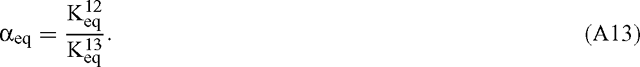
where αeq is the equilibrium isotope effect for aqueous CO2 / HCO3– given by (O’Leary 1981; Farquhar 1983; Farquhar et al. 1989; Brugnoli and Farquhar 2000):
This will be the case if the rate of reaction, r, is much greater than the instrument consumption rate, s, and so this simplification can be applied if enzyme concentrations are great enough that reactions are fast. In Fig. 2 (a typical MS trace), the initial reaction rate (after addition of RuBP) is ~40 times greater than the instrument consumption rate (before addition of RuBP) and so for membrane discriminations of the same order of magnitude as enzyme discriminations (or less), this simplification is valid and results in errors of less than 1‰. The equilibrium discrimination for dissolved bicarbonate relative to dissolved CO2 at 25°C is given by (Mook et al. 1974):

Guy et al. (1993) propose a similar correction factor, C, given by:

It should be noted that they have used the alternative definition for discrimination described by Eqns (A1) and (A2) so that C can be rearranged by substitution of Eqn (10):

C and αpart are essentially identical because the pKeq is substantially dictated by the dominant 12C isotope. They are also equivalent to the correction factor employed by Winkler et al. (1982). In terms of discrimination due to partitioning of inorganic carbon:

Now, in terms of the total or overall discrimination observed in the system:

Rearranging:

PEP carboxylase will have a different correction factor applied because it utilises bicarbonate as substrate, in which case:

Therefore:

At pH > 7, the correction factor is almost insignificant for PEPC because αpart and αeq are almost reciprocals owing to the fact that PEPC utilises the form of inorganic carbon (HCO3–) that is most prevalent. In terms of the total or overall discrimination observed in the system:

Rearranging:

Comparison of errors between different forms of the Rayleigh fractionation equation
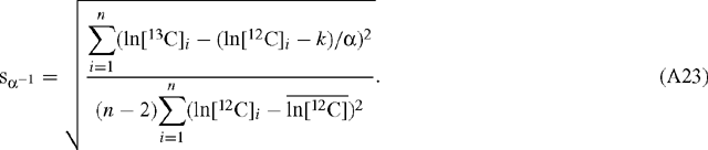
The standard linear regression algorithm is based on the assumption that there is no error in the abscissa value. This is avoided if the ‘least squares cubic equation’ is solved (York 1966). In order to apply standard linear regression, however, we need to determine whether or not the regressed slope and associated error is dependent on the choice of abscissa and ordinate. For a set of n measurements for ln[12C]i and ln[13C]i, where i denotes the ith measurement, standard linear regression with ln[13C] as the abscissa results in a value for α according to (Scott et al. 2004a):
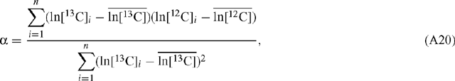
where  and
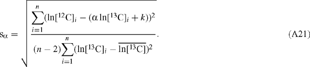
and  are the mean values of the natural logarithms of the signals for 12C and 13C, respectively (the regressed slope is independent of the amplification ratio for either signal). The standard deviation, s, of the slope estimate for α is (Scott et al. 2004a):
When ln[12C] is the abscissa:
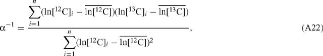
and:
The ratio of the scaled errors for α and α–1 is given by:
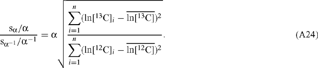
On average:

and so:

Hence the error is the same regardless of which of ln[12C] and ln[13C] is plotted as the abscissa and which as the ordinate. Linear regression of ln R v. ln[12C] results in a value for Δ′ according to:
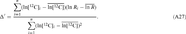
Now ln R = ln[13C] – ln[12C] and so:
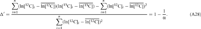
Hence, the slope estimates for α and Δ′ are equivalent and related as described in Eqn (10). The standard deviation of the slope estimate for Δ′ is:
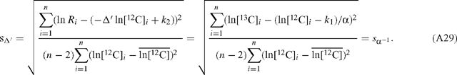
Therefore, the graphical method presented in this paper (ln[12C] v. ln[13C]) yields the same absolute error as the method used previously (ln R v. ln[12C]).