Evaluating a seasonal, sex-specific size-structured stock assessment model for the American lobster, Homarus americanus
Minoru Kanaiwa A C , Yong Chen A D and Carl Wilson BA School of Marine Sciences, University of Maine, Orono, ME 04469, USA.
B Maine Department of Marine Resources, Boothbay Harbor, ME 04575, USA.
C Current address: Department of Aqua-Bioscience and Industry, Tokyo University of Agriculture, 196 Yasaka, Abashiri, Hokkai, Japan 099-2493.
D Corresponding author. Email: ychen@maine.edu
Marine and Freshwater Research 59(1) 41-56 https://doi.org/10.1071/MF07121
Submitted: 28 June 2007 Accepted: 5 December 2007 Published: 25 January 2008
Abstract
Many models of different complexities are developed for fisheries stock assessment, and yet few have been rigorously evaluated for their performance in capturing fisheries population dynamics. This causes confusion about when a model should be used or not in assessing fisheries resources. This is especially true for models with complex structures. The present study evaluated the performance of a seasonal, sex-specific and size-structured stock assessment model with respect to the temporal pattern of recruitment, observation errors associated with input data, process errors and violation of model assumptions for the American lobster Homarus americanus. Using an individual-based lobster simulator, a series of lobster fisheries with different characteristics were simulated and the model was applied to the simulated data to estimate key fisheries parameters. Estimated values were then compared with the true values in the simulated fisheries to evaluate the model’s ability to capture the temporal trend in stock abundance, biomass and recruitment, and to identify factors that might result in model failure. Results show that this newly developed lobster stock assessment model performs well in capturing the dynamics of the lobster population under a wide range of conditions. Temporal trends in natural mortality and biased estimates of growth parameters posed the most serious problems. The present study shows the importance of model evaluation.
Additional keywords: model performance, population dynamics, simulation.
Acknowledgements
We would like to thank Atlantic States Marine Fisheries Commission (ASMFC) Lobster Model Development Subcommittee, Technical Committee and Stock Assessment Subcommittee for their support in the model development and testing. Comments from Dr L. Jacobson, Dr P. Breen, K. McKnown, J. Idoine, R. Glenn, Dr J. Wilson, Dr L. Mercer, Dr V. Crecco, P. Howell and S. Correia greatly improved the model. In particular, we are indebted to Dr L. Jacobson for his help and encouragement. We also would like to thank the ASMFC Lobster Model Peer Review Committee chaired by Dr R. Hilborn for their constructive comments, which greatly improved the early version of the model. Two anonymous referees and Dr A. Boulton are thanked for their useful comments on an earlier draft of this manuscript. Financial support of the work is provided by the Maine Sea Grant, Maine Department of Maine Resources, and ASMFC.
Breen, P. A. , Andrew, N. L. , and Kendrick, T. H. (2000). Stock assessment of PAU 5B for 1998–99. National Institute of Water and Atmospheric Research, Wellington, New Zealand. ,
Chen, Y. , Kanaiwa, M. , and Wilson, C. (2005). Developing and evaluating a Bayesian stock assessment framework for the American lobster fishery in the Gulf of Maine. New Zealand Journal of Freshwater and Marine Sciences 39, 645–660.
Fogarty, M. J. , and Idoine, J. S. (1988). Application of a yield and egg production model based on size to an offshore American lobster population. Transactions of the American Fisheries Society 117, 350–362.
| Crossref | GoogleScholarGoogle Scholar |
Kanaiwa, M. , Chen, Y. , and Hunter, M. (2005). Assessing stock assessment framework for the green sea urchin fishery in Maine, USA. Fisheries Research 74, 96–115.
| Crossref | GoogleScholarGoogle Scholar |
Palma, A. T. , Steneck, R. S. , and Wilson, J. (1999). Settlement-driven, multiscale demographic patterns of large benthic decapods in the Gulf of Maine. Journal of Experimental Marine Biology and Ecology 241, 107–136.
| Crossref | GoogleScholarGoogle Scholar |
Sheehy, M. R. J. (2001). Implications of protracted recruitment for perception of the spawner-recruit relationship. Canadian Journal of Fisheries and Aquatic Sciences 58, 641–644.
| Crossref | GoogleScholarGoogle Scholar |
Appendix 1: Description of the model
Recruitment model
Because of large variations among individuals, recruitment in a given year can come from up to seven year classes (Sheehy 2001). Previous studies suggested a weak stock-recruitment relationship. To avoid the potential problem, no functional relationship was assumed between spawning stock biomass (SSB) and subsequent recruitment in the present study. If we assume an average recruitment for all the years considered in the assessment is

where Rt is the recruitment for year t, Rdevt is the recruitment deviation from

and σRt is the standard deviation of the estimated recruitment for all the years included in the assessment and epst describes the part of the variation in Rt with the other part described by Rdevt – 1 of the previous year (Chen et al. 2005). Parameter Rh is an autocorrelation coefficient describing the degree of autocorrelations of recruitment of one year with the recruitment of the previous year. Its values range from 0 to 1, respectively, indicating no autocorrelation and perfect autocorrelation of the recruitment in years t and t – 1 (Breen et al. 2000). Recruitment only occurs in summer and fall, corresponding to major and minor molting events respectively. The minor molting occurs to a defined proportion of small individuals that have their second molt after the major molt.
Population dynamic model
Thirty-five size classes are defined, starting from 53 mm carapace length (CL) with a width of 5 mm. The choice of 5 mm for size class width is determined by the fact that the lobsters in most size classes have minimum molting increment of equal or larger than 5 mm (ASMFC 2000).
The lobster fishery started in 1800, but reliable information is not available from the early stages of the fishery. Thus we cannot treat the lobster as a virgin population for modelling. We need to estimate parameters that describe the size composition of the lobster stock in the first year defined in the assessment ( pik,1) and initial population size (Ni1), where i and k index sex and size class, respectively. The number of lobsters in size class k in the beginning of the first assessment season can be calculated as:

Initially, we directly estimated pik,1 (35 size classes for each sex, equivalent to 70 parameters to be estimated) and Ni1 (one parameter for each sex, equivalent to two parameters to be estimated; Chen et al. 2005). The ASMFC Lobster Model Peer Review Committee suggests using a log-normal density distribution function to describe pik,1. Thus, we have:


Equation (3c) is used to standardise the value of opik,1 calculated from the log-normal function in Eqn (3b) to ensure that the summation of pik,1 over all size classes is 1. This reduces the number of parameters to be estimated for pik,1 from 70 (Chen et al. 2005) to 4 (i.e. li and σi for females and males). Thus, six parameters need to be estimated for defining Nik,1 in Eqn (3a).
There is no evidence for sex-specific natural mortality before the first size class. Thus we assume a sex ratio of recruitment to the model of 0.5. The recruitment is equally divided among the first three size classes, considering the maximum increment in a molt can reach 16 mm. Thus, we have:

The pre-season total biomass, Bttotal, i, and pre-season legal biomass, Btlegal, i, in year t for sex i can be estimated as:


where wik is the weight of the lobster in size k, and Pk,t is a switch (0 for size classes below the minimum legal size or above the maximum legal size, and 1 for legal size classes). The exploitation rate, Uit, can then be calculated as:


where LCit is the landings in year t observed in the fishery measured in biomass (6a) or in number (6b). U in Eqns (6a) and (6b) is the biomass-based exploitation rate (Eqn 6a) and number-based exploitation rate (Eqn 6b).
No size impact is considered in calculating the overall exploitation rate using Eqn 6. The following approach was used for estimating the size-specific exploitation rate Uik,t. Considering various size-specific selectivity processes, the overall selectivity for lobsters of size k in time t, Sik,t, can be estimated as:

where Sk,tgear,i is the gear selectivity coefficient describing the proportion of lobster in size k, time t encountering and then retained in traps, Sk,tcons,i is the selectivity resulting from conservation measures such as V-notching and protection of egg-bearing lobsters, and describes the proportion of the lobsters in size k, sex i, and time t caught in traps, but thrown back to waters due to the conservation measures. Skother is the selectivity resulting from reasons other than gear selectivity, conservation measures and legal sizes for lobsters in size k to the fishery (Chen et al. 2005). The values of Sk,tgear,i and Sk,tcons,i are provided as input data (ASMFC 2000). The Skother is assumed to be invariant between sexes and over time, and follows a normal distribution function N(μS, σS2). The values of the normal distribution function are standardised to range from 0 to 1. The μS and σS2 determine the shape and location of the Skother and are parameters to be estimated in modelling. Because the overall selectivity Sik,t is the product of four selectivity coefficients and the legal switch has values of 0 and 1, the impacts of Sk,tgear,i, Sk,tcons,i and Skother on overall selectivity Sik,t are limited to lobsters of legal sizes (Sik,t is 0 for all other size classes because of Pk,t). The exploitation rate for lobsters of sex i in size class k in year t, Uik,t, can be calculated as:

where Uit is calculated from Eqn 6 (Chen et al. 2005). The exploitation rate derived in Eqn 8 is biomass-based if Uit in Eqn (6a) is used, and is abundance-based (i.e. number-based) if Eqn (6b) is used.
The survival rate from fishing, SVik,t, can then be calculated as:

The number of lobsters in size class k in year t, Nik,t, is calculated as:

where G is the size-specific growth transition matrix and M is the instantaneous rate of natural mortality. Natural mortality was assumed to consist of two components: natural mortality due to molting (M2) and average natural mortality resulting from all other natural causes (M1). Different natural mortality rates were assumed for different seasons to account for the seasonal difference in the lobster life-history process. The natural mortality rate for winter and spring was assumed to be M1. Because molting mainly occur in summer, natural mortality in summer was assumed to be M1 + M2. A proportion of lobsters that molt in summer also tend to molt in fall (ASMFC 2000). Thus the natural mortality for fall was assumed to be M1 + αM2, where α has a value between 0 and 1 for reflecting that only small proportion of lobsters tend to have second molt in a given year.
Because of the complexity of the framework, the growth transition matrix is determined outside the framework based on size-specific molting frequency and molting increment defined by the ASMFC Lobster Stock Assessment Subcommittee using an individual-based Lobster Simulator described in ASMFC (2006). Equation 10 is used in projecting the lobster population dynamics.
Model predictions
Using the above population dynamics models we can simulate a model lobster fishery. The following predictions can be made from the simulated model fishery.


where m indexes season, fishery catchability qi1,m is calculated as biomass-based:

or abundance-based:

where γ in Eqn 12 is a density-dependent parameter, and Eqns (12) implicitly assume that catchability differs among seasons and between sexes in the fishery and survey.


where Eqns (13a) and (13b) correspond to biomass and abundance-based survey indices, respectively, j ∈ {NMFS survey, DMR inshore survey and MA inshore survey in the present study} and survey’s catchability qi2,j,m can be calculated as:


and ψk,j in Eqn 13 is the proportion of lobsters in size class k that is covered by survey program j, and can be described by the following logistic curve:


In the simulation and application, we used the number (abundance)-based data in the parameter estimation.
Observational models
A group of observational models are developed to relate the predictions from the above dynamics models with the observations made in the fishery. The differences between the predicted and observed output variables in the observational models are assumed to be random and follow certain statistical distributions, which are then used to formulate the likelihood functions needed in the Bayesian parameter estimation. The following observational models are developed:


Error terms ϵ in Eqns 17 and 18 are assumed to follow normal distributions, and error terms ϵ in Eqns 19 and 20 are assumed to have multinomial distributions (Fournier et al. 1990).
Likelihood functions
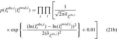
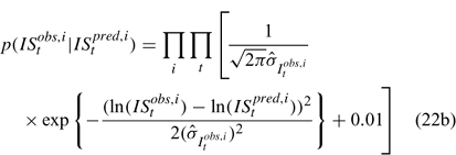
Three different likelihood functions used in Chen et al. (2000) are considered: (a) normal; (b) robust normal; and (c) t-distribution functions. The following likelihood functions are formulated based on the observational models listed above:


For the size composition data, a robust function (Fournier et al. 1990; Fournier 1996; Chen and Fournier 1999; Chen et al. 2000) described below is used,


