

Defining fire spread event days for fire-growth modelling
Justin Podur A C and B. Mike Wotton BA Faculty of Environmental Studies, York University, 109 Health, Nursing and Environmental Studies (HNES) Building, 4700 Keele Street, Toronto, ON, M3J 1P3, Canada.
B Natural Resources Canada, Canadian Forest Service, Faculty of Forestry, University of Toronto, 33 Willcocks Street, Toronto, ON, M5S 3B3, Canada.
C Corresponding author. Email: jpodur@yorku.ca
International Journal of Wildland Fire 20(4) 497-507 https://doi.org/10.1071/WF09001
Submitted: 7 January 2009 Accepted: 18 October 2010 Published: 20 June 2011
Journal Compilation © IAWF 2011
Abstract
Forest fire managers have long understood that most of a fire’s growth typically occurs on a small number of days when burning conditions are conducive for spread. Fires either grow very slowly at low intensity or burn considerable area in a ‘run’. A simple classification of days into ‘spread events’ and ‘non-spread events’ can greatly improve estimates of area burned. Studies with fire-growth models suggest that the Canadian Forest Fire Behaviour Prediction System (FBP System) seems to predict growth well during high-intensity ‘spread events’ but tends to overpredict rate of spread for non-spread events. In this study, we provide an objective weather-based definition of ‘spread events’, making it possible to assess the probability of having a spread event on any particular day. We demonstrate the benefit of incorporating this ‘spread event’ day concept into a fire-growth model based on the Canadian FBP System.
Introduction
Understanding and predicting the potential growth of forest fires is of both practical and scientific interest. Such predictions are used when planning initial attack and suppression operations. Fire-growth models, used to assess the spread of fire in a heterogeneous landscape, can also be used to assess the risk of fire at various points on the landscape when coupled with estimates of the probability of fire occurrence. Such models can then be used to assess the appropriateness of fuel treatment plans, including the creation of fuel breaks to reduce fire risk (Finney et al. 2007; Parisien et al. 2007). Accurate fire growth modelling is also important in understanding long-term, landscape-scale changes in fire frequency and intensity, as well as changes in landscape composition due to fire and forest succession interactions. For these reasons, fire-growth models that include an accurate representation of the linkages between fire weather, fuels and fire spread are crucial.
In Canada, forest fire management agencies use the Canadian Forest Fire Danger Rating System or CFFDRS (Stocks et al. 1989; Taylor and Alexander 2006) on a daily basis throughout the fire season to estimate forest fire potential. The CFFDRS consists of two major subsystems that each play specific roles in forest fire management operations. The Canadian Forest Fire Weather Index System or FWI System (Van Wagner 1987), used to assess fire danger, describes moisture in key forest-floor layers, and provides three fuel-type-independent relative indicators of potential forest fire behaviour. The moisture content of surface litter is characterised by the Fine Fuel Moisture Content (FFMC) and is important for determining the sustainability and vigour of surface fire spread (Lawson and Armitage 1997; Beverly and Wotton 2007). The moisture content of the upper portion of the organic layer in the forest floor is tracked by the Duff Moisture Code (DMC) and is important to sustainability of smouldering and fuel consumption in the forest floor (Van Wagner 1972a). The moisture content in deeper organic layers or in large pieces of woody debris on the forest floor is indicated by the Drought Code (DC), a useful indicator of extreme dryness and drought conditions that have the potential to make fire suppression more difficult and time-consuming. The system’s three relative indices of fire behaviour correspond to elements of Byram’s classic fireline intensity formula (Byram 1959): the Initial Spread Index (ISI) is a relative indicator of fire spread rate, the Build-up Index (BUI) is a relative indicator of the surface and ground fuel available for consumption and the FWI is a relative indicator of potential fire-line intensity (Van Wagner 1987).
The other main subsystem of the CFFDRS, the Fire Behaviour Prediction (FBP) System (Forestry Canada Fire Danger Group 1992), provides quantitative estimates of several key elements of fire behaviour: head fire rate of spread (ROS), fuel consumption and head fire intensity (HFI), using inputs such as fuels, topography, fire weather and fuel moisture (the latter based on FWI System outputs). The various models within the FBP System capture the key influences of environmental factors on fire behaviour; fuel-type-specific coefficients for these models are then statistically derived using observations made during extensive field experimental burning projects (e.g. Stocks 1987a, 1989; Alexander et al. 1991; Quintilio et al. 1991) in addition to well-documented wildfires. Although this reliance on observed data from large-scale field experimental burns limits the adaptability of the system to new fuel types, it allows the system to predict realistic rates of spread on wildfires, without arbitrary scaling factors. The FBP System provides such empirically based predictions of fire behaviour for 16 discrete fuel types found across Canada; these fuel types cover most of the important boreal forest stands, such as black spruce (Picea mariana), jack pine (Pinus banksiana), aspen (Populus tremuloides), and mixedwood stands consisting of aspen mixed with spruce or pine.
Experimental fires comprising the FBP System dataset were typically ignited in mid- to late afternoon, with the goal of documenting spread under peak burning conditions (Alexander and Quintilio 1990). In this respect, although fires were ignited by design over a range of conditions from marginal to high spread potential, the results tend to represent worst-case burning conditions. Fires were typically ignited as line fires at the edge of experimental plots (on a cleared fireline), with the goal of having a fire quickly achieve an equilibrium spread rate for the environmental conditions at the time of burn (Stocks 1987b). Because of the clearing of fireguard around the plot edges (Stocks 1987b), these ignition lines at the edges of plots likely had greater exposure to ambient winds than they would have had the ignition been carried out within a stand; observation of in-stand and fireline winds at an experimental burning project in jack pine in the North-west Territories of Canada support this conjecture (Table 3 in Taylor et al. 2004). In addition, when line ignitions in an experimental plot did not spread, these non-spread data points (essentially 0 m min–1 ROS) were not included in the final database used to develop the models in the FBP System; this would tend to lead to inflation of mean spread rates at the marginal or low end of spread potential. Consequently, we expect that, at the low to moderate fire spread potential end (e.g. surface fire spread in closed canopy forest), the FBP tends to overpredict average spread rate.
With the aid of a conceptual model of elliptical fire growth (Van Wagner 1969), the FBP System also provides estimates of flank and back fire rates of spread and fire shape as well as area and perimeter for a fire spreading in homogeneous fuels in unchanging weather conditions. The FBP System has been incorporated into several fire growth models throughout Canada. A cellular ‘contagion’ fire growth model was first described for Canada by Kourtz et al. (1977). Their model partitions a forest into grid cells, each of a single fuel type. Fire spreads from one grid cell to the next according to the rate of spread in the two cells and the wind direction. The spatial development of the fire through heterogeneous fuels, and under changing weather conditions, can thus be tracked over time. One implementation of this cellular growth model, WILDFIRE (Todd 1999), has been used in several landscape fire risk studies (Sanchez-Guisandez 2004; Espinoza 2005). Richards (1990) used an analogy with Huygens’ principle of wave propagation to develop a fire growth model that estimated fire spread over a short time period by treating the original fire perimeter as a set of ignition points from which the vertices of small individual elliptical wavelets propagate. The perimeter of the fire at the end of each short time step is then defined by a line that encloses each of these new wavelets. Finney (1998) combined Richards (1990), BEHAVE (Andrews et al. 2005), and the basic fire-spread models of Rothermel (1972, 1983) to develop a fire growth modelling platform, FARSITE, which has been used for operational fire behaviour analysis, planning and research. Finney (2002) later developed a more efficient algorithm to simulate fire growth, similar to that of Kourtz et al. (1977), based on minimum travel time methods. Finney showed that his algorithm generates results that are ‘essentially identical’ to simulated fire growth based on Huygens’ principle implemented in FARSITE. With fire behaviour in Canadian fuel types modelled by the FBP System, Richards’ (1990) wavelet propagation technique for fire growth was used to develop a fire growth modelling platform similar to FARSITE. This software platform, called PROMETHEUS (Tymstra et al. 2010), allows modelling of fire growth on heterogeneous landscapes (in terms of both fuels as well as topography) under time-varying weather conditions.
The FBP System and decision aids developed from it are well-accepted tools used for operational fire suppression throughout Canada. Because both the FBP and FWI Systems have been developed to provide indications of fire potential under the peak burning conditions of the day, various methods have been developed to ensure that these systems produce accurate predictions for the full range of fire behaviour and the full diurnal cycle. Lawson and Armitage (2008) discuss the implementation of the hourly FFMC (Van Wagner 1977) and the diurnal adjustment to the daily FFMC (Van Wagner 1972b; Lawson et al. 1996). Anderson (2009) compared the hourly FFMC calculation of Van Wagner (1977), the diurnal adjustment of Lawson et al. (1996) and the use of the Equilibrium Moisture Content (EMC). Each of these methods was used for both full 24-h days and also setting the FFMC to zero between sunset and sunrise (i.e. not allowing any spread at night). Each of the three methods studied by Anderson (2009) – hourly FFMC, diurnal adjustment and the EMC – has benefits and associated problems. Anderson (2009) found that the diurnal method of Lawson et al. (1996) combined with setting FFMC to zero at night produced the best predictions of fire growth, but argued that the EMC (combined with turning the calculations off at night) had the additional benefit of responsiveness to changes in hourly weather. The hourly FFMC of Van Wagner (1987) is also responsive to changes in hourly weather, but predicts much greater area burned than that observed (Anderson 2009). In the present paper, we offer a fourth method: the concept of a ‘spread event’.
Many fire managers categorise fire into days where the fire gets up and ‘runs’ and consequently increases in area, and days where the fire, although still active, is growing so slowly it can be assumed to not be increasing in size. On the latter days, suppression can have a major effect on a fire. The ‘spread event’ concept, combined with the hourly FFMC, can be viewed as another method for trying to produce accurate area burned predictions in fire growth modelling by adopting the simplifying assumption that fires grow during ‘spread events’ and do not grow on other days. A ‘spread event’ day is a day when the fire actively spreads (likely with high fire intensity) and adds a sizeable increment to the existing fire area. A ‘non-spread event’ is a day when the fire is still active and growing, but where conditions are such that spread rates, and subsequent growth, are very small and can be ignored in the overall growth history of the fire. This is a simplifying approximation – the rate of spread cannot be zero even on ‘non-spread’ days because the fire must still have an active perimeter or it would risk complete self-extinguishment. Anderson (2009) offers several possible reasons for the lack of observed growth (in reality) compared with the fire-growth model output, including the necessity of diurnal adjustments in litter moisture or the assumption in the model that the whole fire perimeter is active, when some of it, particularly flanks and rear, may have actually self-extinguished (Anderson et al. 2009). Here, we suggest another possibility: that these low-fire-potential periods may be due to what we have described here as a tendency for the FBP System to predict closer to ‘worst-case’ fire behaviour at the low end of fire potential, which could be corrected for by using the ‘spread event’ concept.
The benefit of the ‘spread event’ concept compared with the diurnal adjustment of Lawson et al. (1996), the hourly FFMC (Van Wagner 1977) or the EMC (Anderson 2009) is that it could be based on weather variables. If total area burned does depend on the number of ‘spread event’ days in the life of a fire, then predictions of future area burned, for example in climate-change scenarios, could be made more accurate if the weather associated with future ‘spread event’ days could be predicted from climate models.
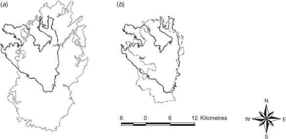
In attempting to model accurate fire growth on several historical fires in the boreal forest of the province of Ontario, Podur (2006) adopted a weather-based criterion for ‘spread event’ days and ‘non-spread event’ days based on an evaluation of the daily value of the ISI. A fire ‘spread event’ day was defined as a day when the daily ISI was greater than or equal to 7.5. On days when the ISI was below 7.5, the modelled fire did not grow (despite any small spread-rate predictions from the FBP System); on all other days, PROMETHEUS was used to model area burned. This ISI threshold value was chosen after consultation with Ontario Ministry of Natural Resources (OMNR) fire experts and used in that study to demonstrate the utility of the ‘spread event’ concept. Results from the fire growth analyses of a small subset of 11 large fires (where detailed perimeter and hourly weather information was available) found that it greatly improved the final fire size prediction. Fig. 1 shows an example of one of the fires analysed in Podur (2006): Chapleau-1–1999. Its actual final size was 19 745 ha. Without restricting spread to only those ‘spread event’ days, the predicted fire size was 53 154 ha, whereas using the spread event classification threshold of ISI ≥7.5, the predicted fire size was 22 180 ha. Another example fire from Podur (2006) was Dryden-10–2002, which had an actual final size of 1113 ha. Using PROMETHEUS to model each day simply with the observed hourly weather, the predicted fire size was 12 367 ha, but after limiting growth modelling to only those days matching the spread-event criteria, the predicted fire size was 1975 ha.
|
In this study, we developed and tested an objective weather (FWI)-based definition of ‘spread events’, making it possible to assess the probability of a ‘spread event’ on any particular day. We demonstrated the benefit of incorporating this ‘spread event’ day concept into an existing operational fire growth model (PROMETHEUS) based on the Canadian FBP System when modelling large fire growth over multiple days over a range of expected fire behaviour.
A forest fire may go through one or more single- or multiple-day periods when it is actively growing (spread events), with latent periods in between (non-spread events). We recognise that fire growth is a continuous process and temporal units of analysis of hours or even minutes could have been used, and that in fact ‘spread events’ could be merely hours or minutes long. However, we believe that there is merit in using this daily spread event concept to improve predictions made from fire-growth models, particularly in the case of landscape fire simulations.
There has been considerable interest in recent years in using satellite sensors for active wildfire detection and mapping in remote areas (e.g. Freeborn et al. 2009; Loboda 2009; Tekeli et al. 2009). For the current study, we chose a well-established existing product, hot spots from the MODIS (Moderate Resolution Imaging Spectroradiometer) Terra and Aqua satellites, to provide an objective classification of the days over the life of each fire into ‘spread events’ and ‘non-spread events’. MODIS has been used in numerous fire research studies (e.g. Pace et al. 2005; Giglio et al. 2006; Loboda 2009) and operational products exist to detect the locations of actively spreading fires in forests and rangeland around the world. We used information on active fires from the MODIS satellite to define spread events and non-spread events on individual fires. Next, we examined common fuel moisture codes and fire behaviour indices on these two types of event days to relate them to the active fires.
Methods
Fire and weather data
Fire management agencies in Canada keep records on fires that were suppressed in their jurisdictions. It is possible to compare these records with satellite records of active burning fires. Although each provincial agency operates independently, their fire reports all summarise numerous aspects of the fire’s history, including suppression activity it received. Such data include fire location, final area burned, weather, cause (lightning or people), and important dates in the fire’s history (start date, initial attack start date, being-held date, under control date, out – or extinguishment – date). We obtained fire report datasets for the years 2001 to 2006 for the province of Ontario from the OMNR.
We obtained daily archives of forest fire weather station observationsA and FWI System outputs for the same time period as our fire record for Ontario from the OMNR fire weather network consisting of more than 150 daily fire weather stations. The weather and FWI System codes and indices were then interpolated to the location of each fire, using a thin-plate cubic spline routine (Flannigan and Wotton 1989). This interpolation was carried out for each day from the start of a fire to the date the fire was declared out, resulting in a complete fire-weather record for each day of the fire’s growth.
Satellite hotspots: MODIS data
The MODIS archive of fire hot spots is a publicly available databaseB that gives daily locations (at a 1 × 1-km resolution) of the hot spots associated with fires that were actively spreading at the overpass time of the satellite. The MODIS sensors provide up to four thermal observations of the Earth’s surface in the mid- to high latitudes each day (at potentially any time of day). In Ontario, two of these passes typically occur (based on analysis of the datasets used in this study) throughout the afternoon (with typical passes at approximately 1300 and 1500 hours local time), well positioned to coincide with the period of active fire spread during the day. The MODIS methodology identifies as ‘active’ fires pixels with strong emission of mid-infrared radiation characteristic of fires (Giglio et al. 2003). Within a pixel, there is no way to differentiate between a small, intense fire and a less intense large fire.
Archives of MODIS hot-spot data were used to assemble hot-spot records from 2001 to 2006. These data were cross-referenced with the fire records to determine the active burning days of fires. Given the 1 × 1-km resolution of MODIS, this procedure underestimates the number of active spread days, especially for smaller fires. Despite this limitation, MODIS data can provide indication of when spread events occurred, particularly as more than 97% of the area across the Canadian landscape is burned by a relatively small number of larger (>200 ha) fires (Stocks et al. 2003).
A validation dataset
We used models developed in Ontario and assessed their accuracy using data from Alberta. We obtained forest fire, daily fire weather and fire danger rating records for 2001–06 for the province of Alberta from Alberta Sustainable Resource Development (ASRD). We also extracted hot-spot data for Alberta for the same period (2001–06) from the MODIS hot-spot archives.
Linking weather to MODIS hot spots
For each day between a fire’s start date and its end date, we joined fire weather and fire danger records with the daily MODIS hot-spot records. Hot-spot records were summarised to give a simple count of the number of hot spots (pixels) at the location of the fire on each day. If the satellite record showed one or more hot spots on a fire on a particular day, that day was classified as a ‘spread event’ day. Days without hot spots were classified as ‘non-spread events’. Thus we assume that the detection by MODIS of hot spots on a particular day is indicative of active, relatively high-intensity fire spread. Validations suggest that although MODIS may under-represent small and low-intensity fires, it is likely to detect high-intensity fires and consequently ‘spread events’ (Hawbaker et al. 2008; Roy et al. 2008).
Spread events and suppression
Because many of the fires were actively suppressed, we tried to eliminate bias due to suppression activity by only looking at the subset of days on which we were relatively confident the fire remained free-burning on some significant extent of its perimeter. For an actively crowning fire, intensities are typically such that direct suppression activity cannot limit the spread of the main fire front (if it in fact has any appreciable effect at all). Typically, in the suppression of a large fire on these active spread days, attack resources focus on the less-intense flanks and back fire, attempting to hold these while waiting for weather conditions to change to allow direct suppression on the head of the fire. Thus, one can expect that before the ‘being-held’ stage (termed BHE in Ontario, a label applied when the fire boss believes the fire will no longer grow significantly), even a fire being actively suppressed would add significant area on an active spread day. For our definition of a ‘spread event’, we are only concerned whether the fire was actively spreading and growing, not the extent of the growth; thus, we characterise a growth or non-growth day by only the presence or absence of hot spots on that fire on a particular day, not the number of hot spots detected. We believe that spread events are driven by weather conditions, which the fire suppression agency must respond to, and that while the agency can contain a fire between spread events (preventing further spread) and even reduce the area burned during some spread events, fire suppression activities will not likely stop a spread event from occurring on a fire with uncontained perimeter spreading through continuous fuels with the potential for spread. For fireline intensities greater than 4000 kW m–1, it is generally considered that direct suppression activity on the fire will not be successful (Alexander and Cole 1995). Therefore, we believe that between the start of a fire and the date the fire was declared BHE, suppression activity did not strongly influence our classification of ‘spread events’ and ‘non-spread events’. The decision to classify a fire as BHE, however, can sometimes be made conservatively, after suppression resources have contained a fire’s perimeter. We thus decided to only examine days between the start of the fire and the final growth day (as indicated by MODIS hot spot activity) before the BHE date. For fires in extensively protected areas, where fire growth is simply monitored without suppression activity, we examined days between the start date and the final ‘spread event’ before the declared ‘out date’. The final spread date in each of these situations is the de facto end of the fire. Our classification introduces a bias towards a higher probability of a spread event, because there may have been days when the fire could have spread but did not after our last ‘spread event’. These do not enter our dataset as zeros, because there is not yet an objective way to determine the end of a fire other than the fire agency’s necessarily conservative estimate of this date; this will be the subject of future work.
Logistic modelling
By choosing only fires with a final size greater than 10 ha, we obtained 2582 fire-days from the Ontario data, 773 of which were ‘spread event’ days and 1809 of which were non-spread days.
Logistic regression was used to model the probability of a ‘spread event’ day as a function of various potential predictors: observed daily fire weather, FWI System indices and codes, and FBP System outputs (HFI, ROS). We summarised means and medians of fire weather, and output codes and indices of the FWI System for each of the ‘spread event’ days and ‘non-spread event’ days to examine the differences of these distributions on each day. We summarised the mean and median ROS and HFI by estimating these values from the FBP System, assigning each fire to the C-2 (boreal spruce) fuel type. We chose to use the C-2 fuel type because boreal spruce is a common forest type throughout northern Ontario and in the FBP System represents a closed-canopy coniferous forest with ladder fuels in the understorey that aid in crown-fire development. Although the C-3 fuel type (mature Jack pine) is also a very significant presence throughout northern Ontario, for the high end of potential fire behaviour, ROS and HFIs predicted by the C-2 and C-3 models are very similar.
We graphically examined empirical relationships between the outputs of the FWI and FBP System and the probability of having a ‘spread event’ day by sorting our predictor variables into 15 to 20 subgroupings based on the numerical values of the variables. For example, for the ISI models, all data were grouped together into integer ISI ‘classes’, and ‘spread event’ days and ‘non-spread’ event days were totalled for each integer ISI class. An empirical value for probability of a ‘spread event’ day for each ISI class was then calculated by dividing the number of days with spread events at each ISI class by the total number of days in that ISI class. The relationships between empirical probability of a ‘spread event’ day and each variable were graphically examined.
We carried out a series of logistic regression analyses on those variables whose shift in distributions between spread and non-spread events made them candidates for an exploratory model. In these models, the dependent variable was a binary variable that classified each of the days in the life of the fire as either 0 for non-spread days, or 1 for days where significant spread occurred (as indicated by the presence of MODIS hot spots). Our goal was to develop a simple model that could be easily incorporated into fire-growth modelling, and to find the best single variable that provides a simple rule of thumb that could be readily applied in the field.
Validation data
Methods of associating fires, daily fire weather and fire danger and daily hot-spot information for the validation dataset in Alberta followed the same procedures as outlined above for Ontario. For this dataset spanning 2001 to 2006, we obtained 2383 fire-days, 568 of which were ‘spread event’ days. We used the logistic models developed in Ontario to classify days as either a potential spread day or non-spread day and then calculated measures of classification accuracy (i.e. accuracy, specificity) using observed spread events based on the MODIS records.
Results
Summaries of key weather and fire danger indices for ‘spread events’ and ‘non-spread events’ for Ontario (2001 to 2006) are provided in Table 1.C There is little difference between temperature and relative humidity (RH) between the two classes of days. The values change in the way one would expect (spread event days being warmer and less humid) though the change is quite small. In addition, and perhaps most surprisingly, wind speed, which one would expect would be a strong indicator of potential fire growth, does not seem to be different (in terms of its mean or median) between the two datasets. There appear to be strong differences between the means of most fire danger indices (perhaps excluding DC) as well as in the FBP System outputs.

|
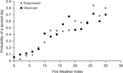
Fig. 2 shows empirical probability of spread event distributions for FFMC, ISI, BUI, FWI, ROS (C-2) and HFI (C-2). Each of the variables (which represent the stronger of the models based on logistic regressions) shows an ability to differentiate ‘spread events’ from ‘non-spread events’. Each of the points in these empirical plots represents a varying number of observations of spread and non-spread days at each fire danger variable class (i.e. the integer ISI values); typically, lower values of the fire danger variable classes are made up of averages of more points, as the distributions of these fire danger indices are typically right-skewed.

|
We used logistic regression (McCullagh and Nelder 1989) to examine whether the differences in the FWI System and FBP System outputs shown in Table 1 were in fact significant and, more importantly, useful for differentiating fire spread events from non-spread events. Coefficients defining the models and goodness-of-fit measures are shown in Table 2. Model fit is indicated by statistics summarising the percentage of concordant and discordant points, as well as the C statistic (concordance), which represents the overall association between modelled and observed outcomes. The final model form for predicting probability of a spread event is simply the logistic equation:

|

where A and B are constants and variable is the weather parameter or CFFDRS output being used as an indicator.
Each of the variables tested as a predictor of the occurrence of a spread day was statistically significant, with the exception of wind speed, which showed virtually no discriminatory power in the model. Both FFMC and hence ISI (despite the lack of wind signal) produced strongly significant models, but so too did DMC and BUI. FWI (which combines BUI and ISI) is a relative indicator of fire line intensity and produced a result similar to that of HFI from the FBP System. Basic fire weather observations (such as temperature and relative humidity), although they did produce significant relationships, did not perform as well as any of the FWI or FBP System outputs, with the exception perhaps of the DC, which also exhibited a weak signal.
To examine the effect of our assumption that before the BHE date, fire suppression did not affect the ‘spread event’ probability, we stratified data into fires with suppression activity and fires that spread unsuppressed and carried out the same logistic regression and graphical assessment of the probability of a ‘spread event’ day (Fig. 3). Including a simple binary categorical variable, ZONE, representing a suppressed fire (0) or an observed or unsuppressed fire (1) in the FWI-based model did not improve the fit of the model (model log likelihood = 426.9, Wald Chi-square for the ZONE variable = 1.03, P = 0.31). We also analysed the assumption that 10 ha was a lower limit of fire size that could be reasonably used; with the choice of a lower limit of 100 and 1000 ha, the comparison between the conditions on ‘spread event’ days and ‘non-spread event’ days was not different than the results presented here (though these limits did restrict the number of fires in the dataset).
|
Validation dataset
The Alberta dataset used for validation was summarised (Table 3) by ‘spread event’ day and ‘non-spread event’ day as was done for the Ontario dataset (Table 1). These summaries showed differences between ‘spread event’ and ‘non-spread event’ days similar to those we observed in Ontario. We used the Alberta dataset as a simple validation test case for the models we developed, and created simple 2 by 2 summary tables of success and failure of the predictions (a ‘confusion matrix’) using a probability of 0.5 as the model threshold for differentiating between a spread event and non-spread event. Table 4 shows these results for the strongest of the Ontario FWI, ROS and HFI models. Each of these models has virtually identical levels of accuracy, an indicator of the success of the model in predicting ‘spread event’ days and ‘non-spread event’ days correctly. The FWI-based model had the highest sensitivity; sensitivity is an indicator of what proportion of the actual positive values (spread events) the model predicted correctly.

|

|
Discussion
Podur (2006) used the ISI as a way of discriminating between ‘spread event’ days and ‘non-spread event’ days, choosing the threshold value of ISI = 7.5 suggested by OMNR fire experts for the C-2 FBP fuel type. The results in Table 2 show that ISI was a reasonable index for discriminating between these two growth types. Fig. 2b shows empirical probability of a spread event against ISI for the dataset used here, along with the model specified in Table 2. If we choose a probability value of 0.5 to differentiate between a spread day and non-spread day, then this corresponds to an ISI of 8.7. This is quite close to the expert opinion-based value used by Podur (2006) in his demonstration of the spread day concept. In our models, the Pspread = 0.5 cut-off for the HFI model is ∼9000 kW m–1, which is close to the 10 000 kW m–1 limit Alexander and Cole (1995) defined as representing ‘explosive’ fire behaviour that is nearly impossible to contain until burning conditions decrease.
The ISI, which combines the FFMC, an indicator of surface fuel moisture necessary for sustainable flaming, and wind speed, was originally expected to be one of the best single variables in terms of differentiating spread days from non-spread days. That DMC and BUI were as effective predictors of spread days indicates a significant signal from the consumption of heavier fuels, because both are indicators of the dryness of larger fuels and the consumption of those larger fuels and the forest floor. This significance of DMC (and consequently BUI) may indicate an effect of forest-floor consumption effectively raising surface-fire intensity and consequently raising the amount of crown engaged in flaming. It may also be a signal of the influence of surface organic layer moisture (as DC was not significant) on litter moisture content; such an effect was observed and quantified by Beverly and Wotton (2007).
Given the significance of ISI (an indicator of spread rate) coupled with the independent significance of BUI, it is logical that FWI (an indicator of fireline intensity – the combination of spread and fuel consumption) would be significant. FWI indeed produced a strong model in terms of likelihood ratio and C statistic (Table 2). The model based on FWI alone had similar (if not slightly better) model fit compared with the one based on rate of spread or HFI.
As many of the FWI and FBP System variables predict spread days well (Fig. 2), we recommend the FWI-based model, because it does not require the assumption of a fuel type, and the calculation of FWI itself is simpler than outputs of the FBP System, which are in fact based on FWI System outputs.
The absence of a correlation between wind speed and spread events was very surprising, because wind is a very well-established driver of fire behaviour (e.g. Rothermel 1972; Forestry Canada Fire Danger Group 1992; Cheney and Sullivan 1997). To investigate if this result was perhaps spurious and unique to our Ontario dataset, we carried out a logistic regression analysis of the influence of wind speed on probability of having a spread event using the Alberta validation dataset. The result was a marginally significant relationship (model log-likelihood –27.7, P < 0.0001, C statistic = 0.55). This low C statistic indicated very low concordance between model outputs and observations (a lack of concordance has a C statistic of 0.5) and a model with little to no predictive power. Furthermore, the sign of the wind coefficient in this weak relationship was negative, indicating the counterintuitive result that higher winds lead to lower probability of having a spread event.
There are several possible reasons for the lack of a relationship between wind speed and spread events. Winds for each fire do not represent a measurement at the location of the fire but values interpolated from the surrounding weather station network. Our analysis of potential interpolation error (using simple cross-validation techniques) showed that interpolation error is greater with wind speed than with temperature and RH, although these too can exhibit interpolation error, especially when the network is affected by passage of a weather front at observing time. In addition, wind varies on shorter time scales and less predictably than temperature or RH. Wind speeds observed at weather stations represent a single 10-min average taken at solar noon (this is the international standard), which may not be fully indicative of the winds that affect the fire during the spread event. Wind alone, without dry fuel, is not enough to cause a spread event. Our results thus suggest that daily interpolated wind values assigned to each fire may not be truly representative of the winds driving the fire spread.
Additional sources of potential error are related to the MODIS satellite data. First, MODIS is an infrared spectrometer and its observations can be obscured by clouds. This could result in missing spread events. This bias is reduced, however, because if there are clouds at overpass time, it is likely there was higher atmospheric humidity and a lower chance of high fire spread potential. Second, MODIS passes occur only four times per day over Ontario (twice per satellite), so some shorter spread events may have been missed.
There are several other possible refinements that could be made to the model to improve it. In addition to the standard weather variables (e.g. temperature, RH, wind speed) and FWI variables (e.g. FFMC, ISI), it is possible observations describing the vertical structure of the atmosphere at the fire location (e.g. atmospheric stability) or fuel-dependent variables (from the FBP System) might increase explanatory power or provide better fire-growth predictions. Fire spread and crowning potential, relevant in large fires that undergo spread events, are dependent on fuel type and structure. With all these caveats, however, we note that incorporating spread events using the simple models shown here improves fire-growth predictions dramatically, as discussed previously (Fig. 1).
Our model can be incorporated into fire-growth modelling in two ways. First, a simple rule of thumb could be used. If the probability of a spread day, Pspread = 0.5 is the threshold for defining a ‘spread event’ (though we do not suggest this is necessarily the proper threshold for defining a ‘spread event’ day), then this corresponds to an FWI of 19 or above (equivalent rules of thumb could be written for FFMC or ISI thresholds). This threshold value could be used as a rough guide by fire management personnel in the field, indicating a potential spread day if FWI is above this value and a non-spread day if it falls below.
A more sophisticated approach could be used for simulation. As the probabilistic model is available, random draws could be made from the probability of spread distribution to determine whether a day in the life of a fire was a spread day or a non-spread day. Using this approach with multiple replications, confidence intervals and error estimates for final size and even shape of fires could be calculated for fire-growth simulations.
Conclusions
Previous research found that, when using the PROMETHEUS wildland fire growth model (which relies on the FBP System), area burned estimates for the growth of large-fire spread over many days could be significantly overestimated. We combined MODIS satellite data on active fire growth with fire weather data to determine the weather conditions on days when fires grew significantly, or experienced a growth day. Using logistic regression, we found a strong relationship between many of the components of the FWI System (as well as weather parameters and FBP System outputs) and the occurrence of a ‘spread event’ day. The relationships we found can be used to improve the area burned predictions of fire-growth models when modelling the growth of a large fire over a multi-day period when weather is variable. Based on our results for Ontario, we recommend a simple model based on the FWI where a threshold of FWI > 19 defines the difference between a spread day and a non-spread day. Alternatively, the probabilistic model presented, which defines a spread day probability based on the FWI value, could be used in landscape fire modelling simulations. In future work, we will apply our model to fire-growth prediction for a series of well-documented fires. We will also develop a model for the probability of extinguishment, or of ‘fire-ending events’. Including both fire-ending events and spread events will further improve the accuracy and validity of fire growth models.
References
Alexander ME, Cole FV (1995) Predicting and interpreting fire intensities in Alaskan black spruce forests using the Canadian system of fire danger rating. In ‘Managing Forests to Meet People’s Needs: Proceedings of the 1994 Society of American Foresters/Canadian Institute of Forestry Convention’, 18–22 September 1994, Anchorage, AK. Publication 95–02, pp. 185–192. (Society of American Foresters: Bethesda, MD)Alexander ME, Quintilio D (1990) Perspectives on experimental fires in Canadian forestry research. Mathematical and Computer Modelling 13, 17–26.
| Perspectives on experimental fires in Canadian forestry research.Crossref | GoogleScholarGoogle Scholar |
Alexander ME, Stocks BJ, Lawson BD (1991) Predicting fire behavior in the black spruce–lichen woodland: the Porter Lake Project. Canadian Forest Service, Northern Forestry Centre, Information Report NOR-X-310. (Edmonton, AB)
Anderson KR (2009) A comparison of hourly Fine Fuel Moisture Code calculations within Canada. In ‘8th Symposium on Fire and Forest Meteorology’, 13–15 October 2009, Kalispell, MT. pp. 3A.4–3A.10. (American Meteorological Society: Boston, MA)
Anderson KR, Englefield P, Little JM, Reuter G (2009) An approach to operational forest fire growth predictions for Canada. International Journal of Wildland Fire 18, 893–905.
| An approach to operational forest fire growth predictions for Canada.Crossref | GoogleScholarGoogle Scholar |
Andrews PL, Bevins CD, Seli RC (2005) BehavePlus fire modeling system, version 4.0: user’s guide revised. USDA Forest Service, Rocky Mountain Research Station, General Technical Report RMRS-GTR-106WWW Revised. (Ogden, UT)
Beverly JL, Wotton BM (2007) Modelling the probability of sustained flaming: predictive value of fire weather index components compared with observations of site weather and fuel moisture conditions. International Journal of Wildland Fire 16, 161–173.
| Modelling the probability of sustained flaming: predictive value of fire weather index components compared with observations of site weather and fuel moisture conditions.Crossref | GoogleScholarGoogle Scholar |
Byram GM (1959) Combustion of forest fuels. In ‘Forest Fire: Control and Use’. (Eds KP Davis, A Brown) pp. 65–89. (McGraw-Hill: New York)
Cheney P, Sullivan A (1997) ‘Grassfires – Fuel, Weather and Fire Behaviour.’ (CSIRO Publishing: Melbourne)
Espinoza A (2005) Assessing the effects of FireSmart forest management strategies on the habitat for three wildlife species near Whitecourt, Alberta. MSc thesis, University of Toronto.
Finney MA (1998) FARSITE: Fire Area Simulator – model development and evaluation. USDA Forest Service, Rocky Mountain Research Station, Research Paper RMRS-RP-4. (Ogden, UT)
Finney MA (2002) Fire growth using minimum travel time methods. Canadian Journal of Forest Research 32, 1420–1424.
| Fire growth using minimum travel time methods.Crossref | GoogleScholarGoogle Scholar |
Finney MA, Seli RC, Mchugh CW, Ager AA, Bahro B, Agee JK (2007) Simulation of long-term landscape-level fuel treatment effects on large wildfires. International Journal of Wildland Fire 16, 712–727.
| Simulation of long-term landscape-level fuel treatment effects on large wildfires.Crossref | GoogleScholarGoogle Scholar |
Flannigan MD, Wotton BM (1989) A study of interpolation methods for forest fire danger rating in Canada. Canadian Journal of Forest Research 19, 1059–1066.
| A study of interpolation methods for forest fire danger rating in Canada.Crossref | GoogleScholarGoogle Scholar |
Forestry Canada Fire Danger Group (1992) Development and structure of the Canadian Forest Fire Behavior Prediction System. Forestry Canada Information Report ST-X-3. (Ottawa, ON)
Freeborn PH, Wooster MJ, Roberts G, Malamud BD, Xu WD (2009) Development of a virtual active fire product for Africa through a synthesis of geostationary and polar orbiting satellite data. Remote Sensing of Environment 113, 1700–1711.
| Development of a virtual active fire product for Africa through a synthesis of geostationary and polar orbiting satellite data.Crossref | GoogleScholarGoogle Scholar |
Giglio L, Descloitres J, Justice CO, Kaufman YJ (2003) An enhanced contextual fire detection algorithm for MODIS. Remote Sensing of Environment 87, 273–282.
| An enhanced contextual fire detection algorithm for MODIS.Crossref | GoogleScholarGoogle Scholar |
Giglio L, van der Werf GR, Randerson JT, Collatz GJ, Kasibhatla P (2006) Global estimation of burned area using MODIS active fire observations. Atmospheric Chemistry and Physics 6, 957–974.
| Global estimation of burned area using MODIS active fire observations.Crossref | GoogleScholarGoogle Scholar | 1:CAS:528:DC%2BD28Xksleqtbg%3D&md5=14c26f8104eb482b42732c154dd3cb09CAS |
Hawbaker TJ, Radeloff VC, Syphard AD, Zhu ZL, Stewart SI (2008) Detection rates of the MODIS active fire product in the United States. Remote Sensing of Environment 112, 2656–2664.
| Detection rates of the MODIS active fire product in the United States.Crossref | GoogleScholarGoogle Scholar |
Kourtz P, Nozaki S, O’Regan W (1977) Forest fires in the computer – a model to predict the perimeter location of a forest fire. Fisheries and Environment Canada, Information Report FF-X-65. (Ottawa, ON)
Lawson BD, Armitage OB (1997) Ignition probability equations for some Canadian fuel types. Final report submitted to the Canadian Committee on Forest Fire Management. (Ember Research Services Ltd: Victoria, BC)
Lawson BD, Armitage OB (2008) Weather guide for the Canadian Forest Fire Danger Rating System. Natural Resources Canada, Canadian Forest Service, Northern Forestry Centre, Catalogue No. Fo134-8/2008E-PDF. (Edmonton, AB)
Lawson BL, Armitage OB, Hoskins WD (1996) Diurnal variations in the Fine Fuel Moisture Code: tables and computer source code. Canadian Forest Service, Forest Resource Development Agreement Report 245. (Victoria, BC)
Loboda TV (2009) Modeling fire danger in data-poor regions: a case study from the Russian Far East. International Journal of Wildland Fire 18, 19–35.
| Modeling fire danger in data-poor regions: a case study from the Russian Far East.Crossref | GoogleScholarGoogle Scholar |
McCullagh P, Nelder JA (1989) ‘Generalized Linear Models.’ (Chapman and Hall: New York)
Pace G, Meloni D, di Sarra A (2005) Forest fire aerosol over the Mediterranean basin during summer 2003. Journal of Geophysical Research 110, D21202
| Forest fire aerosol over the Mediterranean basin during summer 2003.Crossref | GoogleScholarGoogle Scholar |
Parisien MA, Junor DR, Kafka VG (2007) Comparing landscape-based decision rules for placement of fuel treatments in the boreal mixedwood of western Canada. International Journal of Wildland Fire 16, 664–672.
| Comparing landscape-based decision rules for placement of fuel treatments in the boreal mixedwood of western Canada.Crossref | GoogleScholarGoogle Scholar |
Podur JJ (2006) Weather, forest vegetation, and fire suppression influences on area burned by forest fires in Ontario. PhD thesis, University of Toronto.
Quintilio D, Alexander ME, Ponto RL (1991) Spring fires in a semimature trembling aspen stand in central Alberta. Forestry Canada, Northern Forestry Centre, Information Report NOR-X-323. (Edmonton, AB)
Richards GD (1990) An elliptical growth model of forest fire fronts and its numerical solution. International Journal for Numerical Methods in Engineering 30, 1163–1179.
| An elliptical growth model of forest fire fronts and its numerical solution.Crossref | GoogleScholarGoogle Scholar |
Rothermel RC (1972) A mathematical model for predicting fire spread in wildland fuels. USDA Forest Service, Intermountain Forest and Range Experiment Station, Research Paper INT-115. (Ogden, UT)
Rothermel RC (1983) How to predict the spread and intensity of forest and range fires. USDA Forest Service, Intermountain Forest and Range Experiment Station, General Technical Report INT-143. (Ogden, UT)
Roy DP, Boschetti L, Justice CO, Ju J (2008) The collection 5 MODIS burned area product – global evaluation by comparison with the MODIS active fire product. Remote Sensing of Environment 112, 3690–3707.
| The collection 5 MODIS burned area product – global evaluation by comparison with the MODIS active fire product.Crossref | GoogleScholarGoogle Scholar |
Sanchez-Guisandez M (2004) FireSmart management of wildland/urban interface areas. MSc thesis, University of Toronto.
Stocks BJ (1987) Fire behavior in immature jack pine. Canadian Journal of Forest Research 17, 80–86.
| Fire behavior in immature jack pine.Crossref | GoogleScholarGoogle Scholar |
Stocks BJ (1987) Fire potential in the spruce budworm-damaged forests of Ontario. Forestry Chronicle 63, 8–14.
Stocks BJ (1989) Fire behavior in mature jack pine. Canadian Journal of Forest Research 19, 783–790.
| Fire behavior in mature jack pine.Crossref | GoogleScholarGoogle Scholar |
Stocks BJ, Lawson BD, Alexander ME, Van Wagner CE, McAlpine RS, Lynham TJ, Dube DE (1989) Canadian Forest Fire Danger Rating System – an overview. Forestry Chronicle 65, 258–265.
Stocks BJ, Mason JA, Todd JB, Bosch EM, Amiro BD, Flannigan MD, Martell DL, Wotton BM, Logan KA, Hirsch KG (2003) Large forest fires in Canada, 1959–1997. J. Geophysical Research 108, 8149
| Large forest fires in Canada, 1959–1997.Crossref | GoogleScholarGoogle Scholar |
Taylor SW, Alexander ME (2006) Science, technology, and human factors in fire danger rating: the Canadian experience. International Journal of Wildland Fire 15, 121–135.
| Science, technology, and human factors in fire danger rating: the Canadian experience.Crossref | GoogleScholarGoogle Scholar |
Taylor SW, Wotton BM, Alexander ME, Dalrymple GN (2004) Variation in wind and crown fire behaviour in a northern jack pine–black spruce forest. Canadian Journal of Forest Research 34, 1561–1576.
| Variation in wind and crown fire behaviour in a northern jack pine–black spruce forest.Crossref | GoogleScholarGoogle Scholar |
Tekeli AE, Sonmez I, Erdi E, Demir F (2009) Validation studies of EUMETSAT’s active fire monitoring product over Turkey. International Journal of Wildland Fire 18, 517–526.
| Validation studies of EUMETSAT’s active fire monitoring product over Turkey.Crossref | GoogleScholarGoogle Scholar |
Todd B (1999) User documentation for the Wildland Fire Growth Model and the Wildfire Display Program. Canadian Forest Service, Fire Research Network Report 37. (Edmonton, AB)
Tymstra C, Bryce RW, Wotton BM, Taylor SW, Armitage OB (2010) Development and Structure of PROMETHEUS: the Canadian Wildland Fire Growth Simulation Model. Natural Resources Canada, Canadian Forest Service, Northern Forestry Centre, Information Report NOR-X-417. (Edmonton, AB)
Van Wagner CE (1969) A simple fire-growth model. Forestry Chronicle 45, 103–104.
Van Wagner CE (1972) Duff consumption by fire in eastern pine stands. Canadian Journal of Forest Research 2, 34–39.
| Duff consumption by fire in eastern pine stands.Crossref | GoogleScholarGoogle Scholar |
Van Wagner CE (1972b) A table of diurnal variation in the Fine Fuel Moisture Code. Canadian Forest Service, Petawawa Forest Experiment Station, Information Report PS-X-38. (Chalk River, ON)
Van Wagner CE (1977) A method of computing Fine Fuel Moisture Content throughout the diurnal cycle. Canadian Forest Service, Petawawa Forest Experiment Station, Information Report PS-X-69. (Chalk River, ON)
Van Wagner CE (1987) Development and structure of the Canadian Forest Fire Weather Index System. Forestry Canada, Service Information Report ST-X-3. (Ottawa, ON)
A Fire weather in Canada is screen-level (2-m) temperature, relative humidity, 10-m open wind speed and direction, and 24-h accumulated precipitation all measured at 1300 hours Local Daylight Time (see Lawson and Armitage 2008).
B Data for this study were downloaded from http://modis.gsfc.nasa.gov/ and http://maps.geog.umd.edu/default.asp. Hotspots from fires active in 2002 were obtained from http://activefiremaps.fs.fed.us/canada/fireptdata/modisfire_2002_ca.htm. Methodology for hot-spot estimation and archiving is discussed at http://modis-fire.umd.edu/methodology.asp (websites last accessed 14 June 2010).
C Note that these fuel moisture and fire behaviour indices of the FWI System are designed such that increasing values indicate increasing levels of fire potential (e.g. an increase in FFMC indicates increasing dryness, despite that fact that it is an indicator of moisture).