

Representation and evaluation of wildfire propagation simulations
Jean-Baptiste Filippi A D , Vivien Mallet B C and Bahaa Nader AA Sciences Pour l'Environnement (SPE) and Centre National de la Recherche Scientifique (CNRS), University of Corsica, BP 52, F-20250 Corte cedex, France.
B Institut National de recherche en informatique et en automatique (INRIA), BP 105, F-78153 Le Chesnay cedex, France.
C Centre d'Enseignement et de Recherche en Environnement Atmosphérique (CEREA) (Ecole des Ponts ParisTech, Électricité De France (EDF) R&D; université Paris Est), 6–8 avenue Blaise Pascal, Cité Descartes Champs-sur-Marne, F-77455 Marne-la-Vallée, France.
D Corresponding author. Email: filippi@univ-corse.fr
International Journal of Wildland Fire 23(1) 46-57 https://doi.org/10.1071/WF12202
Submitted: 30 November 2012 Accepted: 30 May 2013 Published: 9 October 2013
Abstract
This paper provides a formal mathematical representation of a wildfire simulation, reviews the most common scoring methods using this formalism, and proposes new methods that are explicitly designed to evaluate a forest fire simulation from ignition to extinction. These scoring or agreement methods are tested with synthetic cases in order to expose strengths and weaknesses, and with more complex fire simulations using real observations. An implementation of the methods is provided as well as an overview of the software package. The paper stresses the importance of scores that can evaluate the dynamics of a simulation, as opposed to methods relying on snapshots of the burned surfaces computed by the model. The two new methods, arrival time agreement and shape agreement, take into account the dynamics of the simulation between observation times. Although no scoring method is able to perfectly synthesise a simulation error in a single number, the analysis of the scores obtained on idealised and real simulations provides insights into the advantages of these methods for the evaluation of fire dynamics.
Additional keywords: error, notation, score, scoring method.
Introduction
Model evaluation usually requires comparing predicted to observed values and is critical to establish potential errors and credibility (Appel et al. 2011). Forest fire propagation models have been developed for over 60 years. Originally these models provided a scientific method to determine a propagation speed that could easily be compared with observed rate of spread. The comparison only involved simple statistics. With the availability of computer simulation, fire growth models became available and required new scoring methods. A few specific or widely recognised mathematical or statistical methods were developed to evaluate their results (Fujioka 2002). However, defining scoring methods for such models is not straightforward, as there is a strong diversity in model’s intents and scales, as well as diversity in available observations.
Depending on their purpose, the forest fire models have been built to predict either the stationary zero-dimensional propagation speed (Rothermel 1972) or the full fire front evolution over time (Linn et al. 2002; Finney 2004). This paper focuses on models that can provide results at the scale at which the phenomenon is most usually observed (several hectares), e.g. Firestation (Lopes et al. 2002), Farsite (Finney 2004), ForeFire (Filippi et al. 2010) and many others that may be found in Sullivan (2009). It is important to note that using a scoring method will definitely not help to find the best model. All of these models have some kind of parameterisation and are sensitive to the quality of input data (e.g. wind, fuel). This set of methods can help to better estimate these parameters when observation is available. Error methods are also required to estimate a confidence level in case of perturbed ensemble simulations or model ensemble simulations.
Many scoring methods are readily available in the literature; most of these methods come from the field of image analysis or geophysics. A few of them have been specifically developed for fire models (Fujioka 2002). This paper focuses only on those that have been applied to forest fire simulation evaluation. If all these methods succeed in computing an error, they sometimes disagree and most of them are built to compare an observation to a simulation result at a given observation time, without taking into account the dynamical aspect of the observed and simulated fires. Moreover, a score is only applicable if it is compatible with operational forecast and takes into account the observation data available in that context.
Some reviews and investigations have been proposed for evaluation methods (Fujioka 2002), synthesised and extended by Finney (2000) in an internal report for the United States Department of Agriculture. The main conclusion is that it is very difficult (if not impossible) to synthesise simulation error in a single number and that a visual analysis provides a much better representation of the models performance for the trained analyst. We agree that trying to provide a model score for a limited set of observations of fire occurrence is not relevant to estimate model performance. Nevertheless, and much like Finney (2000), we believe that an analysis of a large dataset may be appropriate if it is possible to identify the necessary data and develop quantitative and objective tools to carry out the testing.
This paper provides a formal mathematical representation of a wildfire, reviews existing scoring methods using this formalism, proposes new methods and presents the associated tool that may be used to compute these scores. Using the proposed software, these methods are applied to synthetic simulation cases that are designed to expose their strengths and weaknesses. The methods are then tested for the simulation of two Mediterranean fires using observations that were available for the event. Finally, an overview of the software package is given, along with some recommendations about what method may be best appropriate to compare wildfires and to estimate simulation error.
Methods
Representation of a fire front and notation
This section focuses on the mathematical representation of the state of a firespread model seen as a dynamic model. In addition to the model’s state, other data is manipulated to carry out a wildfire simulation, such as elevation, fuel distribution and wind maps, but these datasets are neither a direct observation of a wildfire or prognostic results of the simulation. Fuel evolution over time (burned, suppressed, water quantity), fire area and fire surfaces are the typical data found in existing wildfire observation databases, even if available instruments do limit the quantity and quality of information that is available. After analysing the French Promethee database, the European EFFIS database and fire reports, one can note that different information levels, types and formats can exist in different forest fires data sources. A formal, mathematical representation of a forest fire must represent all this available information that can be divided in four levels.
For the simplest data, each event is composed of a time of occurrence, a scalar expressing the total area burned and an imprecise localisation (a location name or reference index in a low resolution grid used by firefighters). For the second level, the data are composed of one or many accurate ignition points, an ignition time and the final burned surface in the form of a polygon. In the third level of data, it is possible to find timely information about the evolution of the fire front over time, essentially the global fire perimeter over time, but also the time at which the fire reached specific locations (such as a road, a house, a ridge). Finally the most detailed data contains information about the actions performed by the firefighters and specific local information (e.g. flame height, intensity and spot-fire). Reports also often contain information about the wind, temperature and moisture evolution, but even if this information is important to simulate a wildfire, such information does not constitute a direct result of a wildfire propagation simulation to be evaluated.
No systematic file format exists for these datasets, but the relative simplicity of the first two levels make them easy to manipulate and transform. The data with the best quality and in the largest quantity is usually available in reports from the firefighters, with images and maps that must be manually processed in order to be digitally manipulated.
Mathematical notation required to formalise scoring methods must be able to represent the most complex available information.
Fire representation
Let t be the time and X the spatial position. We introduce the fuel consumption α(t,X) which is the ratio between the fuel mass available at t and position X, and the fuel mass initially available at X. It is set to 0 wherever no fuel has been burned yet, and to 1 where all of the fuel has been consumed. At locations where the fire is active, α(t,X) is between 0 and 1, depending on what proportion of fuel has been burned, relative to the amount of fuel initially available. For example, α(t,X) is 0.8 when 80% of the fuel initially available at X has been burned. Note that α(t,X) may also be in ]0,1[ at locations where the fire is not active anymore but did not burn all fuel. In locations where no fuel is available, no combustion can take place and α(t,X) is set to 0, for any t.
The front F(t) is defined as the closure of the region where the fuel is being burned at t: F(t) =
We identify the observed values with the exponent (superscript) o. For instance, the observed burned area at t is So(t).
Model’s state
In order to describe the full state of the model, the fuel consumption is needed as well as its time derivative that identifies the regions where the fire is active. The state of the system is thus defined as s(t,X) = (α(t,X),αY(t,X)).
Additional notation
We note |S| the area of the surface S. Using the Heaviside function H, defined so that H(x) = 0 if X ≤ 0 and H(x) = 1 if X > 0, we have |S(t)| = ∫ H(α(t,·)). We denote ∂S the boundary of S, and |∂S| the length of the curve ∂S.
We denote Ω the complete domain of interest. We assume that S(t), So(t) ⊂ Ω for any time t.
The simulation is run from t0 to tf , and the observed fire is active from to0 to at most tof where it is observed that the fire has stopped – note that the fire might have stopped earlier. Depending on the available information, tof may not be available. The final simulation time used to carry out the simulation can be: (1) the time tXf at which the simulated fire arrived to self-extinction – this is the only final time that can be used to forecast the final burned area, when observations are still unknown; (2) the time tof when the final observation is taken; (3) the time t=f at which the area of the simulated fire equals the area of the observed burned surface or (4) the time tf at which the simulated fire has the best agreement with the observations.
Review of error evaluation methods
Visual comparison has traditionally been the main means of comparing observed and simulated fire patterns. It appears that it is more relevant to compare fire front shapes over time than comparing fields because the phenomenon is active only at the interface between burned and unburned fuel. Because of this specificity, most methods applied to forest fire evaluation come from the fields of image analysis and geospatial statistics. Far from being exhaustive, this review tries to present several methods that have been employed to study forest fires.
Sørensen similarity index
Sørensen similarity coefficient (or Sørensen similarity index) is a statistical index, introduced in botany by Sørensen (1948). It computes the value (portion) of similarity between two samples. Perry et al. (1999) used this index to assess the agreement of fire simulation with observation.
Sørenson index specifically calculates the degree of inter-agreement between two sets. Here the two sets are the simulated and observed burned areas. Intersection of the two burned areas is divided by total burned areas. The result is a value between 0 and 1; 1 means a perfect agreement between observation and simulation, and 0 means there is no agreement. Sørenson similarity index is:
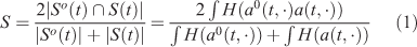
Score range: [0,1]
Best score: 1.
Jaccard similarity coefficient
Jaccard similarity coefficient was originally developed by Jaccard (1901). It is a statistical index similar to the Sørensen index.
Jaccard’s index is also a straightforward comparison method. The value is defined as the area of the intersection divided by the area of the union of the two sample sets (simulated and observed burned surfaces). The value ranges between 1 and 0, where 1 means perfect similarity between the two sets and 0 means disagreement. Jaccard similarity coefficient is:
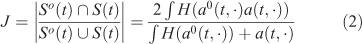
Score range: [0,1]
Best score: 1.
Kappa statistics
Kappa coefficients, which are statistical measures of agreement, have been developed by Cohen (1960). They have gained widespread use in assessing model-simulated vegetation distribution (Diffenbaugh 2003). In the field of forest fire error, kappa statistics have been used by Arca et al. (2007) for the estimation of the error of the Farsite simulator (Finney 2004) in a Mediterranean area. They have also been used to compare and detect changes in vegetation maps (Monserud and Leemans 1992).
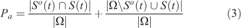
Cohen’s kappa coefficient is a statistical measure of inter-rater agreement for several categories and a method to classify the accuracy (Cohen 1960; Banerjee et al. 1999) that relies here on a cell by cell comparison between observed and simulated datasets to construct an error matrix. Kappa quantifies an overall agreement that is relative to the whole domain area minus possible random agreements (an overall probability that a region is either burned or unburned).
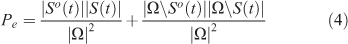
Relative agreement between two compared maps is estimated by:
Random agreement is calculated as:
After the probability of agreement by change is removed, the kappa coefficient reads:
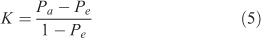
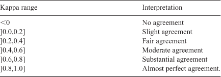
If kappa equals 1, there is a perfect agreement; if kappa equals 0, there is no agreement between simulated and observed fire maps. Negative values occur when agreement is weaker than expected but this rarely happens. Following Landis and Koch (1977), the interpretation of kappa values is provided in Table 1.
|
Ratio of areas
This method is a ratio of selected areas between observed and simulated fire shapes. It was introduced by Fujioka (2002). It describes the accuracy of agreement between two raster maps. The ratio of the areas is the sum of ratios between observed and simulated burned sector areas. In simple cases (like an ellipsoidal fire), the sectors divide the burned surfaces in portions that originate from the ignition. Each sector spans the region between the angles h and h+Δh, where the angle h is defined from a reference direction (usually north) and Δh represents the angular length of the sector. If the observed area is larger than the simulated area this ratio is greater than 1, so it must be divided by the union of the two areas.
Although this method can be used to estimate simulation error, it is important to note that it has been primarily designed to estimate local error in order to dynamically fit simulation parameters and to enhance simulation results that are obtained while the fire is running.
Let AΔhh be the simulated burned area of the sector between the angles h and h+Δh. Let AoΔhh be its observed counterpart. The ratio of the areas reads.
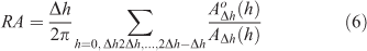
Score range: [0,+∞].
Best score: 1.
Note that the score can be equal to 1 even if the simulation is not perfect. Indeed, among the different angles, there can be compensations between ratios higher than 1 and lower than 1. Also note there may be large errors in directions where the front stayed close to the ignition point.
In case the burned surfaces are not convex, additional treatments should be carried out because the sectors are more complex to define. However, in this paper, we do not use these ad hoc corrections that depend on the simulated case that cannot be automated. As a consequence, the sectors all start from the ignition point.
Propositions of two new evaluation methods
The previous method may be automatically applied for simple shapes (ellipses or convex shapes) where a distance from the ignition point corresponds directly to a measure of the front propagation distance. Although this is usually true in constant fuel and topography conditions, this may not be the case with changing wind, complex terrain and heterogeneous fuels. Moreover, poor information about wind or ignition point might result in very similar, but rotated or translated shapes that may not necessarily represent a wrong behaviour of the simulation model. Kappa coefficients require the definition of an area of interest (evaluation domain), whereas others only take into account observed and simulated areas. The problem here is that there exists no formal way to determine the extent of the evaluation domain. As pointed out in Finney (2004), a simulation is also successful if it has effectively reproduced the area where fire has not been propagated (and observed).
Most previous methods compare an observed fire to a simulated fire at the same time (i.e. the observation time) (Arca et al. 2007). This creates a large dependency of the error on the observation time, which is often not precisely evaluated – even the fire duration is uncertain as it lies between an estimated fire ignition and some time when the fire is ‘fully extinguished’. In particular, these methods are unable to identify a simulation that would have provided a good or bad fire shape at intermediate times.
A general approach could be to keep the simulation running until the fire stops, and to compare final burned shapes, whatever the final observation and simulation times. The problem here is that fire simulation models are usually run with very poor information about the fire suppression events, and they often make use of stationary models for the rate of propagation (such as in the Rothermel model). Hence, there is no real final simulation time as simulation is likely to run until there is no more burnable fuel.
Another approach would be to compare the full simulation to one observation at some time, taking into account every intermediate state or step to provide a composite score. The arrival time agreement and shape agreement methods have been built to address these two issues. The first method is better suited to evaluate a simulation on a fully extinguished fire, whereas the second method may be better adapted to evaluate a running fire simulation.
Arrival time agreement
The arrival time agreement is based on the simulated arrival times (denoted T(X) at point X) and the observed arrival times To(X). Nevertheless, To(X) is usually unknown because observations are only available for a few times (sometimes just one, when the fire has stopped). When a burned surface is observed at time to, we set To(X) to to at all points X in the burned surface. Hence To(X) is an upper bound on the arrival time. If several burned surfaces are observed at different times, we set To(X) to the minimum time at which X is known to be burned.
We define the score at time to, which takes into account only the observations known at to. In practice, one will often choose to = tof, but the score is defined more generally for as.
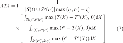
Score range: [0,1]
Best score: 1.
The score is composed of three integrals. The first one is the discrepancy between simulated and observed arrival times at locations burned in the simulation and in reality. When the difference T(X) – To(X) is negative, we cannot conclude that the simulated fire arrived too early because To(X) is an upper bound on the arrival time; hence the maximum time taken between T(X) – To(X) and 0. The second integral is for locations that were burned in the simulation but not in reality. This may because of early burning, with an advance in time of at least to– T(X). Similarly, the third integral is for locations that are not burned by the simulation at time tf so that the delay is at least tf – To(X).
If we know that to is greater or equal to tfo, any point in |S(tf)\So(to)| should never have been burned. In this case, we can replace the second term max(to – T(X), 0) with |tf – T(X)|.
Shape agreement
When an observed burned area So(to) is given for time to only, this observation provides some information about the other times: for times t < to, the area burned at t is included in So(to), and for times t < to , the burned area at t includes So(to). Consequently, whenever a simulation, whose exact dynamics are known, does not satisfy these conditions this should lead to some penalisation. Following this idea, we introduce the shape agreement over time that accumulates errors in time for the misplaced burned areas in the simulation:
The first term corresponds to the area burned in the simulation but not burned in reality until to. The second term corresponds to unburned areas in the simulation that are known to be already burned at to in reality.
Score range: [0,1]
Best score: 1.
This score can be extended for the case where there are several observations at different times to(1),…,to(n). If we denote in addition to(0) = max(t0,to0) and to(n+1) = tf, then the score reads.
where T = t(1)o – t(0)o + 2(t(n)o – t(n)o) + t(n+1)o – t(n)o.
If the fire is known to have stopped at or before, it is possible to add a term to penalise the overburned areas like ∫]tt(n),to(n+1)]|S(t)\So(to(n))|/|S(t)|dt.
Results and discussion
In this section, several tests are run in order to highlight the applicability, strengths and weaknesses of the different methods.
All tests are carried out using a description of the dynamics in the form of fields of arrival times. In Section, the methods are applied to evaluate simulations for two real forest fires. In Section, various synthetic cases are analysed so as to illustrate the behaviour of the scores in typical situations.
The results are illustrated with the maps of observed and simulated arrival times (Figs 1–7). In real cases, the observed arrival times are actually upper bounds on the arrival time as the burned surface cannot be observed continuously.
|
|
|
|
|
|
|
As the reader will notice, the scores magnitude of one method cannot be compared with the magnitude of another method. Also it is generally not possible to identify a threshold (for scores) that would indicate that a simulation is reliable or not. Instead, for one scoring method, the score values should be compared with each other so as to determine which simulation is the best. In other words, it is hard to state whether a model better simulated one fire than another, but a scoring method should help to rank the simulations for a given fire.
Synthetic cases
In this subsection, unless stated otherwise, the final simulation time tf is set to the final observation time tof.
Full error
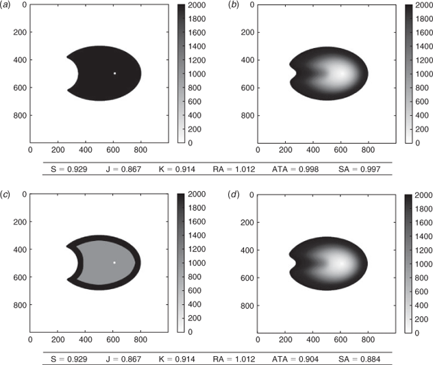
We consider the case where the simulation completely fails because the simulation ignition point is far from the real initial ignition point. The maps of arrival times and the score are reported in Fig. 1. Sørensen similarity index, Jaccard similarity coefficient and shape agreement are equal to zero and therefore clearly identify the simulation failure. The arrival time agreement is not zero, but it is very low compared with normal cases. The kappa coefficient is negative, which is consistent with the very poor agreement between the two burned surfaces. The ratio of areas could not be computed because the ignition points differ between the simulation and reality, so that the sectors could not be properly defined.
Dependence on domain size
In Fig. 2 we consider an isotropic fire propagation, with a simulation that is slightly faster than in reality. Two comparisons are made here, one with a large simulation domain and another with a smaller domain. We see that all scores remain identical, except the kappa coefficients which heavily depends on geographical distances in the map. One should consequently be cautious when using this indicator to compare the performance of different simulations that may not be run over the same domain.
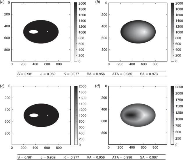
Erroneous shape with different dynamics
In this test (Fig. 3) the observed fire has propagated as an ellipse leaving an island of unburned fuel. We compare this to two erroneous simulations that burn the island. The first simulation propagates as a simple ellipse, without any specific change of speed over the island. The second simulation has different dynamics as the front first avoids the island and then burns it in the end. It is possible that this simulation burned the island too early. However its dynamics are more likely than that of the first simulation.
In both cases, the Sørensen similarity index, the Jaccard similarity coefficient, the kappa coefficient and the ratio of areas are identical. Indeed, they rely only on the final burned surfaces, which are the same in both cases.
On the contrary, the arrival time agreement and the shape agreement take into account the dynamics of the fire, and they can identify which simulation shows better agreement with reality. In the first simulation the island is burned early, which is highly inconsistent with the observations. The island is burned later in the second simulation, hence our two methods put less penalisation on the unduly burned island.
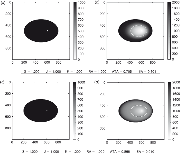
Arrival times
In this case (Fig. 4), the observed fire has propagated as a simple ellipse. The simulations also propagate as ellipses, but at the observed time they are both late; their burned surfaces are included in the observed burned surface. Until this time, the two simulations are associated with the same map of arrival times; indeed, their rates of speed have been identical.
Then, we let the simulations run so that tf = t=f, i.e. we let the simulations run until their burned areas are the same as the observed burned area. Right after tof, the first simulation is slower than the second simulation. The second simulation fills most of the observed burned area rather fast, whereas the first simulation takes more time. At the end of the simulation period, the first simulated fire expands faster compared with the second fire. Both simulated fires have burned the observed surface at the same final time tf. The difference is that, for a long time after tof, the second simulation has burned a larger area than the first simulation. Consequently, the second simulation is closer to the reality during this period. Its arrival time agreement and shape agreement are thus better than those of the first simulation.
On the contrary, the other scores fail to identify the best simulation. This is because of the fact that the two simulations are the same at tof and perfectly match the observed area.
Use of more observations
In Fig. 5, we compare the same simulated fire to two different observation sets of the same fire. The first observation set only contains the final burned surface and its time tof. The second observation set contains, in addition, one burned surface at an intermediate time.
The Sørensen similarity index, the Jaccard similarity coefficient, the kappa coefficient and the ratio of areas always give the same result as they are solely based on the final burned surface. On the contrary, the arrival time agreement and the shape agreement show different results that allow identification of the errors at the intermediate time. When compared to the final burned area, the final simulated area is erroneous, hence the scores are lower than 1. With the intermediate burned surface, we see that the simulated fire spread was first slower than in reality. In the observations, the fire expanded rather fast and then slowed down, which is not reproduced by the simulation. Consequently, introducing the intermediate observation should lower the evaluation scores, which is the case for the arrival time agreement and the shape agreement.
Real cases
This section presents two typical applications of the scoring methods. In the first application, the different scoring methods compare simulations with different stop conditions. In the second application, the results of models with different physical parameterisations are compared with observations consisting of burned surfaces at different times.
Contrary to previous results where both observations and simulations were synthetic, here the observations are field observations, and the simulations were carried out by the firespread model ForeFire (Filippi et al. 2010).
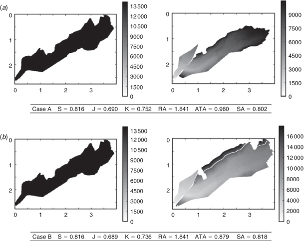
Suartone fire
The Suartone fire occurred in south-east Corsica on 28 July 2003 near the village of Suartone. About 456 ha were burned. The fire was detected at 1500 hours local time. This fire first spread moderately in an area surrounded by shrubs before it jumped a road, shifting on its right flank. As this flank was ~350–400 m wide, it became the fire head and accelerated driven by both a western wind and upslope effect. Finally, fire suppression action was taken on both flanks of the fire to control it and the fire ended its spread towards the sea ~1900 hours local time.
No quantitative information is available on the fire attacks and, depending on the model, the simulation may not extinguish the fire by itself. In this case, a condition must be found to stop the simulation. One option is to stop the simulation at the observed time, but this time may significantly maximise the actual fire extinction time. Most of the fire information available for reanalysis is in the same form, with a precise final contour but a final time that may be some time after the actual fire extinction.
In this test, two simulations were run from and with the same reference model, but until tf = t=f (i.e. until the simulation has reached the same area as the final observed area) in case A, and until tf = tXf in case B. The surface burned in case B is significantly larger than in case A. More details on the simulation settings for this case can be found in Santoni et al. (2011).
Sørensen, Jaccard and ratio of areas provide very similar, if not equal, scores in both cases because the effect on these scores of the overestimation in case B is equivalent to the effect of the underestimation in case A. Kappa coefficient gives a worse result for case B, because the overestimated area is large relative to the domain size. Likewise, arrival time agreement strongly penalises the overestimation in case B because the simulation burns significant areas long after the observed final time tof. On the contrary, shape agreement clearly favours case B as it strongly penalises the unburned area of case A after the early simulation end at tf = t=f.
Lançon-Provence fire
The Lançon-Provence fire took place in 2005 in the south of France and burned ~800 ha of shrubs and forest. On that day, a north-westerly wind was blowing, providing extreme propagation conditions. The fire started at 0940 hours local time and spread moderately until 1200 hours. Then the fire head gained intensity and propagated rapidly towards the south until it stopped ~1630 hours local time. In this case, the burned surface was recorded at different times during the ongoing fire, providing more observations than in the case of the Suartone fire. More details about the simulation setting for this case can be found in Filippi et al. (2010).
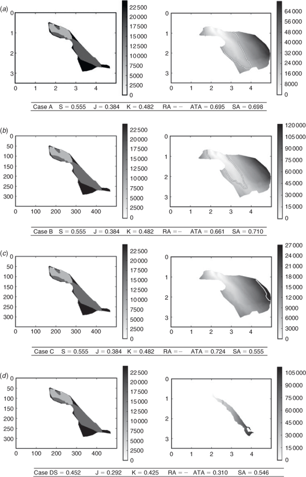
Several simulations of the Lançon-Provence case are run with different parameterisations. Case A is the reference simulation with the most likely (though highly uncertain) vegetation parameters for the day. In case B, the fuel height is divided by two, providing an overall slower propagation speed. In case C, the surface to volume ratio of dead fuel is multiplied by two, leading to a much faster propagation, in particular down wind. In case D, the surface to volume ratio is divided by two, constraining the fire to propagate down wind. The four simulations generated results with clearly different dynamics. All simulations were run until tf = tXf, so the simulation was expected to overestimate the burned area as fire attacks were not taken into account in the simulation. In the first three cases, all burnable vegetation was consumed up to the point that the fire reached a non-burnable vegetation, resulting in an identical final burned area but with very different fire dynamics.
The ratio of area method was not able to provide a score for any of these simulations because of the convex shape of the fire. Applying the method would have required manual relocation of the calculation points at certain simulation steps. Table 2 synthesises the case ranks according to the scoring methods. Sørensen, Jaccard and kappa scores give the same results for cases A, B and C because the final areas are identical in these three cases. The three scores find that case D is the worst simulation. Sørensen and Jaccard penalise the simulation more than kappa. Shape agreement and arrival time agreement provide very different results. Arrival time agreement strongly penalises under-prediction, i.e. strongly penalising a fire that missed burned areas. Consequently, case C is marked as the best simulation, as it manages to never underestimate burned area (all simulations except C underestimated the burned area at the south of the fire). Case A is the next best score for arrival time agreement, followed by case B and a much lower score for case D that strongly underestimates burned areas.
|
Shape agreement method is a stronger marker of overall shape accordance and ranks case B as the best simulation, with a close case A. This ranking is due to the fact that the case B (slower) underestimations of the southern part of the fire are slightly lower than case A (quicker) overestimations of the northern part of the fire. Overall these two scenarios provide the shapes that are most similar to the observation at t = tof. As shape agreement is equally penalising under- and over-prediction, the scores are about the same for cases D and C – case D under predicts about as much as C over predicts.
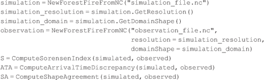
Software
The scoring methods have been implemented in a Python library with minimum dependencies. It is available at http://sourceforge.net/projects/pyfirescore/ (accessed 12 July 2013). It relies on NumPy (Oliphant 2006) and SciPy (Jones et al. 2001). The base format for forest fire simulation and observation is NetCDF, with a fire data convention such as proposed by Nader et al. (2011). If the information is not directly available as a well formated NetCDF file, it is possible to import data as bitmap image, points list or matrices in different file formats and encoding. Such imports can be scripted and can benefit from the numerous input/output libraries already available for Python. Below is a commented example of score computations with the library.
|
The previous lines first load simulated data from a NetCDF file. The spatial resolution of the simulation grid (i.e. the grid corresponding to the matrix of arrival times) and its extent are retrieved, so that the observations can be mapped to this grid. Once the simulation and the observations are loaded, a single call to a function carries out the score computation.
Conclusion
This paper has reviewed a set of evaluation methods and proposed two new evaluation scores, using formal notation. A software tool is provided along with the paper so that a Python implementation of the methods is available to the reader.
A set of synthetic cases was built in order to illustrate the differences and advantages or drawbacks of all methods. The paper stressed the importance of scores that can evaluate the dynamics of the model, as opposed to methods relying on snapshots of the burned surfaces computed by the model.
The analysis of scores obtained on idealised and real cases demonstrates some advantages of the dynamics-aware methods. However, it appears that no scoring method is able to perfectly synthesise a simulation error in a single number. The two proposed methods seem more appropriate if one wants to specifically evaluate the quality of the simulation dynamics. These methods can always be applied when the simulation arrival times or intermediate simulated fronts are recorded in the course of the simulation. Therefore, we recommend, whenever possible, to compute either the arrival time agreement or the shape agreement. In addition, these scores can be seamlessly applied with one final observed surface or with several intermediate observed burned surfaces. They always evaluate the whole simulation, from its ignition to its extinction.
The availability of efficient evaluation methods can help to couple simulation models and observations. There is indeed a need for sound comparison between model states and observations if one wants to apply data assimilation algorithms, like a Kalman filter (Beezley and Mandel 2008) or the four-dimensional variational assimilation.
The methods described in this paper are adapted to the evaluation of one model, for one simulation. However, a reliable evaluation of modelling system should involve several simulation cases and maybe an ensemble of simulations. This is especially true when dealing with large fires, propagating during several days, where the complexity of the propagation makes it very difficult for one model to represent the diversity of the events. The ensemble of simulations could be made of perturbed simulations with the same model or with simulations from different propagation models. This would require different comparison scores, but probably based on the dynamic-oriented approaches of this paper. These composite scores, relevant for probabilistic forecasts and risk assessment, should be the subject of future research.
Acknowledgements
This research is supported by the Agence Nationale de la Recherche, project ANR-09-COSI-006 IDEA. The authors thank Marc Finney who helped to define the problem and the anonymous reviewers for their comments on this work.
References
Appel KW, Gilliam RC, Davis N, Zubrow A, Howard SC (2011) Overview of the atmospheric model evaluation tool (AMET) v1.1 for evaluating meteorological and air quality models. Environmental Modelling & Software 26, 434–443.| Overview of the atmospheric model evaluation tool (AMET) v1.1 for evaluating meteorological and air quality models.Crossref | GoogleScholarGoogle Scholar |
Arca B, Duce P, Laconi M, Pellizzaro G, Salis M, Spano D (2007) Evaluation of {FARSITE} simulator in Mediterranean maquis. International Journal of Wildland Fire 16, 563–572.
| Evaluation of {FARSITE} simulator in Mediterranean maquis.Crossref | GoogleScholarGoogle Scholar |
Banerjee M, Capozzoli M, McSweeney L, Sinha D (1999) Beyond kappa: a review of interrater agreement measures. The Canadian Journal of Statistics/La Revue Canadienne de Statistique 27, 3–23.
| Beyond kappa: a review of interrater agreement measures.Crossref | GoogleScholarGoogle Scholar |
Beezley JD, Mandel J (2008) Morphing ensemble Kalman filters. Tellus 60A, 131–140.
Cohen J (1960) A coefficient of agreement for nominal scales. Educational and Psychological Measurement 20, 37–46.
| A coefficient of agreement for nominal scales.Crossref | GoogleScholarGoogle Scholar |
Diffenbaugh NS (2003) Vegetation sensitivity to global anthropogenic carbon dioxide emissions in a topographically complex region. Global Biogeochemical Cycles 17, 1067
| Vegetation sensitivity to global anthropogenic carbon dioxide emissions in a topographically complex region.Crossref | GoogleScholarGoogle Scholar |
Filippi J-B, Morandini F, Balbi JH, Hill DR (2010) Discrete event front-tracking simulation of a physical fire-spread model. Simulation 86, 629–646.
| Discrete event front-tracking simulation of a physical fire-spread model.Crossref | GoogleScholarGoogle Scholar |
Finney MA (2000) Efforts at comparing simulated and observed fire growth patterns. USDA Forest Service, Rocky Mountain Research Station, Technical Report INT-95066-RJVA. (Missoula, MT)
Finney MA (2004). Farsite: fire area simulator-model development and evaluation. USDA Forest Service, Rocky Mountain Research Station, Technical Report RMRS-RP-4. (Missoula, MT)
Fujioka FM (2002) A new method for the analysis of fire spread modeling errors. International Journal of Wildland Fire 11, 193–203.
| A new method for the analysis of fire spread modeling errors.Crossref | GoogleScholarGoogle Scholar |
Jaccard P (1901) Étude comparative de la distribution florale dans une portion des Alpes et des Jura. Bulletin de la Société Vaudoise des Sciences Naturelles 37, 547–579.
Jones E, Oliphant T, Peterson P, et al. (2001). SciPy: open source scientific tools for Python. Available at http://www.scipy.org/ [Verified 14 June 2013]
Landis JR, Koch GG (1977) The measurement of observer agreement for categorical data. Biometrics 33, 159–174.
| The measurement of observer agreement for categorical data.Crossref | GoogleScholarGoogle Scholar | 1:STN:280:DyaE2s7jsFWqtA%3D%3D&md5=2b13c5be704ad8bc2e29c6e168bc550bCAS | 843571PubMed |
Linn R, Reisner J, Colman JJ, Winterkamp J (2002) Studying wildfire behavior using FIRETEC. International Journal of Wildland Fire 11, 233–246.
| Studying wildfire behavior using FIRETEC.Crossref | GoogleScholarGoogle Scholar |
Lopes A, Cruz M, Viegas D (2002) Firestation – an integrated software system for the numerical simulation of fire spread on complex topography. Environmental Modelling & Software 17, 269–285.
| Firestation – an integrated software system for the numerical simulation of fire spread on complex topography.Crossref | GoogleScholarGoogle Scholar |
Monserud RA, Leemans R (1992) Comparing global vegetation maps with the Kappa statistic. Ecological Modelling 62, 275–293.
| Comparing global vegetation maps with the Kappa statistic.Crossref | GoogleScholarGoogle Scholar |
Nader B, Filippi JB, Bisgambiglia P-A (2011) An experimental frame for the simulation of forest fire spread. In ‘Proceedings of the 2011 Winter Simulation Conference’, 11–14 December 2011, Phoenix, AZ. (Eds S Jain, RR Creasey, J Himmelspach, KP White, M Fu) pp. 1010–1022. (IEEE)
Oliphant TE (2006) ‘Guide to NumPy.’ (Trelgol Publishing: USA) Available at http://www.numpy.org [Verified 29 August 2013]
Perry GLW, Sparrow AD, Owens IF (1999) A {GIS-supported} model for the simulation of the spatial structure of wildland fire, Cass Basin, New Zealand. Journal of Applied Ecology 36, 502–518.
| A {GIS-supported} model for the simulation of the spatial structure of wildland fire, Cass Basin, New Zealand.Crossref | GoogleScholarGoogle Scholar |
Rothermel R (1972) A mathematical model for predicting fire spread in wildland fuels. USDA Forest Service, Intermountain Forest and Range Experiment Station, Research Paper INT-115. (Odgen, UT)
Santoni P, Filippi JB, Balbi J-H, Bosseur F (2011) Wildland fire behaviour case studies and fuel models for landscape-scale fire modeling. Journal of Combustion 2011, 613424
| Wildland fire behaviour case studies and fuel models for landscape-scale fire modeling.Crossref | GoogleScholarGoogle Scholar |
Sørensen T (1948) A method of establishing groups of equal amplitude in plant sociology based on similarity of species and its application to analyses of the vegetation on Danish commons. Biologiske Skrifter 5, 1–34.
Sullivan AL (2009) Wildland surface fire spread modelling, 1990–2007. 3. Simulation and mathematical analogue models. International Journal of Wildland Fire 18, 387–403.
| Wildland surface fire spread modelling, 1990–2007. 3. Simulation and mathematical analogue models.Crossref | GoogleScholarGoogle Scholar |