

Short-term fire front spread prediction using inverse modelling and airborne infrared images
O. Rios A , E. Pastor A B , M. M. Valero A and E. Planas AA Department of Chemical Engineering, Centre for Technological Risk Studies, Universitat Politècnica de Catalunya – BarcelonaTech, Diagonal 647, E-08028 Barcelona, Catalonia, Spain.
B Corresponding author: Email: elsa.pastor@upc.edu
International Journal of Wildland Fire 25(10) 1033-1047 https://doi.org/10.1071/WF16031
Submitted: 23 February 2016 Accepted: 14 July 2016 Published: 3 October 2016
Journal Compilation © IAWF 2016
Abstract
A wildfire forecasting tool capable of estimating the fire perimeter position sufficiently in advance of the actual fire arrival will assist firefighting operations and optimise available resources. However, owing to limited knowledge of fire event characteristics (e.g. fuel distribution and characteristics, weather variability) and the short time available to deliver a forecast, most of the current models only provide a rough approximation of the forthcoming fire positions and dynamics. The problem can be tackled by coupling data assimilation and inverse modelling techniques. We present an inverse modelling-based algorithm that uses infrared airborne images to forecast short-term wildfire dynamics with a positive lead time. The algorithm is applied to two real-scale mallee-heath shrubland fire experiments, of 9 and 25 ha, successfully forecasting the fire perimeter shape and position in the short term. Forecast dependency on the assimilation windows is explored to prepare the system to meet real scenario constraints. It is envisaged the system will be applied at larger time and space scales.
Additional keywords: data assimilation, fire behaviour, Rothermel model.
Introduction
Wildfire phenomena constitute a widespread problem that causes human, environmental and economic losses all over the world every year. One of the key aspects to reduce their impact is to improve and optimise wildfire-fighting capacities by providing the emergency responders with sound information on the upcoming wildfire dynamics. However, the accuracy of the current available operational wildfire models such as FARSITE (Finney 1998) or PHOENIX Rapidfire (Tolhurst et al. 2008) is limited owing to the scarcity of precise data available to initialise them (Finney et al. 2013) and the empirically developed submodels that they contain (Sullivan 2009), which make them unsuitable to be exported to all sorts of different fire events. An alternative approach to wildfire modelling is computational fluid dynamics (CFD)-based models such as FIRETEC (Linn 1997), FOREFIRE (Filippi et al. 2009; Filippi et al. 2014a) or Wildland–Urban Interface Fire Dynamics Simulator (WFDS) (Mell et al. 2007). However, these are restricted to research use, and small- and particular-scale applications owing to the high computational costs and initialising data required (Viegas 2011). A simplified version of a CFD model that couples weather modelling with Rothermel’s fire-spread model (Rothermel 1972) named WRF-SFIRE (Mandel et al. 2014, 2011) was recently reported to have been applied operationally, as a 6-h forecast could be launched with a 30-min run in a multicore processor.
Cruz and Alexander (2013) reviewed 49 fire spread models datasets and found that only 3% of the simulations acceptably predicted the observed rate of spread (RoS) and revealed the need to adjust those models if they were to be used operationally. To deal with this problem, data assimilation has shown great potential to correct a model’s predictions. Mandel et al. (2009) pioneered the use of data assimilation for wildfire modelling, predicting flame temperature and location using an ensemble Kalman filter framework and an atmosphere-coupled wildfire model. Their work showed promising results while raising some concerns about spurious fire corrections and the computing time required. Following their idea, Rochoux et al. (2014a, 2014b, 2015) explored a data-driven wildfire simulator based on parameter and state estimation that assimilates fire front positions and corrects the wildfire forecast by means of a level set model based on Rothermel’s. They explored a parameter and state estimation strategy with stochastically based estimation of the error covariance matrices. The simulator was run using parallel computing and showed great capacity both in synthetically generated data and a small-scale controlled experiment. Lautenberger (2013) also used Rothermel’s model and a data-assimilating approach to calibrate fire propagating parameters to meet observed fire shape. All these authors used an Eulerian level set method to track fire front propagation. Although this approach offers advantages when dealing with crossovers and large perimeters, it also has some drawbacks such as the level set solution dependency on the mesh (Mallet et al. 2009) and the requirement of a flux limiter to filter fire front shapes (Bova et al. 2016).
The alternative approach to propagate the front is the Lagrangian framework, which tracks front markers individually. This approach has been successfully applied on most broadly used fire simulators (FARSITE (Finney 1998), Phoenix RAPIDFIRE (Tolhurst et al. 2008), or PROMETHEUS (Tymstra et al. 2010) as an example). The final front shape equivalence of both approaches was recently demonstrated by Bova et al. (2016) over complex topographical domains.
Some authors also worked to couple Lagrangian-based fire models with data assimilation. Denham et al. (2012) successfully applied genetic algorithms (GA) to find the wind configurations that best resemble observations to launch an improved forecast. A combination of weather and fuel calibration using fire perimeters has also been implemented using FARSITE (Finney 1998) and high-performance computing, showing great improvements and potential for long-term predictions (Wendt et al. 2011; Artés et al. 2014). Combining these ideas, Rios et al. (2014) developed a data-driven algorithm based on Rothermel’s RoS model (Rothermel 1972) and Huygens’ elliptical propagation (Richards 1990; Glasa and Halada 2008) and proved that it provides a short-term highly accurate forecast of wind-driven wildfires when tested with synthetically generated data.
In the present work, we further develop this algorithm to cope with real wildfire data to produce a reliable short-term forecast. We test it by assimilating airborne infrared images captured from two large-scale experiments conducted in South Australia (Cruz et al. 2013) and assess the forecast reliability by means of Jaccard (Jaccard 1901; Filippi et al. 2014c) and Sørensen (Sørensen 1948; Perry et al. 1999) similarity indices, finding great agreement in the available short-term forecast.
The paper is organised as follows: the Methods section presents the complete algorithm rationale and description of real-scale experiments used for validation. The algorithm performance is explored in depth in the Results and discussion section where the forecasting capabilities and system parameters are investigated and discussed. Finally, we provide some concluding remarks and an outline of proposed future work.
Methods
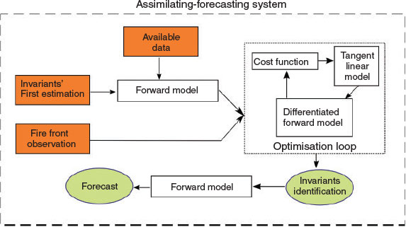
Our system combines two main sequential tasks that are envisaged to take place cyclically. The first one involves solving an inverse fire modelling problem by which the parametric space of certain observed fire front behaviour is found. This approach is based on the assumption that there are several variables that remain constant during a certain period of time, and thus we call them invariants. These invariants can be either physical quantities or unknown model parameters that determine the fire front dynamics. With the aid of a proper assimilation framework, these invariants can be resolved using the available data (e.g. fuel characteristics, topography, weather conditions) to reproduce certain fire behaviour observations (i.e. fire perimeters sensed by airborne IR). The second task involves launching a forecast with the forward fire behaviour model, relying on the corrected invariants, which are then entered as input back into the model to deliver a more accurate forecast. The algorithm begins with the input of the observed fire front isochrones, the complementary available data and initialisation of the invariants. Then, an optimisation loop identifies the proper invariants that best suit the fire dynamics observed, and these are finally used to launch the forecast. The algorithm flow is depicted in Fig. 1 and shows the key aspects that will be explained in detail in the following sections.
|
Algorithm rationale
Forward model
The first key aspect of the overall system is the forward model. The forward model is the mathematical model that allows one to explain the phenomenon and exhibits a capacity to reproduce the assimilated wildfire dynamics. To be suitable for an operational inverse-modelling scheme, the forward model has to be computationally efficient to ensure the forecast is delivered before the event takes place (i.e. positive lead time). While keeping options open to explore further models, in the present work, we chose a model based on Rothermel (Rothermel 1972) to determine RoS and a Huygens’ expansion-based approach to propagate the front in 2D (Richards 1990, 1993). The Rothermel model (see Eqn 1) is based on a simple energy balance that expresses the fire heat source by means of the reaction intensity ( ), the propagating flux ratio (
 ), the fuel heat sink by means of the heat of preignition (
 ), the effective heating factor (
 ) and the bulk density (
 ). The RoS is corrected by two experimental factors to account for the slope (
 ) and wind effects (
 ).
).
Using Rothermel’s (1972) correlations, the RoS can be ultimately expressed in terms of the fuel depth ( ), oven-dry fuel loading (
 ), the surface area-to-volume ratio (SAV), the packing ratio (
 ), the moisture of extinction and fuel moisture content (
 ), and the wind and slope factors (
 ):
):

In the current version of our algorithm, the slope factor is not considered, thus the model applies only to flat terrains.
In order to reduce the number of invariants, we performed a sensitivity study of Rothermel’s model to explore the dependency and influence of the variables on the RoS. One thousand randomly generated fuels models sets ( ), ranging among physically possible values taken from Scott and Burgan (2005), were used to explore the variables’ correlation with RoS. For each given set, the variables were swept from their minimum to their maximum while calculating the Pearson’s product-moment correlation coefficient to search for linear dependencies. The fuel depth (
 ) was found to be the variable that exhibited the greatest linear behaviour as demonstrated by the Pearson’s coefficient histogram for the randomly generated fuel sets shown in Fig. 2.

|
 . The Pearson’s product-moment correlation distribution (a) and the corresponding rate of spread (RoS) vs fuel depth for 1000 model sets (b).
Thus, to determine useful invariants, the Rothermel RoS was factorised as:

where  is an invariant that accounts for the overall effect of fuel moisture, moisture of extinction, bulk density, surface area-to-volume ratio and wind factor.
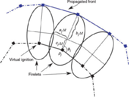
The Huygens’ expansion approach considers every point in the fire front as a virtual ignition point that will expand following an elliptical geometry called a firelet. The curve that envelops all firelets is then the expanded perimeter. The lateral ( ) and the front velocity (
 ) of each firelet (Fig. 3) can be derived from geometrical relationships given RoS and the length-to-breadth ratio
  of the firelet as:
|
 is the wind–slope direction and the subscript j identifies a node of a given fire front.
where  is a front discretisation parameter and
  is the spreading time.
Note that Eqns 5 and 6 satisfy Eqn 7, as this is the distance between the virtual ignition point on the perimeter and its perpendicular expansion as illustrated in Fig. 3.

To determine the length-to-breadth ratio  , we used Anderson’s experimental correlation (Anderson 1983):

where U is the mid-flame wind speed (in m s–1).
The curve enveloping the firelets is calculated using the partial differential equations derived by Richards (1990, 1993) (Eqns 9 and 10), which are resolved using a predictor–corrector method.
where  is the simulation time, and
  is the slope–wind direction, which corresponds to the direction in which the wind is blowing (i.e. where it is blowing towards) if the terrain is flat. Variables x and y are the coordinates of the nodes that constitute a front
  at a given time.
In the present implementation, the mid-flame wind speed  in Eqn 8 and direction
  used in Eqns 9 and 10 are also considered invariants to be identified and are named
  and
and  respectively.
With Eqns 4–10, the final forward model  that provides the output of the set of front perimeters
  for a given simulation time
  can be defined as a function of the initial observed perimeter
  , the fuel depth
  and the invariants vector
  as:
as:


Owing to the Lagrangian formulation of the forward model in hand, when the front exhibits convex regions the Huygens expansion approach may create some loops or overlaps along the perimeter (Fig. 4). These topological problems are physically meaningless and a loop-clipping filter is required to remove these loops and reclose the remaining front. There are different methods in the literature to tackle this problem. The turning number approach (Barber et al. 2008) can be used to identify the front sections that are internal to the curve and filter them out. However, if small integration steps are used in Eqns 9 and 10, the loops do not interact with the perimeter (see left loop in Fig. 4) but just fold in on themselves (right loop depicted in Fig. 4). In this case, the loops can be filtered out by finding the adjacency matrix corresponding to the nodes pj (see Fig. 4) and removing all closed paths.
|
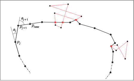
 is the new node introduced by applying the regridding algorithm as
  is larger than the threshold T. (For colour reproduction of figures, see online version available at
 The Lagrangian formulation also yields another problem. As the fire front grows and spreads, the distance between nodes increases and more nodes are needed to avoid formation of sharp unreliable regions (see Fig. 5). This regridding process is conducted by comparing the adjacent angles αj and αj+1 (see Fig. 4) of two consecutive segments of the front. If the largest angle exceeds a given threshold T, an extra node is added at the midpoint of the corresponding segment. With this filter, more nodes are automatically generated in the more abrupt and sharp areas, smoothing the forthcoming simulated isochrones.

|
 . The marker line (red crosses) is the initial fire perimeter. (For colour reproduction of figures, see online version available at
 Optimisation scheme
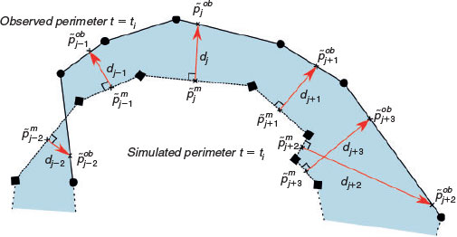
To perform a proper assimilation process, we need to define a cost function ( ) to minimise differences between the observed front and the simulated front. We define this cost function as the sum over all simulated isochrones of the averaged Euclidean distance between simulated and observed fronts. These distances are computed by selecting the modelled (m) points (
 ) in between simulated nodes (
 ) and each point in the corresponding observed (ob) nodes (
 ) determined by perpendicular intersection (as depicted in Fig. 6).
|
Then, the cost function ( ) can be written in terms of the invariants vector
  as:
as:
where  is the number of nodes in each isochrone, the subscript i is the identifier of the simulated (and assimilated) front at any given time, and
  is the weight matrix, which can be set to give more weight to the perimeters assimilated later in time, and give less importance to those assimilated a longer time ago. Note that to efficiently apply the optimisation condition (
 ) of Eqn 13, we take the square of the Euclidian distance (removing the squared root) as it does not affect the optimisation.
For the examples presented in the present study, the identity matrix is used, which represents a homogeneous weight function distribution.
Once the cost function is defined, the inverse problem to find  can be formulated as the following optimisation problem:
for a given initial front with observed coordinates  , fuel depth
  and assimilating period t. The invariants
  cover a range of values that have a physical meaning, with
  and
and  as the maximum invariant values for a given scenario. This turns the optimisation problem into a constrained problem and allows particular optimisation techniques. In the present implementation, if any invariant exceeds these ranges during an assimilation loop, its value is reset to the previous estimated value.
The vector-based cost function definition  is critical because it will drive the invariant’s convergence to the final optimised value. The actual vector-based method used to quantify the dissimilarity between two curves may entail some converging discrepancy when compared with the actual area between curves (see Fig. 6), as some close curves may give large vectored distances – i.e. large values of
  – due to the perpendicular definition even though the area difference is kept small (see Fig. 6). This effect can appear when handling large time steps and irregular front shapes (normally caused by highly heterogeneous terrain or fuel distribution). Thus, although we need a point-to-point function to apply our optimising strategy, we evaluate the area between curves at each optimisation loop to control both convergences.
Two main approaches can be used to solve optimisation problems (Onwubolu and Babu 2013): the gradient-free and the gradient-based algorithms. The former involves searching the optimisation domain to find a global minimum, but is computationally expensive if multiple invariants are used, because the cost function needs to be evaluated multiple times for each invariant change and so does the forward model. On the other hand, the gradient-based strategies do not guarantee an absolute minimum; however, if the forward model behaves smoothly and the algorithm is initialised in the vicinity of the solution, they will provide the correct answer with great computational efficiency (Nocedal and Wright 1999).
Which is the more suitable strategy depends on the particularity of the system and its requirements. The problem at hand is a constrained non-linear optimisation that may have to be solved multiple times during an operational event, and thus has to be computationally efficient. Moreover, we want the algorithm to be ready to handle a larger number of invariants. Therefore, we choose a gradient-based approach.
To speed up the optimisation process, we take advantage of a Tangent Linear Model (TLM) to iteratively linearise the forward model  on the vicinity of a set of parameters (
 ). The TLM is applied by means of a first-order Taylor expansion around an initial parameter estimation
  . The
. The  vector with the initialisation of the invariant values is chosen by an educated guess based on available data.
The gradient of the linearised cost function is then written as:
which can be rewritten as:
which is a linear system that can be rapidly solved for ( ) by using a QR factorisation algorithm (Nocedal and Wright 1999).
To solve the gradient  , we use automatic differentiation (Bischof et al. 2006) because it does not require running the forward model multiple times as more common methods such us central differences (Griewank 2000) do. Adimat software (Bischof et al. 2002) was used to differentiate the code.
Infrared monitoring of real fire behaviour: the Ngarkat experiments
The algorithm was tested with data from two large-scale experimental fires performed in South Australia in March 2008. Despite these being within the framework of a scientific experimental burning program, the fires exhibited real wildfire behaviour patterns as they were performed in large plots under extremely severe weather conditions. These experiments were conducted in Ngarkat Conservation Park (35°45′S, 140°51′E), which consists of a characteristic dune and swale system comprising large flat areas (130 m above sea level) of mallee-heath shrublands. Fire behaviour in mallee-heath fuel types is characterised as being discontinuous and highly variable owing to the heterogeneous characteristics of the various fuel layers that comprise mallee-heath fuel complexes (Cruz et al. 2013).
Data used in the present paper come from two experimental burns. These burns were performed in two different sites named hereafter ‘Shrub site’ and ‘Woodland site’ (plots A and AS2E respectively according to Cruz et al. 2013). The burn in the Shrub site was performed in a 9-ha, 9 year-old heath plot on 4 March 2008. This fuel complex was characterised by scattered small-leafed shrubs, organised in clumps, and a discontinuous litter layer partially buried by sand. The main fire-carrying fuel layer was the discontinuous shrub canopy. Ambient conditions were a temperature of 32°C and relative humidity of 25%. Wind speed (10-m open) averaged 15 km h–1, with gusts up to 30 km h–1. Wind direction was south–south-westerly. The characteristic dead fuel moisture of the fuel complex was 7.7%. The fire was ignited with a 150-m long line and 2 min after ignition, flame heights were ~2–2.5 m, with flashes up to 4 m. The fire spread vigorously throughout the plot with sustained flames heights of 4–5 m. Eight minutes after ignition, the main flame front hit the northern border of the plot, concluding a 350-m head fire run (Planas et al. 2011).
The burn in the Woodland site was performed on 5 March 2008, in a 25-ha plot of a 22-year-old woodland dominated by mallee eucalypts. The fuel complex in this plot was characterised by a mallee overstorey 2 to 3 m tall and a shrubby understorey that constituted the main fuel layer supporting fire propagation. Air temperature was 36°C and relative humidity 13%. The 10-m open wind speed averaged 17 km h–1, gusting up to 36 km h–1. Sampled dead fuel moisture of dead suspended fuels was 7%. The fire was ignited using a 250-m line and initially spread in heath vegetation with flame heights averaging 4 m. As the fire burnt into mallee vegetation, crowning ensued, with flame heights averaging 4.5 m, and peaking at 10 m. A short lull in wind speed 5 min after ignition slowed fire propagation and revealed multiple spot fires along the fire perimeter. As wind speed increased again, the fire made an intense crown fire run in the mallee vegetation, with flame heights between 8 and 10 m and spot fires developing 40–60 m ahead of the fire.
The Woodland site was used to study and characterise aerial suppression efficiency (Plucinski and Pastor 2013). Thus, for the evaluation of the algorithm developed in the present work, only those perimeters before the first aerial drop were used.
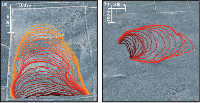
Both plots were filmed from a hovering helicopter equipped with an IR camera. This camera operated within the 7.5–13-µm range and stored sequences of IR images (240 × 320-pixel) at an approximate rate of 5 frames s–1. The helicopter was positioned so that the majority of the plot was in view for the duration of each fire. The images were georeferenced using beacons deployed along the plot as referencing markers and georectified assuming a flat terrain (see Fig. 7). Fire front positions were extracted every 10 s to create isochrones and RoS maps for both plots by applying a methodology for IR analysis described elsewhere (Pérez et al. 2011).

|
The fire in the Shrub site lasted 370 s, giving 38 perimeters at 10-s frequency, although the initial 130 s are considered to be within the artificial linear ignition and were discarded, leaving 25 perimeters available for the current algorithm validation (left plot in Fig. 8). The fire in the Woodland site lasted 450 s but the first drop discharge took place 240 s after ignition. Thus, taking the perimeters from 60 s on to avoid the effect of the artificial ignition, 19 perimeters at 10-s frequency were left for the purpose of the current study (right plot Fig. 8).
|
Results and discussion
The two presented plots are chosen to illustrate the algorithm performance when tested with real data. The wind speed and direction invariants are initialised using approximate values registered during the experiment (simulating the manner the system could be used in a real operation). The  invariant initial value (Table 1) is calculated with Eqns 1 and 2. Required parameters are taken from the standard fire behaviour fuel model SH5 (Scott and Burgan 2005) corresponding to ‘Very high load, dry climate shrubs’ and complemented with values of moisture measured during the Ngarkat experiments (Table 1). The moisture content was measured using the oven-dry method. The upper limits for the invariants
  and
and  are an upper bound needed to set the optimisation problem. Their values were set considering conservative maximum reasonable values for the scenario. In the present examples, those values were never reached.
|
The fuel depth  is considered homogeneous. The system is tested using this approximation as in a real-case scenario where an accurate fuel map might not be available. In the following sections, different outputs of the system are separately evaluated.
Assimilation step
The first factor to validate the system at hand is the assimilation stage. Only if the optimisation algorithm manages to find the proper invariants that model the observed fronts will it be possible to launch a reliable forecast. The assimilating process is iterative and stops when the percentage difference of the invariants between two consecutives loops (named relative error,  ) reaches a threshold of 0.05% as:
where the index k represents each invariant, the superscript i each loop iteration, and  is the invariant initialisation value.
As mentioned before, the area between the curves is tracked to check the correctness of the cost function. The absolute areal error is calculated by summing all the enclosing areas between the simulated front,  , and the corresponding observed front,
  :
:
where  is the XOR logical operator,
  is the absolute areal error and the subscript i corresponds to a given assimilating time.
The match between simulated and observed fronts is evaluated by three similarity indices:
1. SDI′ is the inverted shape deviation index (SDI) (Cui and Perera 2010):
2. Sørensen (Sørensen 1948):
3. Jaccard (Jaccard 1901):
The three similarity indices have a score range of [0–1], 1 being the best score, indicating identical shapes. Their main difference is the denominator identification or, in other words, the normalising factor. Because it is not clear which of the mentioned indexes performs best to quantify simulation correctness (Filippi et al. 2014b), we analyse the three of them.
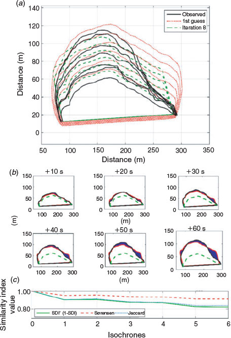
Fig. 9 shows six assimilated isochrones for the Woodland site. The isochrone captured at 40 s after the ignition is used as the initial perimeter  . The subsequent assimilated isochrones span 10 s. The optimisation loop converges after three iterations and the similarity indices are kept over 0.9, showing great resemblance.
|
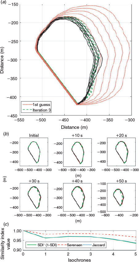
The same procedure is applied to the Shrub site; in this case, six isochrones spanning 10 s are assimilated. The first isochrone corresponds to 140 s after fire ignition. The optimisation loop converges after eight iterations (Fig. 10). The similarity indices are over 0.9 for the three initial fronts and decrease to 0.8 owing to imperfect simulation of the right flank. This flank showed an extremely low RoS that could not be fully replicated by the forward model as only one common lateral RoS ( ) is resolved.
|
In both cases, the assimilation stage shows great ability to model the front data regardless of the number of assimilated isochrones.
Invariants convergence
The effectiveness of the algorithm relies on the individual convergence of each invariant. Only if they are all individually resolved will their value be meaningful and useful to run the forecast. For each assimilation, the convergence of the cost function and the invariants’ individual convergence is tracked and displayed in Fig. 11 and Fig. 12.

|

|
 invariant fluctuation is due to the nature of angular direction restricted to [0–2π].
The invariant relative error ( , Eqn 17) shows how far from the final value the invariant was initialised. For the Woodland site, the invariants converge to values of 0.542 s–1, 2.651 m s–1 and 0.569 rad (see Table 1), which represents a change from the initial values of 500%, –80% and 25% (Fig. 11). Applying Eqn 3 and assuming an average fuel depth of 1.4 m, the
  invariant can be expressed as a RoS with the value of 45.5 m min–1. This value represents a RoS average for the whole perimeter during the assimilation period and is in agreement with the values reported in Planas et al. (2011) where RoS was found to range between 20 and 60 m min–1 along the whole perimeter. The wind speed and direction also had reasonable values although more detailed data are not available for comparison.
The vector cost function calculated as Eqn 13 converges to 1.2 m (see Fig. 11), which indicates the average normal distance between simulated and observed fronts. At the same time, the sum of the absolute areal error for all perimeters converges to a value of 1363 m2.
Similar results are obtained for the Shrub site (see Fig. 12). In this case, invariants converge to the values 0.447 s–1, 5 m s–1 and 5.95 rad, which represent an average RoS of 10.4 m min–1. The values observed in Planas et al. (2011) ranged from 5 to 40 m min–1. In this case, the average distance between simulated and observed fronts is ~4 m whereas the areal distance is 2135 m2. As mentioned before, both convergence indicators do not follow exactly the same behaviour and the vector-based one finds a minimum before stabilising. This highlights the need for an areal-based cost function instead of a vector-based one.
Forecasting step
Once the invariants are resolved, we can launch a forecast using the last assimilated isochrone as the initial perimeter ( ) and propagate it with the forward model while assessing its efficiency. For each case explored, the observed available fronts are split into two groups. The first is used as data assimilation input whereas the second group is reserved for evaluating the correctness of the forecast. In addition to the forecasting error, to evaluate the appropriateness of the system, the lead time must be computed. The lead time is defined as the period of validity of the model once the computational time is subtracted. In order for the model to be operative, the lead time needs to be positive. For the current exploration, we considered the forecast to be valid as long as the SDI′ index was kept over 0.85.
Following the already defined scenarios, when five isochrones are assimilated every 10 s in the Woodland site, the lead time reaches 130 s as the similarity index gradually decreases, reaching the 0.85 threshold (see Fig. 13). The forecast run for the Shrub site, when six fronts are assimilated, yields a larger lead time. Although the similarity indices decrease to 0.8 at 50 s, they stabilise at 0.9 for the rest of the available fronts, as shown in Fig. 14.

|

|
From this point on, the fire behaviour in the right flank changes, accelerating the rate of spread, and the forecasted front is therefore underpredicted. The underlying cause might be due to the fact that Rothermel’s model was initially derived for surface fire spread. As fire propagates through crowns, the model is no longer valid, although a proper assimilation structure extends its validity as fire in the Woodland site was erratically torching and crowning.
It is important to mention that the forecasting step can be improved by adding extra layers of information, particularly those that can change in time and space (i.e. fuels depth map, wind speed and direction, etc.). If those layers are available, the lead time can be improved as the present algorithm cannot resolve time-dependent variables.
Assimilation window exploration
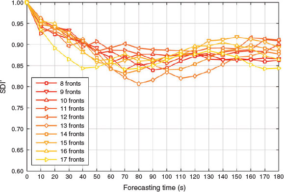
If the algorithm is to be used operationally, the consequences of the amount and frequency of assimilated data need to be investigated. The assimilation window (AW) is defined as the number of fronts assimilated before launching a forecast. To explore this, we use the Shrub site to run our assimilation and forecasting system 12 times, changing the number of assimilated fronts. The assimilation window varies from 8 assimilated fronts (i.e. 70 s) up to 19 assimilated fronts (i.e. 180 s) in the last run. The last assimilated front is kept constant for all runs and corresponds to 190 s after ignition. Then, the forecast is launched to generate the 18 fronts corresponding to the 180 s left of observed data. The areal relative error is computed to assess the validity of each forecast.
The results are shown in Fig. 15. As more fronts are assimilated, the SDI′ index tends to stabilise at ~0.87. It is interesting to note that, for the current experiment, there is an optimum AW at ~11–12 assimilated fronts where the lead time is maximised and reaches 180 s. As more than 12 fronts are assimilated, the fronts corresponding to times close to ignition are taken into account. In particular, when 17 fronts are assimilated, the first assimilated isochrone corresponds to 10 s after the ignition. At this stage, the fire is still driven by initial acceleration effects, and thus the forecast slightly overestimates the RoS and the forecasting areal error tends to grow, dramatically decreasing the lead time.
|
Concluding remarks
We present a data assimilation framework that enhances a Rothermel-based model to make it capable of forecasting short-term wildfire dynamics even when using it beyond its original applicability scenarios. The assimilation framework previously applied to synthetically generated data is improved to deal with real scenarios and tested in two large-scale shrubland fire experiments conducted in South Australia, yielding similarity index scores over 0.8 and obtaining positive lead times of 130 and 160 s, depending on the scenario. The system performance when changing the AW is explored to conclude that the more fronts are assimilated, the better the forecast validity, up to a point where the initial fire dynamics perturb the forecast. Different forms of the weighting matrix present in the cost function are also explored in depth although improvement is limited.
Even though in the present work the available fire data last a few minutes and extend up to several hundred metres, the algorithm structure is envisaged to be applied at larger time and space scales. At the operational level, the time required to perform image processing tasks such as georeferencing and fire front edge detection must be considered as they will directly affect the lead time. Current work is being done to automate and improve those tasks (Valero et al. 2015).
In the future, the algorithm will be prepared to handle non-flat terrain scenarios by interacting with digital terrain models input beforehand. Time-varying inputs (such as wind speed or moisture content) will be used to enlarge the lead time and take full advantage of the available data. Space-dependent invariants will be explored to handle fuel and fire dynamics heterogeneity. Finally, the algorithm will be implemented recursively as we believe that by running it systematically, the fire spread prediction could be updated and extended to provide a sound operational tool.
| List of symbols, quantities and units used in equations and text |
| Variables |
|
| Indices |
|
 Lateral firelet propagation velocity (m s–1)
 Two-node adjacent angle (rad)
 Firelet partial front velocity, starting at the centre of the firelet (m s–1)
 Fuel packing ratio (–)
 Firelet partial front velocity, starting at the ignition point (m s–1)
 Euclidian distance (m)
 Fuel depth (m)
 Effective heating factor (–)
 Relative error (%)
 Absolute areal error (m2)
 Propagating flux ratio (–)
 Rothermel’s slope factor (–)
 Rothermel’s wind factor (–)
 Reaction intensity (J m–2 s–1)
 Wind speed invariant (m s–1)
 Wind direction invariant (rad)
 Fuel–wind invariant (1 s–1)
 Cost function
 Firelet length-to-breadth ratio (–)
 Forward model
 Moisture content (%)
 Moisture of extinction (%)
 Number of isochrones
 Number of front nodes
 Principal fire front node
 Auxiliary fire front node
 Heat of preignition (J kg–1)
 Invariants vector
 Bulk density (kg m–3)
 Front discretisation parameter (–)
 Regridding angular threshold
 Simulation time (s)
 Mid-flame wind speed (m s–1)
 Weighting matrix
 Oven-dried fuel loading (kg m–2)
 Set of front coordinates
 Slope–wind direction (rad)
 Final
Final Isochrones index
 Node index
 Iteration index
 Simulated
 Maximum value
 Observed
 Initial
Acknowledgements
The authors are grateful to the Spanish Ministry of Economy and Competitiveness (project CTM2014–57448-R), the Spanish Ministry of Education, Culture and Sport (Formación de Profesorado Universitario Program) and the Autonomous Government of Catalonia (project no. 2014-SGR-413). The authors also thank Guillermo Rein for initial ideas and insights into inverse modelling. The South Australia experiments were funded by the Bushfire Cooperative Research Centre, CSIRO Ecosystem Sciences and CSIRO Climate Adaptation Flagship.
References
Anderson HE (1983) Predicting wind-driven wildland fire size and shape. USDA Forest Service, Intermountain Forest and Range Experiment Station, Research Paper INT-305. (Ogden, UT)Artés T, Cencerrado A, Cortés A, Margalef T, Rodríguez-Aseretto D, Petroliagkis T, San-Miguel-Ayanz J (2014) Towards a dynamic data-driven wildfire behavior prediction system at European level. Procedia Computer Science 29, 1216–1226.
| Towards a dynamic data-driven wildfire behavior prediction system at European level.Crossref | GoogleScholarGoogle Scholar |
Barber J, Bose C, Bourlioux A (2008) Burning issues with PROMETHEUS – the Canadian wildland fire growth simulation model. Canadian Applied Mathematics Quarterly 16, 337–378.
Bischof CH, Bücker HM, Lang B, Rasch A, Vehreschild A (2002) Combining source transformation and operator overloading techniques to compute derivatives for MATLAB programs. In ‘Proceedings, Second IEEE international workshop on source code analysis and manipulation (2002)’, 1 October 2002, Montreal, PQ. IEEE Computer Society, pp. 65–72 (Los Alamitos, CA)
Bischof CH, Büucker H, Vehreschild A (2006) A macro language for derivative definition in ADiMat. In ‘Lecture notes in computational science and engineering, Vol. 50’. (Eds M Bücker, G Corliss, P Hovland, U Naumann, B Norris) pp. 181–188. (Springer-Verlag: Berlin)
Bova AS, Mell WE, Chad MH (2016) A comparison of level set and marker methods for the simulation of wildland fire front propagation International Journal of Wildland Fire 25, 229–241.
| A comparison of level set and marker methods for the simulation of wildland fire front propagationCrossref | GoogleScholarGoogle Scholar |
Cruz MG, Alexander ME (2013) Uncertainty associated with model predictions of surface and crown fire rates of spread. Environmental Modelling & Software 47, 16–28.
| Uncertainty associated with model predictions of surface and crown fire rates of spread.Crossref | GoogleScholarGoogle Scholar |
Cruz MG, McCaw W, Anderson WR, Gould JS (2013) Fire behaviour modelling in semi-arid mallee-heath shrublands of southern Australia. Environmental Modelling & Software 40, 21–34.
| Fire behaviour modelling in semi-arid mallee-heath shrublands of southern Australia.Crossref | GoogleScholarGoogle Scholar |
Cui W, Perera AH (2010) Quantifying spatiotemporal errors in forest fire spread modelling explicitly. Journal of Environmental Informatics 16, 19–26.
| Quantifying spatiotemporal errors in forest fire spread modelling explicitly.Crossref | GoogleScholarGoogle Scholar |
Denham M, Wendt K, Bianchini G, Cortés A, Margalef T (2012) Dynamic data-driven genetic algorithm for forest fire spread prediction. Journal of Computational Science 3, 398–404.
| Dynamic data-driven genetic algorithm for forest fire spread prediction.Crossref | GoogleScholarGoogle Scholar |
Filippi JB, Bosseur F, Mari C, Lac C, Le Moigne P, Cuenot B, Veynante D, Cariolle D, Balbi J-H (2009) Coupled atmosphere–wildland fire modelling. Journal of Advances in Modeling Earth Systems 1, 11
| Coupled atmosphere–wildland fire modelling.Crossref | GoogleScholarGoogle Scholar |
Filippi JB, Bosseur F, Grandi D (2014a) ForeFire: open-source code for wildland fire spread models. In ‘Advances in forest fire research’. (Ed. DX Viegas) (Imprensa da Universidade de Coimbra: Coimbra, Portugal)
Filippi JB, Mallet V, Nader B (2014b) Evaluation of forest fire models on a large observation database. Natural Hazards and Earth System Sciences 14, 3077–3091.
| Evaluation of forest fire models on a large observation database.Crossref | GoogleScholarGoogle Scholar |
Filippi JB, Mallet V, Nader B (2014c) Representation and evaluation of wildfire propagation simulations. International Journal of Wildland Fire 23, 46–57.
| Representation and evaluation of wildfire propagation simulations.Crossref | GoogleScholarGoogle Scholar |
Finney M (1998) FARSITE: FireArea Simulator – model development and evaluation. USDA Forest Service, Rocky Mountain Research Station, Research Paper RMRS-RP-4. (Fort Collins, CO)
Finney M, Cohen JD, McAllister SS, Jolly WM (2013) On the need for a theory of wildland fire spread. International Journal of Wildland Fire 22, 25–36.
| On the need for a theory of wildland fire spread.Crossref | GoogleScholarGoogle Scholar |
Glasa J, Halada L (2008) On elliptical model for forest fire spread modeling and simulation. Mathematics and Computers in Simulation 78, 76–88.
| On elliptical model for forest fire spread modeling and simulation.Crossref | GoogleScholarGoogle Scholar |
Griewank A (2000) ‘Evaluating derivatives: principles and techniques of algorithmic differentiation.’ (SIAM: Philadelphia, PA)
Jaccard P (1901) Étude comparative de la distribution florale dans une portion des Alpes et du Jura. Bulletin de la Société Vaudoise des Sciences Naturelles 37, 547–579.
Lautenberger C (2013) Wildland fire modeling with an Eulerian level set method and automated calibration. Fire Safety Journal 62, 289–298.
| Wildland fire modeling with an Eulerian level set method and automated calibration.Crossref | GoogleScholarGoogle Scholar |
Linn R (1997) A transport model for prediction of wildfire behavior. Los Alamos National Laboratory, Science Report LA-13334-T. (Los Alamos, NM)
Mallet V, Keyes DE, Fendell FE (2009) Modeling wildland fire propagation with level set methods. Computers & Mathematics with Applications 57, 1089–1101.
| Modeling wildland fire propagation with level set methods.Crossref | GoogleScholarGoogle Scholar |
Mandel J, Beezley JD, Coen JL, Kim M (2009) Data assimilation for wildland fires. IEEE Control Systems 29, 47–65.
| Data assimilation for wildland fires.Crossref | GoogleScholarGoogle Scholar |
Mandel J, Beezley JD, Kochanski K (2011) Coupled atmosphere–wildland fire modeling with WRF 3.3 and SFIRE 2011. Geoscientific Model Development 4, 591–610.
| Coupled atmosphere–wildland fire modeling with WRF 3.3 and SFIRE 2011.Crossref | GoogleScholarGoogle Scholar |
Mandel J, Amram S, Beezley JD, Kelman G, Kochanski AK, Kondratenko VY, Lynn BH, Regev B, Vejmelka M (2014) Recent advances and applications of WRF-SFIRE. Natural Hazards and Earth System Sciences 14, 2829–2845.
| Recent advances and applications of WRF-SFIRE.Crossref | GoogleScholarGoogle Scholar |
Mell W, Jenkins M, Gould J, Cheney P (2007) A physics-based approach to modelling grassland fires. International Journal of Wildland Fire 16, 1–22.
| A physics-based approach to modelling grassland fires.Crossref | GoogleScholarGoogle Scholar |
Nocedal J, Wright SJ (Eds) (1999) ‘Numerical optimization.’ (Springer-Verlag: New York)
Onwubolu GC, Babu BV (2013) ‘New optimization techniques in engineering.’ (Springer-Verlag: Berlin)
Pérez Y, Pastor E, Planas E, Plucinski M, Gould J (2011) Computing forest fires aerial suppression effectiveness by IR monitoring. Fire Safety Journal 46, 2–8.
| Computing forest fires aerial suppression effectiveness by IR monitoring.Crossref | GoogleScholarGoogle Scholar |
Perry GLW, Sparrow AD, Owens IF (1999) A GIS-supported model for the simulation of the spatial structure of wildland fire, Cass Basin, New Zealand. Journal of Applied Ecology 36, 502–518.
| A GIS-supported model for the simulation of the spatial structure of wildland fire, Cass Basin, New Zealand.Crossref | GoogleScholarGoogle Scholar |
Planas E, Pastor E, Cubells M, Cruz MG, Greenfell I (2011) Fire behaviour variability in mallee-heath shrubland fires. In ‘5th International Wildland Fire Conference’, 9–13 May 2011, Sun City, South Africa.
Plucinski M, Pastor E (2013) Criteria and methodology for evaluating aerial wildfire suppression. International Journal of Wildland Fire 22, 1144–1154.
| Criteria and methodology for evaluating aerial wildfire suppression.Crossref | GoogleScholarGoogle Scholar |
Richards G (1990) An elliptical growth model of forest fire fronts and its numerical solution. International Journal for Numerical Methods in Engineering 30, 1163–1179.
| An elliptical growth model of forest fire fronts and its numerical solution.Crossref | GoogleScholarGoogle Scholar |
Richards GD (1993) The properties of elliptical wildfire growth for time-dependent fuel and meteorological conditions. Combustion Science and Technology 95, 357–383.
| The properties of elliptical wildfire growth for time-dependent fuel and meteorological conditions.Crossref | GoogleScholarGoogle Scholar |
Rios O, Jahn W, Rein G (2014) Forecasting wind-driven wildfires using an inverse modelling approach. Natural Hazards and Earth System Sciences 14, 1491–1503.
| Forecasting wind-driven wildfires using an inverse modelling approach.Crossref | GoogleScholarGoogle Scholar |
Rochoux M, Emery C, Ricci S, Cuenot B, Trouvé A (2014a) Towards predictive simulation of wildfire spread at regional scale using ensemble-based data assimilation to correct the fire front position. Fire Safety Science 11, 1442–1456.
| Towards predictive simulation of wildfire spread at regional scale using ensemble-based data assimilation to correct the fire front position.Crossref | GoogleScholarGoogle Scholar |
Rochoux M, Ricci S, Lucor D, Cuenot B, Trouvé A (2014b) Towards predictive data-driven simulations of wildfire spread – Part I: Reduced-cost ensemble Kalman filter based on a polynomial chaos surrogate model for parameter estimation. Natural Hazards and Earth System Sciences 14, 2951–2973.
| Towards predictive data-driven simulations of wildfire spread – Part I: Reduced-cost ensemble Kalman filter based on a polynomial chaos surrogate model for parameter estimation.Crossref | GoogleScholarGoogle Scholar |
Rochoux M, Emery C, Ricci S, Cuenot B, Trouvé A (2015) Towards predictive data-driven simulations of wildfire spread – Part II: Ensemble Kalman filter for the state estimation of a front-tracking simulator of wildfire spread. Natural Hazards and Earth System Sciences 15, 1721–1739.
| Towards predictive data-driven simulations of wildfire spread – Part II: Ensemble Kalman filter for the state estimation of a front-tracking simulator of wildfire spread.Crossref | GoogleScholarGoogle Scholar |
Rothermel RC (1972) A mathematical model for predicting fire spread in wildland fuels. USDA Forest Service, Intermountain Forest and Range Experiment Station, Research Paper INT-RP-115. (Ogden, UT)
Scott JH, Burgan RE (2005) Standard fire behavior fuel models: a comprehensive set for use with Rothermel’s surface fire spread model. Available at http://www.fs.fed.us/rm/pubs/rmrs_gtr153.pdf [Verified 14 July 2016]
Sørensen T (1948) A method of establishing groups of equal amplitude in plant sociology based on similarity of species and its application to analyses of the vegetation on Danish commons, Biologiske Skrifter 5, 1–34.
Sullivan AL (2009) Wildland surface fire spread modelling, 1990–2007. 1: Physical and quasi-physical models. International Journal of Wildland Fire 18, 349–368.
| Wildland surface fire spread modelling, 1990–2007. 1: Physical and quasi-physical models.Crossref | GoogleScholarGoogle Scholar |
Tolhurst K, Shields B, Chong D (2008) Phoenix: development and application of a bushfire risk management tool. Australian Journal of Emergency Management 23, 47–54.
Tymstra C, Bryce R, Wotton B (2010) ‘Development and structure of Prometheus: the Canadian wildland fire growth simulation model.’ (Northern Forestry Centre: Edmonton, AB)
Valero MM, Rios O, Pastor E, Planas E (2015) Automatic detection of wildfire active fronts from aerial thermal infrared images. In ‘13th International Workshop on Advanced Infrared Technology and Applications: Proceedings’, 29 September–2 October, Pisa, Italy. pp. 63–67.
Viegas DX (2011) Overview of forest fire propagation research. Fire Safety Science 10, 95–108.
| Overview of forest fire propagation research.Crossref | GoogleScholarGoogle Scholar |
Wendt K, Denham M, Cortés A, Margalef T (2011) Evolutionary optimisation techniques to estimate input parameters in environmental emergency modelling. Studies in Computational Intelligence 359, 125–143.
| Evolutionary optimisation techniques to estimate input parameters in environmental emergency modelling.Crossref | GoogleScholarGoogle Scholar |