

Quantification of secondary organic aerosol in an Australian urban location
Melita Keywood A D , Helen Guyes B C , Paul Selleck A and Rob Gillett AA Centre for Australian Weather and Climate Research and CSIRO Marine and Atmospheric Research, PMB1, Aspendale, VIC 3195, Australia.
B School of Mathematical Sciences, Monash University, VIC 3800, Australia.
C Present address: Department of Climate Change and Energy Efficiency, GPO Box 854, Canberra, ACT 2601, Australia.
D Corresponding author. Email: melita.keywood@csiro.au
Environmental Chemistry 8(2) 115-126 https://doi.org/10.1071/EN10100
Submitted: 6 September 2010 Accepted: 3 December 2010 Published: 2 May 2011
Journal Compilation © CSIRO Publishing 2011 Open Access CC BY-NC-ND
Environmental context. Particulate matter is detrimental to human health necessitating air quality standards to ensure that populations are not exposed to harmful levels of air pollutants. We quantified, for the first time in an Australian city, secondary organic aerosol produced in the atmosphere by chemical reactions, and show that it constitutes a significant fraction of the fine particulate matter. Secondary organic aerosol should be considered in regulations to control particulate matter and ozone.
Abstract. The contribution of secondary organic aerosol (SOA) to particulate mass (PM) in an Australian urban airshed is quantified for the first time in this work. SOA is estimated indirectly using the elemental carbon tracer method. The contribution of primary organic carbon (OC) to PM is determined using ambient air quality data, which is used to indicate photochemical activity and as a tracer for a general vehicular combustion source. In addition, levoglucosan concentrations were used to determine the contribution of wood heater emissions to primary OC. The contribution of bushfire smoke to primary OC emissions was determined from the organic and elemental carbon (OC/EC) ratios measured in bushfire source samples. The median annual SOA concentration determined in this work was 1.1 µg m–3, representing ~13% of PM2.5 median concentrations on an annual basis (assuming a ratio of organic mass (OM) to OC of 1.6). Significantly higher SOA concentrations were determined when bushfire smoke affected the airshed; however, the SOA fraction of PM2.5 was greatest during the autumn and early winter months when the formation of inversions allows build up of particles produced by domestic wood-heater emissions.
Additional keywords: EC tracer method, primary carbon.
Introduction
Urban aerosol is a complex mixture of primary and secondary compounds, where primary compounds are emitted directly to the atmosphere from sources such as industrial activity, transportation, power generation and natural processes (e.g. wind blown dust, oceanic bubble bursting and volcanic eruptions) and secondary compounds result from gas to particle conversion and heterogeneous reactions within the atmosphere. Carbonaceous material has been found to comprise a significant fraction (20–90%) of fine particulate matter (PM2.5) in urban areas and comprises two fractions, organic carbon (OC) and elemental carbon (EC).[1–3] EC is a primary pollutant introduced into the atmosphere by combustion, whereas OC is a complex mixture of many groups of compounds that are derived from both primary sources and secondary formation processes.[4] These characteristics of OC and EC form the basis for the determination of secondary organic aerosol (SOA) using the OC/EC method originally devised by Turpin and Huntzicker[1] and subsequently refined by others.[2,5,6]
SOA is produced in the atmosphere by the oxidation of volatile organic compounds (VOCs) of biogenic or anthropogenic origin, to produce semi-volatile compounds that may partition to existing particles. A great deal of uncertainty exists around the process of SOA formation, which is unsurprising if we consider that the number of VOCs that have been measured in the atmosphere is estimated to be 10 000 to 100 000[7] and that each VOC can undergo several different reactions to produce a range of oxidised products that may or may not result in SOA formation.
Until this work, the only estimates of the contribution of SOA to particulate mass (PM) in Australian cities were those carried out by Gras et al.[8] and Gras[9] where SOA was grouped with secondary inorganic aerosol as secondary aerosol. However, the presence of SOA in Australian cities can be predicted as VOCs and oxidants such as sunlight, O3 and oxides of nitrogen and sulfur are all present in Australian cities. The extent of the SOA contribution to PM in Australian cities may affect compliance to air quality standards and regulation to reduce primary aerosol and ozone may in turn affect SOA formation. For example, Docherty et al.[10] suggest that greater ratios of SOA to primary organic aerosol (POA) measured than previously reported during the Los Angeles Study of Organic Aerosols in Riverside (SOAR-1) may indicate an increase in SOA over time resulting from more efficient POA emissions reduction (due to targeted policies such as vehicle emission controls), than reduction of SOA precursors. In addition, recent epidemiological research suggests that human morbidity and mortality may be related to the fine fraction of PM (PM2.5)[11]; however, the mechanism for this relationship is still not understood.
SOA has been quantified in several urban locations, including various cities in North America, Europe and Asia. The contribution of SOA to PM has been found to vary significantly – a few examples are given here. During the Pittsburgh Air Quality Study,[6] 35% of OC was secondary. In Los Angeles during the SOAR-1 measurement campaign in summer 2005, SOA comprised 70–90% of organic aerosol during midday periods and ~45% of organic aerosol during peak traffic periods.[10] In Milan during the summer months (2002 and 2003),[12] SOA comprised 85% of OC (and 35% of PM2.5 or 7 µg m–3). In Zurich secondary aerosols with biogenic sources were responsible for 25% of OC during winter and 48% during summer.[13] Secondary organic carbon (SOC) comprised on average 6.8% of PM2.5 at eight sites in the Pearl River Delta region of China during winter 2001.[14] The highest SOC was observed in Guangzhou, the largest city in Southern China. Duan et al.[15] subsequently confirmed that SOA is a minor component of PM2.5 in Guangzhou during both winter and summer months (4.2–6.8% of PM2.5).
Until the recent development of instrumentation such as the Aerosol Mass Spectrometer, SOA could only be measured indirectly. The most commonly applied method has been the EC tracer method,[1] on which the research presented in this paper is based. The EC tracer method has several limitations (and these will be discussed throughout the paper); however, the method is relatively routine and inexpensive so is well suited for long-term measurement programs. Although technology now exists to make more direct measurements of SOA (e.g. the Aerosol Mass Spectrometer), such technology is not yet suitable for long-term survey studies mainly due to its cost and technical support required. A recent review of emerging issues associated with research into SOA[16] suggests that new methods for the quantification of SOA in the field are still required and that at present the best approach to the problem of SOA quantification is to utilise several different methods in a field campaign to allow for a more complete analysis.
The aim of the present paper is to present the first quantification of SOA to an Australian urban location. SOA is estimated indirectly using a refined version of the EC tracer method.[1] The EC tracer method as a surrogate for SOA determination is based on EC having only a primary source. However, both EC and OC are produced by incomplete combustion so the method relies on understanding the OC/EC ratio contributed by primary sources (OC/ECpri). Ambient aerosol OC/EC ratios greater than OC/ECpri can be attributed to SOA.
Methods to determine OC/ECpri include: (a) using emissions inventory data to calculate the weighted OC/EC for emissions from dominant sources such as motor vehicles and vegetation; (b) examination of ambient OC/EC over a sampling campaign (or single day) where OC/EC data with a probable influence from SOA is neglected; and (c) modelling primary emissions and SOA formation.
In this work we use a combination of methods (a) and (b) to determine OC/ECpri. We use ambient data to determine a general OC/ECpri (OC/ECpr_GEN) that can also be considered OC/ECpri for vehicle emissions (in the absence of other sources), as EC is linked to combustion and the dominant source of PM in the urban environment is from motor vehicle emissions.[17] We also use ambient data to determine an OC/ECpri for wood smoke from wood heaters (OC/ECpri_WH) and source samples of bushfire smoke to determine an OC/ECpri for bushfires (OC/ECpri_BF).
EC can be used to track primary OC, establishing the following relationship between primary and secondary OC:

The primary fraction of OC can be subtracted from the measured OC to give the amount of secondary OC:

Organic mass (OM) is calculated from OC, accounting for the presence of oxygen and hydrogen atoms, by multiplying OC by a factor, that traditionally has been 1.4 (value was based upon speciation data collected over 2 days in Pasadena during the 1970s[18]). However, subsequent studies have suggested 1.4 represents the lower limit of the factor. Turpin and Lim[18] reviewed several organic composition speciated datasets from North America to determine a factor of 1.6 ± 0.2 for urban locations; using the high resolution aerosol mass spectrometry Zhang et al.[19] estimated an average value of 1.8 for submicron Pittsburgh aerosol (a value of 2.2 was measured for the oxygenated fraction of the organic aerosol) and Aitken et al.[20] determined a value of 1.7 for submicron Mexico City aerosol. It is clear that a significant level of uncertainty exists in the value of the factor used to calculate OM from OC, and some of this may lie in the location-dependency of the factor. We note that the factor has not been determined for urban airsheds in Australia. In light of this we adopt the factor of 1.6 and recommend its measurement in future measurement campaigns. Thus the mass of SOA is calculated according to (3):

Results
One hundred thirty-three 24-h PM10 ambient samples spanning 21 months were collected from the Bayside Air Quality Station (BAQS) at Aspendale in Melbourne and their carbon content determined. In addition, the OC/EC ratios of six bushfire samples and four roadway tunnel samples (representative of the average Melbourne vehicle fleet) were used to build profiles of primary sources. The number of samples used to determine the OC/EC ratios for these two sources is similar to those used in other studies as shown in Table 1.

|
Ambient samples
Table 2 lists the minimum, maximum, average and median concentrations of OC, EC and total carbon (TC, where TC is the sum of OC and EC) measured in 133 samples collected at BAQS. The minimum OC/EC ratio (1.62 ± 0.14) occurred in winter on 2 August 2006 and the maximum OC/EC ratio (14.75 ± 0.14) occurred in summer on 1 January 2006 (when smoke from bushfires to the north-east of Melbourne affected the sampling site).
|
Chemical mass (or the sum of total carbon and soluble inorganic ions) made up 70% of PM10 on average over the sampling period. TC comprised up to 66% of the chemical mass.
OC was correlated with select gas, ion and PM2.5 measurement data. The most significant correlation was a linear relationship between OC in the PM10 samples, and TEOM PM2.5 concentrations (R2 = 0.92) suggesting that OC lies within the aerosol fraction less than 2.5 μm. Carbon concentrations are subsequently reported as a percentage of PM2.5.
The time series of measured PM2.5 concentration and the fraction of PM2.5 made up of TC are shown in Fig. 1. The Victorian Alpine Fire Complex of December 2006–January 2007 dominates the aerosol concentration during this period with PM2.5 concentrations reaching 160 μg m–3. A bushfire is also evident during the previous summer in January 2006. There were in fact 11 exceedances of the daily advisory National Environment Protection Measure (NEPM) for PM2.5, between May 2005 and February 2007, five of which were associated with bushfire smoke.
|
Besides the bushfire events, the PM2.5 concentration is raised in late autumn–early winter periods (April–June). Wood heaters are used in Melbourne during both autumn and winter[21] and prescribed burning usually occurs during April. Autumn–early winter in Melbourne is marked by low wind speeds and cool temperatures, thus allowing pollutants to stagnate.[22] Levoglucosan measurements made on PM10 filters collected at BAQS during 2007–09 confirm the presence of smoke in PM10 aerosol during autumn–early winter. Environment Protection Authority Victoria (EPAV) air monitoring reports for 2005 and 2006 ascribe one exceedance of the Air NEPM for PM10 during autumn of both 2005 and 2006 to prescribed burning.[23,24] The remainder of the exceedances the EPAV ascribes to ‘urban’, which is defined as particles accumulating in stable atmospheric conditions, typically from motor vehicles or domestic wood heaters.
The autumn–early winter periods are also marked by high TC/PM2.5 ratios (60–80%) compared with the summer months (20–40%). The TC/PM2.5 ratios from the autumn–early winter periods are also higher than the samples from the bushfire periods (30–50%) collected from December 2006 to January 2007.
The basis of using the OC/EC ratio as a surrogate measurement of SOA is that EC is only emitted from combustion, is therefore primary, and so should be linearly related to primary OC. Any difference between measured OC and primary OC is hence considered secondary OC. In order to demonstrate the relationship between EC and primary OC, previous studies have shown a high degree of correlation between EC and OC in winter months and poor correlation in summer months when secondary processes elevate OC with respect to EC. For example, a correlation of 0.94 for OC and EC was observed in winter PM2.5 samples, compared with a correlation of 0.46 in summer in Madrid.[25] The data from BAQS were similarly analysed for two full winters and one and a half summers to reveal OC, EC correlations of 0.92 and 0.99 respectively. The extraordinarily high summer correlation was due to the summer bushfires and with these events removed, the summer correlation dropped to 0.73. These correlations between OC and EC in BAQS winter and summer values suggest the dominance of primary emissions in winter and a greater occurrence of secondary processes during summer. However, the summertime OC/EC ratio measured in the BAQS data is considerably higher than the ratio measured during summer in Madrid, suggesting the presence of greater amounts of secondary OC in Madrid during summer. This may be owing to the conditions (e.g. temperature, presence of oxidants and precursor species) for secondary OC formation being more favourable in the summertime Madrid atmosphere.
Source samples
The primary OC/EC for the Melbourne road fleet determined from the tunnel samples is presented in Table 1 and consistent with aggregate vehicle exhaust OC/EC reported elsewhere.[12,26] Motor vehicle emissions are the dominant source of air pollution in Melbourne.[8] The OC/EC measured for the tunnel samples is less than 1, suggesting that the samples were heavily influenced by the diesel vehicles using the tunnel.
The OC/EC measured in fresh bushfire smoke samples collected in north-east Victoria ranged between 5.71 and 8.76, with the average shown in Table 1. This value is at the lower end of the range of values reported in the literature, and most close to that measured by Watson and Chow[27] for burning of asparagus farms near the California–Mexico border.
Determination of OC/ECpri for different sources from ambient samples
General OC/ECpri
Fig. 2 shows the relationship between OC and EC for all sample days. Several outlying points with high OC and consequently high OC/EC correspond to two periods (January 2006 and between December 2006 and February 2007) when smoke from the bushfires burning around Melbourne affected Melbourne’s airshed. These data points have been identified in Fig. 2 and removed from the dataset used to determine OC/ECpri as they are clearly not representative of typical Melbourne emissions, and will be discussed later. However, for these days affected by bushfires the OC/ECpri_BF of 7.64 is used based on the measurement of OC/EC in bushfire smoke source samples discussed above.
|
As significant rainfall events remove aged aerosol (that may have a high secondary component) samples with 24-h rainfall amounts greater than 2 mm on the sample day or a day immediately preceding the sample day, are also identified in, and removed from the dataset used to determine OC/ECpri (Fig. 2).
Days with high likelihood of SOA formation were excluded using maximum hourly O3 concentrations for each sample day as an indication of photochemical activity. Maximum hourly O3 concentrations greater than the 90th percentile value (36 ppb) were used to indentify 11 days when significant photochemical activity may have occurred (identified in Fig. 3). The highest maximum hourly O3 concentration was 56 ppb (observed in March 2006).
|
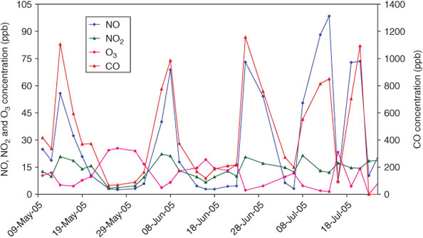
The OC/ECpri was then determined from a subset of ambient measurements following the methodology of Cabada et al.[6] where O3 was used as an indicator of photochemical activity (and hence periods when secondary OC was present) and tracers for combustion sources (NOx, NO and CO) were used to identify periods when primary OC was present. CO and NO were used as indicators of motor vehicle primary emissions, as motor vehicles emit 92% of CO and 86% of NOx in the Melbourne airshed[28] and are a ubiquitous source of primary particles. Fig. 4 shows that peaks concentrations of CO and NO were largely coincident in time. Fifteen days were selected on the basis of high CO and NO (average CO greater than the 80th percentile value) and low maximum hourly O3 (maximum hourly O3 lower than the 30th percentile value). Days with high photochemistry (maximum hourly O3 greater than 30 ppb) were observed at any time of the year, whereas the criteria for primary vehicle events were met only between April and July of each year.
|
For the days dominated by primary motor vehicle emissions identified in Fig. 3 reduced major axis linear regression was applied to obtain the following relationship between OC and EC:

From this relationship, OC/ECpri is 2.248 and a y intercept term, or non-combustion contribution to OC/ECpri is 0.242. We use this value as our OC/ECpri_GEN. These values compare well to those presented elsewhere.[6] However, the OC/ECpri_GEN is greater than the OC/EC measured in the Melbourne tunnel samples (Table 1). There are several possible reasons for this. There was likely a greater incidence of diesel vehicle use in the tunnel, which is a major cross-city transport route compared with the minor roads around the Aspendale ambient sampling site. In addition, the contributions from other sources at Aspendale including natural gas and paved road dust (primary ratio of which not measured in this study but has been reported elsewhere e.g. Table 1) may elevate the primary OC/EC above that for motor vehicle emissions alone. Another possibility is that SOA formed on the previous day may have contributed to the organic aerosol on the days used to determine the OC/ECpri.
Smoke OC/ECpri (bushfires and wood heaters)
SOA concentrations in the Melbourne airshed were calculated between May 2005 and January 2006 using the OC/ECpri_GEN value determined above for all data except for (a) 10 days when the site was effected by bushfire smoke when the OC/ECpri_BF of 7.64 measured in source samples was used and (b) days that may have been effected by emissions from domestic wood heaters, as discussed below.
Levoglucosan, a specific tracer for wood smoke, was analysed on the winter samples (n = 54). The relationship between levoglucosan and OC/EC for the winter samples is shown in Fig. 5a and suggests that levoglucosan may be used to determine OC/ECpri_WH. Levoglucosan concentrations in the 90th percentile (greater than 1.18 µg m–3, n = 2) have a median OC/EC ratio of 2.09. This value is lower than the domestic heating source measurement reported elsewhere.[29]
|
We select days to apply the OC/ECpri_WH of 2.09 based on minimum daily temperature at Aspendale. Here we assume that domestic wood heaters are more likely to be operated on days when the minimum temperature was below 4°C resulting in the selection of 8 days (Fig. 5b). The lower OC/ECpri_WH resulted in greater median SOA concentrations for the 8 days, increasing the fraction of SOA making up PM2.5 by 7% (Table 3).
|
SOA concentration
Table 4 lists some summary statistics for SOA determined from all samples for 2005 to 2007 as well as for each individual year, and includes maximum, median and average concentrations of SOA. The average values are strongly influenced by high SOA concentrations associated with bushfire smoke during the summer months, so that the median value is more representative of the typical SOA concentrations experienced in the Melbourne airshed. This value of 1.1 µg m–3 represents ~13% of PM2.5 median concentrations on an annual basis.
|
The time series of the SOA concentration is shown in Fig. 6a. Significant variation in SOA concentrations are observed, with higher concentrations observed during the autumn–winter months (April–July) and during periods when bushfire smoke affected the airshed (December 2006 and January 2007). The fraction of PM2.5 comprised of SOA was greatest during the autumn and early winter months (Fig. 6b). SOA is not a large fraction of PM2.5 on the bushfire smoke-affected days. This is explored further in Fig. 7, which shows the fraction of PM2.5 comprised of SOA, primary organic aerosol (POA), EC and other chemical components (non-organic) on days when the three types of primary emissions dominated (domestic wood-heater emissions, general primary emissions and bushfire smoke, with bushfire smoke-affected days divided into those from summer 2005–06 and summer 2006–07). The highest SOA and EC fractions of PM2.5 were determined for days when the OC/ECpri_WH was applied (i.e. days affected by domestic wood heating). The highest POA fractions of PM2.5 were associated with bushfire smoke and domestic wood heating emissions. The highest fraction of non-organic components of PM2.5 occurred on days when the OC/ECpri_GEN was applied. Non-organic compounds include soluble ions associated with the fine fraction of sea-salt and soil dust and secondary inorganic components.
|
|
The two bushfire-affected periods had very differing SOA concentrations, with summer 2005–06 displaying very low SOA fractions of PM2.5. This may reflect the application of a single OC/ECpri_BF to the two different periods of bushfire days. The value applied was determined from source samples collected during the Summer 2006–07 period and this value may not have been valid for samples collected during the previous summer when fires were burning in different areas around Melbourne. In fact, many studies have reported OC/EC for biomass combustion source samples that are dependent on several factors including vegetation type burnt and type of fire (smouldering, flaming). For example flaming burns in savannah forests resulted in OC/EC between 4 and 17.[30–32] Flaming burning in boreal forests resulted in OC/EC around 11, whereas smouldering resulted in an OC/EC of 33. Smouldering in a tropical forest also resulted in higher OC/EC of 13 than flaming burns of 7.[32,33] Cao et al.[14] report very a high OC/EC (60) ratio for the burning of maize residual stubble (Table 1).
The seasonal cycle of SOA excluding days specifically affected by wood-heater and bushfire smoke is shown in Fig. 8. Elevated SOA concentrations are observed during April (although the April average is calculated from just 2006 data). The OC/ECpri for domestic wood heater smoke we have used in this work may not completely account for primary OC associated with domestic wood-heater emissions. If this was the case then some primary OC would be incorrectly attributed to secondary OC, thus elevating the SOA estimation. Prescribed burning that occurs in Melbourne during April, may be an additional source of primary OC and the OC/ECpri measured in bushfire smoke both in this study and elsewhere (Table 1) are significantly higher than that determined for wood-heater emissions in this work. Hence the application of a higher OC/ECpri to represent a prescribed burning source would reduce the April SOA estimation. Although we could use the bushfire OC/ECpri to calculate SOA for days affected by prescribed burning, as the tracer for prescribed burning and wood-heater emissions is the same, it is impossible to determine which days the higher OC/ECpri could be applied to. This highlights one of the limitations of this methodology in applying a single OC/ECpri for a 24 h period. In addition, the minimum SOA observed during January may result from using very high OC/ECpri_BF for bushfire smoke to determine SOA, so that SOC is being under ascribed on these days.
|
Discussion
Recent work has in fact suggested that SOA may be ubiquitous at all times in several locations with oxidation of biogenic VOC being the source of this SOA both in urban and non-urban sites.[13,19] Measurements of aerosol carbon 14 and source tracer species have revealed that SOA in Zurich during both summer and winter is predominately of non-fossil fuel origin.[13] During summer the biogenic VOC oxidation is most likely the source of SOA; however, during winter the oxidation of volatile species associated with wood-smoke emissions were considered the source of the non-fossil SOA. The likelihood of winter time SOA was established in the San Joaquin Valley, using a combination of the OC/EC tracer method with chemical transport modelling (that included gas-particle conversion scheme).[2] The formation of SOA was heavily influenced by transport and mixing of pollutants, in particular the build up in aromatic concentrations associated with the development of nocturnal inversion layers.
A similar situation exists at the Aspendale site in Melbourne. The formation of inversions during the autumn and early winter months (April to June) are well documented in the Melbourne airshed[22] and during these months most excursions above the NEPM for PM10 (50 µg m–3 24-h average) and advisory for PM2.5 (25 µg m–3 24-h average) occur.[23,24] Other excursions that occur during summer months are generally associated with bushfire activity. The seasonal cycle displayed by SOA, with maximum concentrations during autumn and minimum concentrations during summer shown in Fig. 8 most likely also reflects the difference in atmospheric mixing between the two seasons.
SOA has been observed elsewhere in aged biomass burning plumes. Lee et al.[34] identified elevated PM2.5 and O3 when a smoke plume from prescribed-burning affected Atlanta. Source apportionment ratios (OC/EC and OC/potassium) suggested the OC content of PM2.5 had a significant fraction of secondary components, and included water soluble hydrophobic compounds, possibly derived from oxidation of isoprenoid emissions that have been shown to be enhanced under high temperatures associated with forest fires.[35] The SOA compounds produced from the oxidation of these isoprenoid compounds include high molecular weight oligomer compounds under acidic conditions[36] or humic like substances, on non-acidic particles.[37] These high molecular weight compounds are likely to have low volatility.
Some conversion of the bushfire smoke SOA is evident from comparison of the carbon profiles of fresh bushfire smoke (sampled in Ovens in north-east Victoria) with aged aerosol measured in bushfire plumes in Aspendale. Fresh smoke and aged aerosol was similar in total OC and total EC with OC comprising 88–89% of TC in both samples and EC 11–12% of TC. However, the fresh smoke contained more volatile OC than the aged aerosol and the aged aerosol contained more low volatility OC while the EC fractions remained unchanged. Thus, the transportation of fresh smoke to Aspendale allowed for equilibration of the aerosol in the smoke with the VOCs in the accompanying air mass. This equilibration process may also have involved some SOA formation from VOCs present in the fresh smoke, thus explaining the higher fraction of low volatility OC in the aged aerosol samples. The low volatility OC measured in this work may equate with the hydrophobic high molecular weight SOA oligomers of HULIS identified plumes from prescribed-burning affected Atlanta.[34,38] The slightly higher OC/EC ratio measured in the six bushfire-influenced BAQS samples (8.67 compared with 7.64 in the fresh smoke samples) supports the suggestion that the aged aerosol contains more SOA than the fresh smoke.
Improvements, limitations and future work
In this work we have applied OC/ECpri determined from ambient data (OC/ECpri_GEN and OC/ECpri_WH) and source samples (OC/ECpri_BF) to calculate the contribution of SOA to the Melbourne airshed. OC/ECpri_GEN was determined from 11 days when high CO and NO values and low O3 values signified a dominance of primary emissions. OC/ECpri_WH was determined from 2 days when the specific wood-smoke tracer species levoglucosan was elevated. This methodology is superior to other approaches such as using the minimum OC/EC from the sampling campaign as it accounts for primary OC from non-combustion sources such as pollens and tyre dust, and the minimum OC/EC method assigns some SOA formation to every day. For example if the absolute minimum OC/EC of 1.62 was used with a non-combustion term of zero, instead of OC/ECpri_GEN (i.e. on days not affected by bushfire smoke or wood-heater emissions), the average SOC of the BAQS samples would increase by 50% on average; from 1.34 μg C m–3 to 2.09 μg C m–3.
One limitation of the methodology applied here is that it does not allow for changes in primary OC sources over the course of 1 day. For example, emissions from domestic wood heaters are known to exhibit strong diurnal patterns that reflect their use (predominately during early morning and evening). However, in this work we have applied the OC/ECpri_WH to a 24-h period when the minimum daily temperature was below 4°C. Consequently during the middle of the day when domestic wood-smoke emissions are not significant, the OC/ECpri may be incorrect. Similarly, vehicle emissions exhibit strong diurnal patterns, with the highest levels occurring during morning and afternoon traffic peak times. Here we applied a single OC/ECpri_GEN to 24-h periods not influenced by bushfires or domestic heating wood smoke.
Cabada et al.[6] made semi-continuous (2 to 6-h) aerosol measurements of OC and EC alongside 24-h samples. Screening 24-h samples for primary events or those influenced by secondary processes resulted in higher OC/ECpri than that derived from semi-continuous samples as increased temporal resolution allowed primary or secondary events to be more easily identified and isolated. Recent studies using time resolved aerosol analytical techniques have demonstrated the diurnally varying nature of several primary organic aerosol sources. A significant diurnal cycle for hydrocarbon organic aerosol (assumed to be from vehicle emissions) was measured in Pittsburgh, with maximum concentrations associated with peak-hour traffic times.[19] Wood-smoke emissions also exhibit a diurnal pattern. Aerosol Mass Spectrometer determinations of potassium and continuous CO data in Zurich were used to determine maximum wood-smoke emissions during early morning and evening periods.[39]
Another limitation of this methodology is the assumption that for certain periods, a particular OC/ECpri dominates the OC fraction when this may not be the case. For example Zhang et al.[19] demonstrated the presence of oxygenated organic aerosols (assumed to be SOA) during the peak-hour traffic times, suggesting that the assumption that traffic emissions dominate the OC content of aerosol during peak-hour traffic times may be incorrect and lead to an underestimation of SOA during these times.
In this work we have used ambient data on days when SOA formation is expected to be low to determine the OC/EC ratio that represents primary aerosol only. However, if SOA formed on a previous day is present, this will inflate the OC/ECpri, again leading to an underestimate of the SOA contribution.
In addition the data used to determine OC/ECpri_GEN were selected only from days during April–September as during the summer months CO and NO did not reach values used to signify a dominance of primary emissions. This is possibly due to greater mixing heights during summer, resulting in more efficient dispersion of CO and NO emissions in summer than winter, and hence lowering their concentrations. If the days selected from April–September included SOA that was generated on previous days (particularly associated with oxidation of VOC resulting from domestic wood heater emissions), underestimation of the summer time SOA would be expected and may explain the low concentrations calculated for December to February presented in Fig. 8.
To address these limitations and hence improve the accuracy of the SOA estimation, we have developed a methodology to determine hourly resolved OC/ECpri values. This methodology uses correlation between OC and EC and criteria pollutants such as CO, NO2 and PM2.5 that are all measured in real-time to determine hourly estimates of OC and EC and from these to develop diurnally varying OC/ECpri. This work will be presented in a future publication.
Conclusions
The contribution of SOA to PM2.5 in the Melbourne airshed has been determined using the EC tracer method. The median annual SOA concentration determined in this work was 1.1 µg m–3 representing ~13% of PM2.5 median concentrations on an annual basis (assuming a ratio of OM to OC equal to 1.6). Significantly higher SOA concentrations were determined when bushfire smoke affected the airshed; however, the SOA fraction of PM2.5 was greatest during the autumn and early winter months when the formation of pollution inversions allows build up of particles produced by domestic wood-heater emissions.
Experimental methods
Sampling
Samples were collected at the CSIRO Marine and Atmospheric Research (CMAR) Bayside Air Quality Station (BAQS) at Aspendale located 25 km south-east of the Melbourne central business district (CBD). Samples were collected on the roof-top sampling platform raised 4 m above the ground. OC and EC measurements were carried out on 24-h samples collected with a high volume aerosol sampler (HiVol), HiVol 3000 sampler with PM10 inlet (Ecotech, Melbourne). Samples were collected on a 1-day-in-6-cycle between May 2005 and February 2007, using 20 × 25-cm quartz membrane filters (Pall-Gelman, Sydney; prebaked at 600°C for 4 h). The reported equivalence of positive and negative sampling artefacts due to the adsorption of organic gases and evaporation or volatilisation of semi-volatile organic compounds[40] render the use of a denuder upstream and back-up filters unnecessary.
In addition to the samples collected in BAQS, samples were collected from the three potential primary sources of OC, including pure diesel exhaust, motor vehicle emissions and bushfire smoke.
Source samples were collected on 47-mm quartz membrane filters (prebaked at 600°C for 4 h) using a low volume sampler (MicroVol 1100, Ecotech) operated at 3 L min–1 with a PM10 size selective inlet. Six samples of bushfire smoke were sampled at an Environmental Protection Authority Victoria (EPAV) monitoring station in the Ovens Valley located 300 km north-east of Melbourne. During December 2006–February 2007, the state of Victoria experienced 690 separate bushfires (the Victorian Alpine Fire Complex) that burnt 1 116 408 ha of Australian native vegetation (including woodland and shrubland). The fires were located between 150 and 300 km to the north-east of the Melbourne CBD and on several occasions, thick smoke haze was transported to Melbourne. During our source sample collection, the bushfires were within 10 km of the Ovens Valley EPAV station so we are confident these samples represent fresh bushfire smoke.
Four samples of primary motor vehicle emissions characteristic of the Melbourne fleet were sampled in a 1.6 km long city tunnel. The sampling location was directly above traffic on a service-level in front of extractor fans Samples were collected directly after the morning peak flow when vehicle numbers were 2500–3500 vehicles per hour. The average ventilation rate was 450 m3 s–1.
Continuous air pollution data
Continuous measurements of PM2.5 were performed with a Tapered Element Oscillating Microbalance (TEOM) with Filter Dynamic Measurement System (FDMS) (Rupprecht & Patashnick, Albany, NY), continuous measurements of PM10 were performed with a Series A TEOM (Rupprecht & Patashnick), CO was measured continuously with a non-dispersed radiation (NDIR) analyser (ML9830 Trace CO analyser, Ecotech), NOx, NO and NO2 were measured continuously with chemiluminescence analyser (EC9841 Trace NOx analyser, Ecotech) and ozone was measured with a nondispersive ultraviolet photometry analyser (Ecotech ML9810 Trace Ozone analyser, Ecotech).
Analysis
Carbon analysis was performed using a 2001A Thermal-Optical Carbon Analyzer (Desert Research Institute, Reno, NV) using the IMPROVE-A temperature protocol.[41] Laser reflectance was used to correct for charring, as reflectance has been shown to be less sensitive to the composition and extent of primary organic carbon. Prior to analysis of filter samples, the sample oven was baked to 910°C for 10 min to remove residual carbon. System blank levels were then tested until <0.20 μg C cm–2 was reported (with repeat oven baking if necessary). Twice-daily calibration checks were performed to monitor possible catalyst degeneration. Replicate analysis was performed on approximately every 10th sample to within ±10%. The analyser is reported to effectively measure carbon concentrations between 0.05 and 750 μg C cm–2, with uncertainties in OC and EC of ±10%.[42]
The average of acceptable system blanks was 0.12 ±0.06 μg C cm–2 OC and 0.00 ± 0.01 μg C cm–2 EC. These values are at least an order of magnitude lower than the minimum OC and EC in ambient samples and two orders of magnitude lower than the average OC and EC. Consequently, no carbon blank was removed. The average system blank was also lower than the calculated minimum detection limit of 0.73 μg C cm–2 OC, 0.12 μg C cm–2 EC and 0.84 μg C cm–2 TC. Using an uncertainty of 10% in OC, EC measurements returned an uncertainty in reported OC/EC of 0.14.
A 6.25-cm2 portion of each filter was analysed for major water soluble ions by suppressed ion chromatography (IC) and for levoglucosan by high performance anion-exchange chromatography with pulsed amperometric detection (HPAEC-PAD). The filter portions were extracted in 10 mL of 18.2-mΩ deionised water. The sample was then preserved using 1% chloroform.
Anion and cation concentrations were determined with a Dionex ICS-3000 reagent free ion chromatograph. Anions were separated using a Dionex AS17c analytical column (4 × 250 mm), an ASRS-300 suppressor and a gradient eluent of 0.75 to 35-mM potassium hydroxide. Cations were separated using a Dionex CS12a column (4 × 250 mm), a CSRS-300 suppressor and an isocratic eluent of 20-mM methanesulfonic acid. The average percentage contribution of carbonaceous calcite in the Melbourne samples was determined from the measured [Ca2+] to be <2% of TC. Hence, filter acidification to remove carbonaceous calcite was unnecessary.[42]
Levoglucosan concentrations were determined by HPAEC-PAD with a Dionex ICS-3000 reagent free ion chromatograph with electrochemical detection (Engling et al.[43]). The electrochemical detector utilised disposable gold electrodes and was operated in the integrating (pulsed) amperometric mode using the carbohydrate (standard quad) waveform. Levoglucosan was separated using a Dionex CarboPac PA 10 analytical column (4 × 250 mm) with a gradient eluent of 18- to 100-mM potassium hydroxide. The CarboPac PA 10 column is not able to separate levoglucosan and arabitol (a tracer for fungal spores). To estimate the uncertainty associated with incorrectly assigning an arabitol signal to levoglucosan we compare our results with those presented in Bauer et al.,[44] who used GC-FID to measure arabitol in samples from Vienna. The highest concentration of arabitol measured in autumn was 63 ng m–3. For our measurements this would comprise ~4% of our maximum levoglucosan concentration measured in autumn (1600 ng m–3). However, in summer, in the absence of bushfire smoke it is likely that the arabitol contributes more significantly to the levoglucosan signal. In this work we have used levoglucosan primarily to determine the presence of wood smoke in the airshed during autumn and winter.
Acknowledgements
The authors acknowledge support from the Clean Air Research Program funded by the Department of Environment, Water, Heritage and Arts. Sarah Lawson is also thanked for her helpful comments.
References
[1] B. J. Turpin, J. J. Huntzicker, Identification of secondary organic aerosol episodes and quantitation of primary and secondary organic aerosol concentrations during SCAQS. Atmos. Environ. 1995, 29, 3527.| Identification of secondary organic aerosol episodes and quantitation of primary and secondary organic aerosol concentrations during SCAQS.Crossref | GoogleScholarGoogle Scholar | 1:CAS:528:DyaK2MXpsFCgur4%3D&md5=e6b2d46420fa8e9484b30129f35b48e1CAS |
[2] R. Strader, F. Lurmann, S. N. Pandis, Evaluation of secondary organic aerosol formation in winter. Atmos. Environ. 1999, 33, 4849.
| Evaluation of secondary organic aerosol formation in winter.Crossref | GoogleScholarGoogle Scholar | 1:CAS:528:DyaK1MXntlOkt7k%3D&md5=8fdf52f9f3f4a34efd2371c9857a247fCAS |
[3] H. J. Lim, B. J. Turpin, L. M. Russell, T. S. Bates, Organic and elemental carbon measurements during ACE-Asia suggest a longer atmospheric lifetime for elemental carbon. Environ. Sci. Technol. 2003, 37, 3055.
| Organic and elemental carbon measurements during ACE-Asia suggest a longer atmospheric lifetime for elemental carbon.Crossref | GoogleScholarGoogle Scholar | 1:CAS:528:DC%2BD3sXksVyhsLo%3D&md5=8ffa5720ab4f37255a4004f29b28ae27CAS | 12901650PubMed |
[4] J. H. Seinfeld, S. N. Pandis, Atmospheric chemistry and physics: from air pollution to climate change 2006, vol. xxviii (Wiley-Interscience: Hoboken, NJ).
[5] L. M. Castro, C. A. Pio, R. M. Harrison, D. J. T. Smith, Carbonaceous aerosol in urban and rural European atmospheres: estimation of secondary organic carbon concentrations. Atmos. Environ. 1999, 33, 2771.
| Carbonaceous aerosol in urban and rural European atmospheres: estimation of secondary organic carbon concentrations.Crossref | GoogleScholarGoogle Scholar | 1:CAS:528:DyaK1MXivFKntLk%3D&md5=103ea14f99e16ab2e0934cbd40902ebdCAS |
[6] J. C. Cabada, S. N. Pandis, R. Subramanian, A. L. Robinson, A. Polidori, B. Turpin, Estimating the secondary organic aerosol contribution to PM2.5 using the EC tracer method. Aerosol Sci. Technol. 2004, 38, 140.
| Estimating the secondary organic aerosol contribution to PM2.5 using the EC tracer method.Crossref | GoogleScholarGoogle Scholar | 1:CAS:528:DC%2BD2cXjtlChsb8%3D&md5=7ddc92dfb851881c86fa51308d8a7384CAS |
[7] A. H. Goldstein, I. E. Galbally, Known and unexplored organic constituents in the earth’s atmosphere. Environ. Sci. Technol. 2007, 41, 1514.
| Known and unexplored organic constituents in the earth’s atmosphere.Crossref | GoogleScholarGoogle Scholar | 1:CAS:528:DC%2BD2sXit1Cnuro%3D&md5=9b2bf6f922ec36c620e0bd0bb7a42b07CAS | 17396635PubMed |
[8] J. G. Gras, R. W. Gillet, S. T. Bentley, G. P. Ayers, T. Firestone, CSIRO–EPA Melbourne Aerosol Study: Final Report 1992 (CSIRO Atmospheric Research: Melbourne).
[9] J. G. Gras, The Perth Haze Study: a report to the Department of Environmental Protection of Western Australia on fine-particle haze in Perth 1996 (CSIRO Atmospheric Research: Melbourne).
[10] K. S. Docherty, E. A. Stone, I. M. Ulbrich, P. F. DeCarlo, D. C. Snyder, J. J. Schauer, R. E. Peltier, R. J. Weber, S. M. Murphy, J. H. Seinfeld, B. D. Grover, D. J. Eatough, J. L. Jimenez, Apportionment of primary and secondary organic aerosols in southern California during the 2005 study of organic aerosols in Riverside (SOAR-1). Environ. Sci. Technol. 2008, 42, 7655.
| Apportionment of primary and secondary organic aerosols in southern California during the 2005 study of organic aerosols in Riverside (SOAR-1).Crossref | GoogleScholarGoogle Scholar | 1:CAS:528:DC%2BD1cXhtFCntLrE&md5=2cb81cd646dcaf7897c2e8fb1593d54eCAS | 18983089PubMed |
[11] B. Brunekreef, S. T. Holgate, Air pollution and health. Lancet 2002, 360, 1233.
| Air pollution and health.Crossref | GoogleScholarGoogle Scholar | 1:CAS:528:DC%2BD38XotVWgsbk%3D&md5=0ddd9a3b474a64216f552843bbf1eb6bCAS | 12401268PubMed |
[12] G. Lonati, M. Giugliano, P. Butelli, L. Romele, R. Tardivo, Major chemical components of PM2.5 in Milan (Italy). Atmos. Environ. 2005, 39, 1925.
| Major chemical components of PM2.5 in Milan (Italy).Crossref | GoogleScholarGoogle Scholar | 1:CAS:528:DC%2BD2MXitlSlurk%3D&md5=d38ed78f34441e156747a3150f56c8fdCAS |
[13] S. Szidat, T. M. Jenk, H. A. Synal, M. Kalberer, L. Wacker, I. Hajdas, A. Kasper-Giebl, U. Baltensperger, Contributions of fossil fuel, biomass-burning, and biogenic emissions to carbonaceous aerosols in Zurich as traced by 14C. J. Geophys. Res. – Atmos. 2006, 111, D07206.
| Contributions of fossil fuel, biomass-burning, and biogenic emissions to carbonaceous aerosols in Zurich as traced by 14C.Crossref | GoogleScholarGoogle Scholar |
[14] J. J. Cao, S. C. Lee, K. F. Ho, X. Y. Zhang, S. C. Zou, K. Fung, J. C. Chow, J. G. Watson, Characteristics of carbonaceous aerosol in Pearl River Delta Region, China during 2001 winter period. Atmos. Environ. 2003, 37, 1451.
| Characteristics of carbonaceous aerosol in Pearl River Delta Region, China during 2001 winter period.Crossref | GoogleScholarGoogle Scholar | 1:CAS:528:DC%2BD3sXjt1Slu7g%3D&md5=70e8aad100d4022e8db4d96d59ebba14CAS |
[15] J. C. Duan, J. H. Tan, D. X. Cheng, X. H. Bi, W. J. Deng, G. Y. Sheng, J. M. Fu, M. H. Wong, Sources and characteristics of carbonaceous aerosol in two largest cities in Pearl River Delta Region, China. Atmos. Environ. 2007, 41, 2895.
| Sources and characteristics of carbonaceous aerosol in two largest cities in Pearl River Delta Region, China.Crossref | GoogleScholarGoogle Scholar | 1:CAS:528:DC%2BD2sXjtl2hs7c%3D&md5=f0263cab9a9127c98e7adbe36ff12faeCAS |
[16] M. Hallquist, J. C. Wenger, U. Baltensperger, Y. Rudich, D. Simpson, M. Claeys, The formation, properties and impact of secondary organic aerosol: current and emerging issues. Atmos. Chem. Phys. 2009, 9, 5155.
| The formation, properties and impact of secondary organic aerosol: current and emerging issues.Crossref | GoogleScholarGoogle Scholar | 1:CAS:528:DC%2BD1MXhsFGhs77M&md5=787056d3eddc83c5ccb442312c22b43bCAS |
[17] A. P. Mitra, L. Morawska, C. Sharma, J. Zhang, Chapter two: methodologies for characterisation of combustion sources and for quantification of their emissions. Chemosphere 2002, 49, 903.
| Chapter two: methodologies for characterisation of combustion sources and for quantification of their emissions.Crossref | GoogleScholarGoogle Scholar | 1:CAS:528:DC%2BD38Xotlynur4%3D&md5=9a9065d37afded17693c12ff423fb344CAS | 12492157PubMed |
[18] B. J. Turpin, H. J. Lim, Species contributions to PM2.5 mass concentrations: Revisiting common assumptions for estimating organic mass. Aerosol Sci. Technol. 2001, 35, 602..
[19] Q. Zhang, D. R. Worsnop, M. R. Canagaratna, J. L. Jimenez, Hydrocarbon-like and oxygenated organic aerosols in Pittsburgh: insights into sources and processes of organic aerosols. Atmos. Chem. Phys. 2005, 5, 3289.
| Hydrocarbon-like and oxygenated organic aerosols in Pittsburgh: insights into sources and processes of organic aerosols.Crossref | GoogleScholarGoogle Scholar | 1:CAS:528:DC%2BD28XntVWqtw%3D%3D&md5=021fca13c3a3a8e83e6d334b8e19be42CAS |
[20] A. C. Aiken, P. F. Decarlo, J. H. Kroll, D. R. Worsnop, J. A. Huffman, K. S. Docherty, O/C and OM/OC ratios of primary, secondary, and ambient organic aerosols with high-resolution time-of-flight aerosol mass spectrometry. Environ. Sci. Technol. 2008, 42, 4478.
| O/C and OM/OC ratios of primary, secondary, and ambient organic aerosols with high-resolution time-of-flight aerosol mass spectrometry.Crossref | GoogleScholarGoogle Scholar | 1:CAS:528:DC%2BD1cXlvVymsb8%3D&md5=98672fe0e6fc236a1baab7fcbcd47abdCAS | 18605574PubMed |
[21] Y. L. Ng, M. Minchin, Spatial and temporal allocation of emissions from wood combustion, in 15th International Clean Air & Environment Conference, Sydney, Australia, 26–30 November 2000. (CD-ROM)
[22] R. G. Tapp, Indications of topographically induced eddies in stratified flow during a severe air pollution event. Boundary-Layer Meteorol. 1985, 33, 283.
| Indications of topographically induced eddies in stratified flow during a severe air pollution event.Crossref | GoogleScholarGoogle Scholar |
[23] Air Quality Monitoring Report 2006 – Compliance with the National Environment Protection (Ambient Air Quality) Measure. Environment Report Publication 1137 2006 (EPA Victoria). Available at http://epanote2.epa.vic.gov.au/EPA/publications.nsf/PubDocsLU/1137?OpenDocument [Verified 24 February 2011].
[24] Air Quality Monitoring Report 2007 – Compliance with the National Environment Protection (Ambient Air Quality) Measure. Environment Report Publication 1231 2007 (EPA Victoria). Available at http://epanote2.epa.vic.gov.au/EPA/publications.nsf/PubDocsLU/1231?OpenDocument [Verified 24 February 2011].
[25] J. Plaza, F. J. Gomez-Moreno, L. Nunez, M. Pujadas, B. Artinano, Estimation of secondary organic aerosol formation from semicontinuous OC–EC measurements in a Madrid suburban area. Atmos. Environ. 2006, 40, 1134.
| Estimation of secondary organic aerosol formation from semicontinuous OC–EC measurements in a Madrid suburban area.Crossref | GoogleScholarGoogle Scholar | 1:CAS:528:DC%2BD28Xls1CntA%3D%3D&md5=b68cb6bc3ef39799f99fc63a18ec80eeCAS |
[26] J. J. Cao, F. Wu, J. C. Chow, S. C. Lee, Y. Li, S. W. Chen, Z. S. An, K. K. Fung, J. G. Watson, C. S. Zhu, S. X. Liu, Characterization and source apportionment of atmospheric organic and elemental carbon during fall and winter of 2003 in Xi’an, China. Atmos. Chem. Phys. 2005, 5, 3127.
| Characterization and source apportionment of atmospheric organic and elemental carbon during fall and winter of 2003 in Xi’an, China.Crossref | GoogleScholarGoogle Scholar | 1:CAS:528:DC%2BD28XhsVejug%3D%3D&md5=a524a9ff19b36e838eceb9fee1d87032CAS |
[27] J. G. Watson, J. C. Chow, Source characterization of major emission sources in the Imperial and Mexicali Valleys along the US/Mexico border. Sci. Total Environ. 2001, 276, 33.
| Source characterization of major emission sources in the Imperial and Mexicali Valleys along the US/Mexico border.Crossref | GoogleScholarGoogle Scholar | 1:CAS:528:DC%2BD3MXlt1SgtLY%3D&md5=26f6c15aecdd192c8d6d87d98040e037CAS | 11516138PubMed |
[28] National Pollutant Inventory 2010 (Department of Environment, Water, Heritage and the Arts). Available at www.npi.gov.au [Verified 24 February 2011].
[29] K. S. Na, A. A. Sawant, C. Song, D. R. Cocker, Primary and secondary carbonaceous species in the atmosphere of Western Riverside County, California. Atmos. Environ. 2004, 38, 1345.
| Primary and secondary carbonaceous species in the atmosphere of Western Riverside County, California.Crossref | GoogleScholarGoogle Scholar | 1:CAS:528:DC%2BD2cXhtVeiurw%3D&md5=145adfe29e890146bcf9cad22b578f4cCAS |
[30] M. O. Andreae, T. W. Andreae, H. Annegarn, J. Beer, H. Cachier, P. le Canut, Airborne studies of aerosol emissions from savanna fires in southern Africa: 2. Aerosol chemical composition. J. Geophys. Res. – Atmos. 1998, 103, 32119.
| Airborne studies of aerosol emissions from savanna fires in southern Africa: 2. Aerosol chemical composition.Crossref | GoogleScholarGoogle Scholar | 1:CAS:528:DyaK1MXovVWitg%3D%3D&md5=70c6c18c432712c17b9ab3d2975ef43cCAS |
[31] P. Formenti, W. Elbert, W. Maenhaut, J. Haywood, M. O. Andreae, Chemical composition of mineral dust aerosol during the Saharan Dust Experiment (SHADE) airborne campaign in the Cape Verde region, September 2000. J. Geophys. Res. – Atmos. 2003, 108, 8576.
| Chemical composition of mineral dust aerosol during the Saharan Dust Experiment (SHADE) airborne campaign in the Cape Verde region, September 2000.Crossref | GoogleScholarGoogle Scholar |
[32] J. S. Reid, R. Koppmann, T. F. Eck, D. P. Eleuterio, A review of biomass burning emissions. Part II: intensive physical properties of biomass burning particles. Atmos. Chem. Phys. 2005, 5, 799.
| A review of biomass burning emissions. Part II: intensive physical properties of biomass burning particles.Crossref | GoogleScholarGoogle Scholar | 1:CAS:528:DC%2BD2MXktlyrt7s%3D&md5=849675bf3e452de3baebd7f49a3e521fCAS |
[33] M. A. Mazurek, G. R. Cass, B. R. T. Simoneit, Biological input to visibility-reducing aerosol-particles in the remote arid southwestern United States. Environ. Sci. Technol. 1991, 25, 684.
| Biological input to visibility-reducing aerosol-particles in the remote arid southwestern United States.Crossref | GoogleScholarGoogle Scholar | 1:CAS:528:DyaK3MXht1yjur0%3D&md5=33bcf0bbf6f4501292b9032f14c249a8CAS |
[34] S. Lee, H. K. Kim, B. Yan, C. E. Cobb, C. Hennigan, S. Nichols, Diagnosis of aged prescribed burning plumes impacting an urban area. Environ. Sci. Technol. 2008, 42, 1438.
| Diagnosis of aged prescribed burning plumes impacting an urban area.Crossref | GoogleScholarGoogle Scholar | 1:CAS:528:DC%2BD1cXoslyitw%3D%3D&md5=e3d24c22c090461a38376eb5942e666bCAS | 18441785PubMed |
[35] G. A. Alessio, M. De Lillis, M. Fanelli, P. Pinelli, F. Loreto, Direct and indirect impacts of fire on isoprenoid emissions from Mediterranean vegetation. Funct. Ecol. 2004, 18, 357.
| Direct and indirect impacts of fire on isoprenoid emissions from Mediterranean vegetation.Crossref | GoogleScholarGoogle Scholar |
[36] A. Limbeck, M. Kulmala, H. Puxbaum, Secondary organic aerosol formation in the atmosphere via heterogeneous reaction of gaseous isoprene on acidic particles. Geophys. Res. Lett. 2003, 30, 1996.
| Secondary organic aerosol formation in the atmosphere via heterogeneous reaction of gaseous isoprene on acidic particles.Crossref | GoogleScholarGoogle Scholar |
[37] S. Gao, N. L. Ng, M. Keywood, V. Varutbangkul, R. Bahreini, A. Nenes, Particle phase acidity and oligomer formation in secondary organic aerosol. Environ. Sci. Technol. 2004, 38, 6582.
| Particle phase acidity and oligomer formation in secondary organic aerosol.Crossref | GoogleScholarGoogle Scholar | 1:CAS:528:DC%2BD2cXps1Wqsrw%3D&md5=bfe2daa754161982ba3525940a9baaecCAS | 15669315PubMed |
[38] B. Yan, M. Zheng, Y. T. Hu, S. Lee, H. K. Kim, A. G. Russell, Organic composition of carbonaceous aerosols in an aged prescribed fire plume. Atmos. Chem. Phys. 2008, 8, 6381.
| Organic composition of carbonaceous aerosols in an aged prescribed fire plume.Crossref | GoogleScholarGoogle Scholar | 1:CAS:528:DC%2BD1MXnvV2q&md5=900d9d1e858ab183a71e335aa59ba609CAS |
[39] V. A. Lanz, M. R. Alfarra, U. Baltensperger, B. Buchmann, C. Hueglin, S. Szidat, Source attribution of submicron organic aerosols during wintertime inversions by advanced factor analysis of aerosol mass spectra. Environ. Sci. Technol. 2008, 42, 214.
| Source attribution of submicron organic aerosols during wintertime inversions by advanced factor analysis of aerosol mass spectra.Crossref | GoogleScholarGoogle Scholar | 1:CAS:528:DC%2BD2sXhtlaktbvL&md5=73fd0010d2c33ba7085b3c985c81ccc3CAS | 18350899PubMed |
[40] J. C. Chow, J. G. Watson, L.-W. A. Chen, W. P. Arnott, H. Moosmuller, Equivalence of elemental carbon by thermal/optical reflectance and transmittance with different temperature protocols. Environ. Sci. Technol. 2004, 38, 4414.
| Equivalence of elemental carbon by thermal/optical reflectance and transmittance with different temperature protocols.Crossref | GoogleScholarGoogle Scholar | 1:CAS:528:DC%2BD2cXlslKrs7g%3D&md5=30c4fcbaf246d19bc84907997c1ecccfCAS | 15382872PubMed |
[41] J. C. Chow, J. G. Watson, L. W. A. Chen, M. C. O. Chang, N. F. Robinson, D. Trimble, S. Kohl, The IMPROVE-A temperature protocol for thermal/optical carbon analysis: maintaining consistency with a long-term database. J. Air Waste Manag. Assoc. 2007, 57, 1014.
| The IMPROVE-A temperature protocol for thermal/optical carbon analysis: maintaining consistency with a long-term database.Crossref | GoogleScholarGoogle Scholar | 1:CAS:528:DC%2BD2sXhtFWqt7bP&md5=9d73a1640f80babf076db57f9afac5e6CAS | 17912920PubMed |
[42] I. Atmoslytic, User Manual for the DRI Carbon Analyzer 2006 (Desert Research Institute: Reno, NV).
[43] G. Engling, C. M. Carrico, S. M. Kreidenweis, J. L. Collett, D. E. Day, W. C. Malm, Determination of levoglucosan in biomass combustion aerosol by high-performance anion-exchange chromatography with pulsed amperometric detection. Atmos. Environ. 2006, 40, 299.
| Determination of levoglucosan in biomass combustion aerosol by high-performance anion-exchange chromatography with pulsed amperometric detection.Crossref | GoogleScholarGoogle Scholar |
[44] H. Bauer, M. Claeys, R. Vermeylen, E. Schueller, G. Weinke, A. Berger, H. Puxbaum, Arabitol and mannitol as tracers for the quantification of airborne fungal spores. Atmos. Environ. 2008, 42, 588.
| Arabitol and mannitol as tracers for the quantification of airborne fungal spores.Crossref | GoogleScholarGoogle Scholar | 1:CAS:528:DC%2BD1cXltV2qtQ%3D%3D&md5=62632f0974068864bf1f687e899d6db4CAS |
[45] J. A. Gillies, A. W. Gertler, J. C. Sagebiel, W. A. Dippel, On-road particulate matter (PM2.5 and PM10) emissions in the Sepulveda Tunnel, Los Angeles, California. Environ. Sci. Technol. 2001, 35, 1054.
| On-road particulate matter (PM2.5 and PM10) emissions in the Sepulveda Tunnel, Los Angeles, California.Crossref | GoogleScholarGoogle Scholar | 1:CAS:528:DC%2BD3MXhtVymsL0%3D&md5=35907e29e1ddc39abd71c7714359879cCAS | 11347914PubMed |
[46] H. A. Gray, G. R. Cass, J. J. Huntzicker, E. K. Heyerdahl, J. A. Rau, Characteristics of atmospheric organic and elemental carbon particle concentrations in Los Angeles. Environ. Sci. Technol. 1986, 20, 580.
| Characteristics of atmospheric organic and elemental carbon particle concentrations in Los Angeles.Crossref | GoogleScholarGoogle Scholar | 1:CAS:528:DyaL28XhvFajtLw%3D&md5=5cbb76081c39aa6d29836fd6a061e333CAS | 19994954PubMed |
[47] L. M. Hildemann, G. R. Markowski, G. R. Cass, Chemical composition of emissions from urban sources of fine organic aerosol. Environ. Sci. Technol. 1991, 25, 744.
| Chemical composition of emissions from urban sources of fine organic aerosol.Crossref | GoogleScholarGoogle Scholar | 1:CAS:528:DyaK3MXht1yit7s%3D&md5=1f17dfd0d2a5ef517a269c72a58c4de7CAS |
[48] J. G. Watson, J. C. Chow, J. E. Houck, PM2.5 chemical source profiles for vehicle exhaust, vegetative burning, geological material, and coal burning in northwestern Colorado during 1995. Chemosphere 2001, 43, 1141.
| PM2.5 chemical source profiles for vehicle exhaust, vegetative burning, geological material, and coal burning in northwestern Colorado during 1995.Crossref | GoogleScholarGoogle Scholar | 1:CAS:528:DC%2BD3MXislGgsLc%3D&md5=2c3aaa373f8bde90975a9019b6cb7c39CAS | 11368231PubMed |
[49] J. G. Watson, J. C. Chow, Z. Q. Lu, E. M. Fujita, D. H. Lowenthal, D. R. Lawson, L. L. Ashbaugh, Chemical mass balance source apportionment of PM10 during the Southern California Air Quality Study. Aerosol Sci. Technol. 1994, 21, 1.
| Chemical mass balance source apportionment of PM10 during the Southern California Air Quality Study.Crossref | GoogleScholarGoogle Scholar | 1:CAS:528:DyaK2cXltFKgu78%3D&md5=72ceb584b9542749ff63903bb2c37771CAS |