

Investigating the photo-oxidative and heterogeneous chemical production of HCHO in the snowpack at the South Pole, Antarctica
P. D. Hamer A B E , D. E. Shallcross A , A. Yabushita C , M. Kawasaki C , V. Marécal B and C. S. Boxe DA School of Chemistry, University of Bristol, Cantock’s Close, Bristol, BS8 1TS, UK.
B Centre National de Recherches Météorologiques-Groupe d’étude de l’Atmosphérè Météorologique, Météo-France and CNRS, UMR3589, F-31000 Toulouse, France.
C Department of Molecular Engineering, Kyoto University, Kyoto 615-8510, Japan.
D Department of Physical, Environmental and Computer Science, Medgar Evers College-City University of New York, 1650 Bedford Avenue, Brooklyn, NY 11235, USA.
E Corresponding author. Email: paul.d.hamer@gmail.com
Environmental Chemistry 11(4) 459-471 https://doi.org/10.1071/EN13227
Submitted: 17 December 2013 Accepted: 2 May 2014 Published: 12 August 2014
Journal Compilation © CSIRO Publishing 2014 Open Access CC BY-NC-ND
Environmental context. Snowpacks present a surprisingly active environment for photochemistry, leading to sunlight-induced oxidation of deposited organic matter and the subsequent emission of a variety of photochemically active trace gases. We seek to address questions regarding the ultimate fate of organic matter deposited onto snow in the remote regions of the world. The work is relevant to atmospheric composition and climate change.
Abstract. We investigate snowpack fluxes of formaldehyde (HCHO) into the South Pole boundary layer using steady-state photochemical models. We study two chemical sources of HCHO within the snowpack. First, we study chemical production of HCHO from the processing of methyl hydroperoxide (CH3OOH): photolysis, reaction with the hydroxyl radical (OH•), and by an acid catalysed rearrangement. Assuming surface layer concentration effects for acidic solutes, we show that the acid catalysed production of HCHO within ice could contribute a non-negligible source to the snowpack HCHO budget. This novel source of HCHO complements existing explanations of HCHO fluxes based on physical emission of HCHO from snow. Secondly, we investigate HCHO production from the oxidation of organic matter (OM) by OH• within snow to explain observed fluxes of photochemical origin from the South Pole snowpack. This work shows that laboratory-derived photochemical production rates of HCHO and our standard model are inconsistent with field observations, which has implications for the distribution of OM relative to oxidants within ice particles. We resolve this inconsistency using new laboratory measurements of the molecular dynamics of the OH• photofragment from hydrogen peroxide (H2O2) and nitrate (NO3–) photolysis, which show that only OH produced in the outermost monolayers can contribute to gas phase and surface layer chemistry. Using these new measurements in conjunction with realistic treatments of ice grain size, H2O2 and NO3– distribution within ice grains, diffusion of gas species within solid ice, and observed OM particle size distributions yields snowpack HCHO photochemical production rates more consistent with observations.
Additional keywords: hydrogen peroxide, hydroxyl radical, ice chemistry, methyl peroxide, organic matter.
Introduction
Antarctica’s geographic separation from populated areas places it beyond the reach of anthropogenic pollution in the troposphere, and thus low NOx (NO + NO2) and hydrocarbon concentrations would be expected in the Antarctic boundary layer. However, although measurement campaigns at the South Pole have confirmed low to negligible background concentrations of non-methane hydrocarbons (NMHCs), unexpectedly high concentrations of short-lived photochemical species have been observed. For example, elevated mixing ratios of ozone (O3), NOy[1–5] and HOx[6–8] have been observed indicating that the South Pole boundary layer can be a highly oxidising environment.[7–10] NOx is emitted from the snowpack due to the photolysis of NO3– contained within the ice.[11–13] Other snowpack emissions have also been identified, such as HCHO and H2O2, within the interstitial air and in the overlying atmosphere across Antarctica and, specifically, at the South Pole.[14,15] Results from modelling carried out as part of the Investigation of Sulfur Chemistry in the Antarctic Troposphere (ISCAT) 2000[8,15] underestimate the boundary layer HCHO mixing ratios by a factor of ~1–3, and the model to observed discrepancy could only be reconciled by constraining the model using observed fluxes of HCHO.[15] These fluxes are driven by a concentration gradient between the interstitial air and the boundary layer (HCHO concentrations are a factor of ~7.5× greater at 10-cm depth) coupled with transport due to molecular diffusion of air across the snow–air boundary. Similar emissions have been observed in the Arctic during a field campaign at Alert, Canada. In this case, the source of HCHO was identified to be due to the oxidation of organic matter within the snowpack.[16]
Shading experiments at the South Pole have showed that a HCHO snowpack photochemical source exists as HCHO fluxes suffered up to a 20 % decrease during shading[15] although the remaining majority of the HCHO flux is explained by physical temperature driven emission. It is unclear if model estimates of physically based fluxes can exclude the existence of additional contributors to the snowpack HCHO budget because of considerable and unquantified uncertainties attached to them.[15] Physically induced releases of HCHO are triggered by rising temperatures; HCHO can either be dry deposited into the snowpack during a colder period, or sequestered in the snow by a combination of wet deposition, precipitation and riming. The current theory is that a seasonal cycle exists, whereby HCHO uptake occurs during the cold early spring and early summer, and during periods of snowpack accumulation, whereas boundary layer concentrations of these species are elevated, and release occurs as temperatures increase during late summer.[15] The dry deposition and re-evaporation of HCHO are well described by Henry’s Law.
Photochemical sources of HCHO
Grannas et al.[17] observed the production of HCHO in South Pole snow containing organic matter (OM) (characterised and speciated by chemical analysis), doped with NO3– and without NO3–, which was subject to irradiation with UV light. These experiments showed that photochemical HCHO production was enhanced when the snow was doped with NO3–. The implication from this finding is that OH•, a photo-fragment of NO3– photolysis (Eqn 1), plays an active role in the generation of HCHO. The production of OH• from nitrate photolysis was confirmed by laboratory studies.[18–20] In addition to NO3–, it is believed that H2O2 can also produce OH• within the snow when photolysed.[18] Laboratory and theoretical studies suggest that given the relative abundance of NO3– and H2O2 in snow and ice, and the larger quantum yield for the photolysis of H2O2, H2O2 compared to NO3– photolysis would dominate OH• production in various snowpacks including at the South Pole.[18,21,22] The OH• radicals can oxidise snow-phase organic matter (SPOM) to low molecular weight (LMW) carbonyl compounds (e.g. HCHO) in the condensed phase,[17] which is similar to the photo-oxidation of dissolved organic matter (e.g. humic substances), to produce LMW carbonyl compounds.[23]
OH• produced in Eqn 2 can react with itself by Eqn 4 to yield H2O2, which in turn can be photolysed by Eqn 5 to yield OH•.


In order to study the oxidation of OM by OH• it is necessary to understand the molecular dynamics of OH• produced from Eqns 1, 2 and 5 in ice. We therefore rely on the work of Yabushita et al.[24] who experimentally probed the molecular dynamics of OH• generation on ice surfaces at 100 K. They made two key observations. First, they detected translationally hot (3250 K) OH• in the gas phase, which was produced by Eqn 5. Second, they failed to observe translationally cold OH•. Translationally cold OH• would either be produced by Eqn 2 on the surface, or it could be produced by Eqn 5 in the bulk and then subsequently cooled by passage through the bulk ice to 100 K. In either case, OH• from these possible processes was not observed. Yabushita et al.,[24] therefore, propose that OH• generated from Eqn 2 remains on the ice surface to react as per Eqns 3 and 4 to yield H2O2, which then undergoes photolysis (Eqn 5) to yield translationally hot gas phase OH•. Yabushita et al.[24] provide a detailed explanation for the absence of cold gas phase OH•. Translationally hot OH• generated by Eqn 5 will likely react as per Eqn 6 because of the size of the activation barrier, ~32.6 kJ mol–1.[25] OH• yielded from Eqn 6 will consequently have lower translational energy and will likely remain trapped within the bulk ice.[26,27] Eqn 6 can be referred to, in this context, as Eqn 6a. This implies, therefore, that only OH• produced in the uppermost layers of ice escapes from the surface region with the OH• produced in the bulk being cooled and accommodated into the bulk by Eqn 6a where it may undergo further reaction. Hence, the relative distribution of NO3– and H2O2 within ice matters critically to the yield of OH• to the gas phase, the surface and the bulk. The OH• produced by Eqn 2 in the surface layers, and the translationally hot OH•, ejected from the uppermost monolayers by Eqn 5, will be considered as the oxidant source in part two of this study.
CH3OOH as a source of HCHO
Measurements of CH3OOH in the atmosphere have been made across Antarctica[28,29] at concentrations ranging from 100 to 450 part per trillion per volume (pptv) and at the South Pole itself from 100 to 150 pptv.[28] A study of organic hydroperoxides has shown that they can undergo acid catalysed rearrangement to yield carbonyl species,[30,31] which could provide a novel source of HCHO production. The specific reaction for the rearrangement of CH3OOH is shown in Eqn 7. The data provided by Yablokov et al.[30,31] for the rate coefficient and the treatment of the rate equation indicate this reaction proceeds under acidic conditions in solvent by a process described by the first-order rate equation and that the experimentally observed rates vary linearly with acid concentration. This can be simplified to a first-order rate equation under constant acid concentration conditions as shown by kexp = [H+]k2/KI, where kexp is the experimental reaction rate, KI is the instability constant and k2 is the reaction rate for the formation of the hydroperoxide–acid complex.
Various analyses of snowpack solutes indicate that the snow in Antarctica is acidic where the two principle acidic solutes are nitrate and sulfate.[32] Concentrations of acidic solutes were found to be present at concentrations of <10 μM at the South Pole.[33] However, because of the tendency of solutes to migrate to the surface layer in ice,[34,35] concentrations may become locally enhanced up to the 100-mM range[33] in the surface region.
Other possibilities are that CH3OOH is photolysed as per Eqn 8 and then reacts with O2 to yield HCHO in Eqn 9, or it reacts with OH• as per Eqn 10 or 11. We assume that the peroxy radical product from Eqn 11 reacts with NO by Eqn 12 to produce the methoxy radical due to the high rate constant of Eqn 12 and the abundance of NO within the firn air (observed at up to ~1 ppbv[3]). Note we consider Eqns 8–12) in the gas phase and in the ice surface layer phase.


We assert that any HCHO arising from chemical production on the surface of ice grains would be empirically indistinguishable from release due to a physical origin using observations of HCHO flux variability with temperature alone. Both components would be volatised from the ice grain surfaces in identical fashion thus making it appear consistent in behaviour with the physical component.
Aims
There is an ongoing need to improve our knowledge of HCHO emissions in order to better understand the photochemical environment of the South Pole and the wider Antarctic plateau region. Therefore, in this paper we use steady-state photochemical models to quantify possible chemical sources of HCHO within the South Pole snowpack: contributions due to the chemical processing of CH3OOH and mechanisms and processes leading to a photochemical source of HCHO. We determine the resulting fluxes of HCHO and assess whether they could contribute significantly to the boundary layer HCHO concentration. Where possible we compare the derived fluxes to observation although this comparison is limited by observational uncertainty particularly for the photochemical fluxes estimated during the shading experiments.[15] We use a flux model that assumes that fluxes are driven by gradients across the snow to air barrier and that transport is controlled by diffusion. We limit the complexity of the model in order to carry out a series of sensitivity tests to explore the underlying assumptions used and the parameter space of uncertainty associated with each possible source of chemical production. A relatively simplistic model will therefore be useful in order to reduce and identify uncertainties and to establish the key physical and chemical processes that control HCHO production.
We study these chemical sources of HCHO and their associated uncertainties in two parts. In part one we study sources of HCHO involving the chemical processing of CH3OOH either by photolysis, reaction with OH•, or by the Yablokov mechanism.[30,31] In the case of CH3OOH reaction with OH• or by photolysis, we consider both the reactions in the gas phase and on the surface of ice grains, but in the case of the Yablokov mechanism, we only consider the reaction on ice grains because it is catalysed by acidic solutes. We study each mechanism using three distinct versions of the steady-state model, which we refer to as Models A, B(i) and B(ii).
In part two of the paper we study the photochemical production of HCHO due to the reaction of OH with OM (i.e. Eqn 3). This source of production is investigated in a series of sensitivity tests based on the concentration of OH•, the OM particle size distribution, the kinetics of Eqn 3, the distribution of NO3– and H2O2 within ice grains and the OH• concentrations. We use three scenarios within part two to examine the effect various assumptions have upon the estimates of HCHO production from Eqn 3. We specifically compare the derived fluxes to the production rates required to yield the maximum value of the HCHO production rate allowed by observation.
Methods and results
Methodological overview
In this section we describe the general methodological framework that we use to address the aims of this study that are applied to the models in both parts one and two. Given the observations and interpretations in Hutterli et al.,[15] we assume that snowpack fluxes of HCHO are driven by gradients between the interstitial air and the boundary layer, and that the transport is diffusion controlled.
We therefore use a variety of steady-state models that each address the different potential chemical sources of HCHO, and the different assumptions considered, in order to estimate the HCHO mixing ratios in the interstitial air. Using these estimated mixing ratios in conjunction with an assumed constant boundary layer mixing ratio, which is consistent with the observed mean, we then estimate the gradient. Finally, we use an empirically derived rate of diffusion of air between the interstitial air and the boundary layer to estimate the theoretical fluxes. We construct this model of the snow to air fluxes using the mean observed mixing ratios in the interstitial air and boundary layer at the South Pole, and with the mean observed fluxes.[15] This assumes that these observed mean mixing ratios and fluxes are consistent with one another . Where possible we will attempt to verify this theoretical framework and the assumptions that we use with relevant observations. We will now describe the theoretical framework in numerical terms and its empirical basis. We will show the estimation of key variables. In addition, we will discuss the limitations of this framework, any uncertainties and some of the more complex assumptions.
The volumetric flux parameters used in our model are derived empirically from studies of snowpack photochemistry at the South Pole.[15,36] We derive the volumetric flux of air due to diffusion between the boundary layer and firn air at 10-cm depth by Eqn 13,

where Vc is the volumetric flux for a compound of interest (molecules cm–3 s–1) from the firn air at 1-cm depth to the boundary layer, Nd is the number density of air (molecules cm–3), Δ[C] is the average observed concentration gradient of C (molecules cm–3) between the boundary layer and 10-cm depth (note that the firn air mixing ratios were observed from a sampling tube at 10 cm[15]), and Vair is the volumetric flux of air (molecules cm–3 s–1) from 10-cm depth within the snow to the boundary layer. To demonstrate the consistency of this method we calculate Vair using Eqn 13 below with different empirically derived flux estimates (Vc) of HCHO and NOx.
HCHO mixing ratios of 750 pptv were observed within the interstitial air at a depth of 10 cm,[15] which is well above the background in the overlying atmosphere. Note that measurements of gas phase species within the interstitial air at this depth probably represent lower estimates given the potential for boundary layer air to be drawn into the snowpack by the removal of air by the instrument.[15] During the ISCAT 2000 field campaign at the South Pole the transfer of gases across the snow–air barrier was observed to be dominated by diffusion most of the time although wind pumping did play a role under some circumstances.[15]
For summer at the South Pole and at 243 K, Nd is 1.9 × 10¹⁹ molecules cm–3. Given the mean observed mixing ratios of HCHO (~750 pptv) and the mean boundary layer mixing ratios of ~100 pptv during the period of time when VHCHO was estimated, Δ[HCHO] is 1.24 × 10¹⁰ molecules cm–3 (650 pptv).[15] For NOx median boundary layer mixing ratios were 150 pptv[36] and firn air mixing ratios were 1.4 ppbv[3] during the period of time of the ISCAT 2000 field campaign when the fluxes were calculated, which means that the average Δ[NOx] is 2.4 × 10¹⁰ molecules cm–3. Note that we use the observed surface areal fluxes of HCHO and NOx for VHCHO and VNOx because we assume that an areal flux at the snow surface is equivalent to a volumetric flux from 1-cm depth within the snowpack to the boundary layer. For HCHO, VHCHO is 1.7 × 10⁸ molecules cm–3 s–1 when estimated using an eddy diffusion covariance method,[15] which leads to an estimate of Vair of 2.6 × 10¹⁷ molecules cm–3 s–1. VHCHO is 1.5 × 10⁸ molecules cm–3 s–1 when estimated using a concentration gradient model that assumes transport is dominated by diffusion,[15] and we therefore estimate Vair = 2.3 × 10¹⁷ molecules cm–3 s–1 from this value of VHCHO. Using an eddy diffusion covariance method, VNOx was estimated to be 3.9 × 10⁸ molecules cm–3 s–1,[3] and from this we estimate Vair to be 3.1 × 10¹⁷ molecules cm–3 s–1. The estimated range of Vair therefore represents an uncertainty of Vair up to 17 %. However, in the case of the H2O2 emissions that were also observed at the South Pole,[15] the estimate of Vair differs significantly from the other estimates. Δ[H2O2] = 1.68 × 10¹⁰ molecules cm–3 and VH2O2 was estimated to be 1.0 × 10⁹ molecules cm–3 s–1 using the eddy diffusion covariance method.[15] Using these parameters for H2O2 yields an estimate of Vair = 1.1 × 10 18 molecules cm–3 s–1, which is inconsistent with Vair derived from HCHO and NOx, i.e. approximately an order of magnitude difference. Hutterli et al.[15] give reason to doubt their estimates of [H2O2]firn, suggesting that firn air mixed with ambient air during these experiments and that at the depth of 10 cm within the snow, H2O2 concentrations were apparently lower than the average H2O2 snowpack concentrations.
We select the value of Vair obtained from the HCHO eddy diffusion covariance flux estimate (2.6 × 10¹⁷ molecules cm–3 s–1), and we acknowledge an uncertainty of up to 17 % that this may introduce into the calculations dependent on it. Note too that this also implicity implies the usage of VHCHO derived from the eddy diffusion covariance method of 1.7 × 10⁸ molecules cm–3 s–1.
The air diffusion rate coefficient determining Vair, which we term FE, is determined by Eqn 14. The subscript E identifies that this is the diffusion rate constant associated with the air flux out of the snowpack into the atmosphere and the emissions.

Using values of Vair derived from eddy covariance flux data for HCHO and NOx at the South Pole we estimate FE as 0.0138 s–1.
This same framework can be used to derive the volume flux of HCHO in the interstitial air at 10 cm (PHCHO) required to maintain the value of Δ[HCHO]firn that we infer from observations. PHCHO is the volume flux in the interstitial air from photochemical, chemical and physical sources of HCHO.

PT is the photochemical loss term for HCHO (JHCHO) due to the combined losses from Eqns 16 and 17, and we use quick TUV (Tropospheric Ultraviolet and Visible) Radiation Model (http://cprm.acd.ucar.edu/Models/TUV/, accessed 1 March 2013), to calculate their rates under South Pole conditions at the surface; we accept that an estimate at the surface represents an upper bound on PT. Using this method we find PT to be 8.3 × 10⁻⁵ s–1. CT is the chemical loss term due to Eqn 18.


Using the mean observed boundary layer OH• concentration of 2.5 × 10⁶ molecules cm–3[6] and a reaction coefficient for Eqn 18 of 9.4 × 10⁻¹² molecules–1 cm3 s–1 at 243 K (Master Chemical Mechanism)[37] we estimate CT to be 2.4 × 10⁻⁵ s–1. Within the steady-state framework the sum of FE, PT and CT (0.0139 s–1) is equivalent to the loss term of HCHO. PHCHO is therefore 1.7 × 10⁸ molecules cm–3 s–1 to two significant figures. Note that PT and CT are approximately three orders of magnitude smaller relative to FE. Thus, diffusion driven transport is very fast relative to photochemical and chemical loss of HCHO in the snowpack, and that consequently PHCHO is the same as VHCHO to two significant figures.
Part one: HCHO produced from CH3OOH and the Yablokov mechanism
Three conceptual models were developed to explore the role CH3OOH may play in the production of HCHO in the snowpack: Model A considers reaction of CH3OOH with OH• and photolysis (both in ice and in the interstitial air), Model B(i) considers the Yablokov mechanism in ice and neglects surface layer enhanced concentration effects for acidic solute species and Model B(ii) considers the Yablokov mechanism in ice but considers surface layer enhanced concentration effects for acidic solute species. In all cases we use a value of 0.015 for the ratio k2/KI,[30,31] the ratio used to derive kexp above.
Assumptions in Models A, B(i) and B(ii)
Assumption 1
The diffusion rate coefficients for the volumetric air flux are described by FE is 0.0138 s–1 and the loss term for HCHO within the snowpack is 0.0139 s–1.
Assumption 2
All compartments of the model (i.e. gas phase boundary layer, interstitial air and ice grain surface) are assumed to be at steady state. This assumption also mitigates losses of trace gases in the firn due to interaction at the surfaces because at steady-state the losses due to adsorption would equal emission due to re-evaporation.
Assumption 2 is reasonable given the inferred diffusion controlled interstitial air to boundary layer air exchange rate (Vair) and the apparently short lifetime of HCHO on ice grain surfaces with respect to evaporation into the interstitial air. The latter inference is based on the observation that firn air concentrations of HCHO decrease over the course of tens of minutes during snowpack shading experiments at the South Pole (M. Hutterli, pers. comm.). One affect of assuming a steady-state is that the HCHO volume flux within the ice grain surface layers (weighted by the relative volume of the surface layer to total snow volume) causes an identical volume flux in the interstitial air because the loss term due to evaporation from the ice surface has to equal the surface layer production term at the steady state. We present a final assumption only used within Model B(ii).
Assumption 3
Using the method of Boxe et al.[33] we assume the ice surface layer volume to ice bulk volume ratio to be 6.4 × 10⁻⁵ at 243 K, and assume that the acidic species present within the ice are confined to the surface layer. Therefore, this assumption leads to enhanced availability of acid for Eqn 7.
Note that assumption 3 could be applied to Model A for Eqn 10, but the enhanced concentration effect of the surface layer is mitigated because the loss term for OH•, and hence the OH• concentration, scales linearly with the change in volume. This is not the case for the Yablokov mechanism, Eqn 7, because the acid acts catalytically and is not consumed in the course of the reaction.
As snow concentrations of CH3OOH are unknown, a sensitivity analysis is conducted. Henry’s Law predicts an ice concentration of 2.4 μM at 243 K and an ambient CH3OOH concentration of 150 pptv.[28] This concentration is derived from the temperature dependent Henry’s Law equation,
where KH is the temperature dependent Henry’s Law constant, KHθ (310) is the Henry’s Law constant at 298 K (Tθ). –ΔHsoln/R (5200) is the temperature dependence of the Henry’s Law constant and T is the temperature we are studying, i.e. 243 K. The parameters for this equation were derived using Rolf Sander’s database (http://www.henrys-law.org/henry.pdf, accessed 21 July 2014). We assume that the CH3OOH will only dissolve into the ice surface layer according to Henry’s Law rather than into the bulk as well. Thus, locally, within the surface layer, CH3OOH concentrations may exceed the instrumental limit of detection (7 parts per billion per weight, ppbw, or 0.15 μM),[28] but in melted snow samples the dilution effect would lower even the highest CH3OOH concentrations implied by Henry’s Law below the limit of detection. We therefore assume a range of CH3OOH surface layer concentrations between 2.4 μM (112 ppbw) and 2.1 nM (100 pptw). We present a further series of assumptions for Models B(i) and (ii).
Assumption 4
We assume all acidic solute anions are present in their acid form. Therefore, total proton concentrations within melted snow exist up to the 10-μM range[33] and this proton concentration range is used for Model B(i). However, solute concentrations are likely enhanced by up to a factor of 1.56 × 10⁴ at 243 K[33] (equivalent to up to 100-mM concentration enhancement) within the surface. These enhanced proton concentration ranges are used in Model B(ii).
Assumption 5
The volume flux of HCHO from chemical processes involving CH3OOH conversion into HCHO within the surface layer of the ice (i.e. Eqns 7–10) are weighted by the relative volume of the surface layer to 1 cm3 of snow. The surface layer of ice at 243 K occupies a fraction of the bulk ice equivalent to a ratio of 6.4 × 10⁻⁵ whereas the ice occupies 30 % of the snow volume.[33] Thus, the surface layer of the ice occupies 1.92 × 10⁻⁵ cm3 of 1 cm3 of snow.
Estimates of the percentage contribution of different modelled sources to the firn air volume fluxes of HCHO from within the snowpack (PHCHO, i.e. 1.7 × 10⁸ molecules cm–3 s–1, calculated by Eqn 15) are used to assess the magnitude of the derived fluxes in models A and B. The contributions are also assessed by the enhancement in concentration that they make to Δ[HCHO] and thus indirectly, [HCHO]firn, the firn air concentration.
Model A: description, integrations performed, and results
Model A calculates the contribution of Eqns 8–10 to the volume flux of HCHO (PHCHO) within the interstitial air from the gas phase and from within ice. It is described by Fig. 1. CH3OOH within the firn air is allowed to undergo gas phase reaction with OH•, gas phase photolysis or deposition onto the ice and then subsequent photolysis or reaction with OH• in the condensed phase. All of these processes yield HCHO, and HCHO produced in the condensed phase is evaporated contributing to the firn air concentration. The model was run to steady-state. An atmospheric CH3OOH concentration of 150 pptv was used corresponding to the maximum observed CH3OOH at the South Pole.[28] Ice CH3OOH concentrations were assumed to range between 2.4 μM (112 ppbw) and 2.1 nM (100 pptw). Maximum possible OH• concentrations in the gas phase were assumed to be equivalent to the average atmospheric OH• concentration observed at the South Pole at a height of 10 m, which is reported to be 2.5 × 10⁶ molecules cm–3.[6] Unfortunately, the OH• variability with height is not known. We assume a rate coefficient for Eqn 10 of 6.34 × 10⁻¹² molecules–1 cm3 s–1 at 243 K (Master Chemical Mechanism[37]). Condensed phase OH• concentrations were estimated to be 3 × 10⁴ molecules cm–3 by the steady-state approximation and theoretically derived estimates of the snowpack OH• production rate as determined by France et al.[22] (see Part Two for details).
|
The photolysis of CH3OOH is slow (JCH3OOH ~5.6 × 10⁻⁶ s–1), and the contribution Eqns 8 and 9 make to PHCHO is very small both in the interstitial air and the ice. We estimated JCH3OOH using the quick TUV model for summertime conditions at the South Pole, i.e. 2800 m, 90° south, and during December. Under the highest atmospheric levels of CH3OOH at the South Pole (~150 pptv), we estimate the HCHO production rate due to Eqns 8 and 9 within the interstitial air to be 1.6 × 10⁴ molecules cm–3 s–1. Using the estimated range of CH3OOH concentrations within the ice (100 pptw to 112 ppbw) the production rate of HCHO within the ice ranges between 4.6 × 101 and 5.1 × 10⁴ molecules cm–3 s–1. Thus, the combined contributions to PHCHO from the interstitial air and ice range between 1.6 × 10⁴ and 6.7 × 10⁴ molecules cm–3 s–1 for the photolysis of CH3OOH, which leads to an enhancement in modelled Δ[HCHO]firn ranging between 0.06 and 0.25 pptv in the interstitial air.
The contribution to HCHO production by OH• oxidation of CH3OOH (Eqn 10) is also reasonably small. Under conditions of 150 pptv of CH3OOH, the contribution of Eqn 10 to PHCHO within the interstitial air is 4.5 × 10⁴ molecules cm–3 s–1. In contrast, the contribution to PHCHO from Eqn 10 on ice ranges between 4.6 and 5.1 × 10³ molecules cm–3 s–1, due to the respective lower and upper bounds placed on the CH3OOH ice concentration. This total volume flux contribution to PHCHO due to Eqn 10 ranges between 4.5 × 10⁴ and 5.0 × 10⁴ and yields an enhancement in HCHO in the interstitial air between 0.17 and 0.19 pptv.
In summary, combining the upper limits of the volume fluxes of HCHO from both CH3OOH photolysis and reaction with OH• both within the ice and the interstitial air could only account for up to 0.07 % (1.2 × 10⁵ molecules cm–3 s–1) of the PHCHO required to match the observed VHCHO under the highest assumed ice concentration of CH3OOH.
Model B(i): description, integrations performed and results
Model B(i) calculates the contribution of Eqn 7[30,31] to PHCHO using an assumption of an even distribution of acidic solute within the ice, and thus acidic solutes are assumed to exist within the micromolar range throughout the ice including in the crucial surface layer. It is described by Fig. 2. Fig. 3 shows the results from the sensitivity analysis conducted using an assumption of acidic solute concentrations ranging from pH 4–7 and CH3OOH concentrations consistent with assumption 4. Within these concentration regimes, HCHO production rates range between negligible to 4 × 10⁴ molecules cm–3 s–1, which is equivalent to a 0.02 % contribution to PHCHO and would lead to an enhancement in Δ[HCHO] of 0.15 pptv. pH 5 represents the likely minimum in pH, which yields negligible HCHO production. Thus, assuming an even distribution of acidic solutes yields a negligible source of HCHO from Eqn 7.
|
|
Model B(ii): description, integrations performed and results
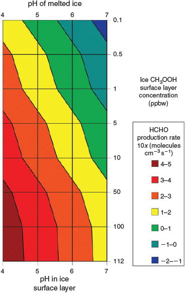
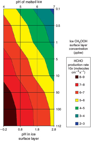
Model B(ii) is identical to Model B(i) but uses the assumption of enhanced acidic solute concentrations in the surface layer,[33] and therefore the assumed acidic solute concentrations lie in the millimolar range (pH –0.2–2.8) in the surface layer. It is again described by Fig. 2. Fig. 4 shows the variability in contribution to PHCHO from Eqn 7 across the range of acid solute and CH3OOH concentrations. The production rate varies between 6 × 10² and 6 × 10⁸ molecules cm–3 s–1, which is equivalent to a range in contributions to PHCHO of negligible to 350 % and a maximum enhancement in Δ[HCHO] of 2.3 ppbv. Given the large range of potential HCHO production rates and implausibly large upper limit indicated by Fig. 4 we attempt to introduce some constraints to limit the upper bounds. Based on assumption 5 and an upper limit on melted ice acid solute concentrations of 10 μM, we estimate that surface layer pH levels cannot be lower than 0.8. Introducing this constraint limits the contribution of Eqn 7 to PHCHO to between 5.6 × 10⁴ and 6.3 × 10⁷ molecules cm–3 s–1. There are two additional constraints: it is also not possible for the estimated PHCHO to exceed the empirically derived PHCHO; and most of PHCHO can be explained simply by physical desorption from ice grains. Therefore, using only a very generous limit, we suggest a remaining unidentified contribution to PHCHO cannot exceed 25 % of PHCHO. Thus, the estimated relative contributions to PHCHO from Eqn 7 cannot exceed this 25 % limit (4.3 × 10⁷ molecules cm–3 s–1). The upper limit flux estimate under pH 0.8 (6.3 × 10⁷ molecules cm–3 s–1) therefore exceeds those constraints by ~50 %, and therefore the lower limits of pH or the upper limits of CH3OOH concentration are unreasonable.
|
Having placed only loose external constraints upon both pH and CH3OOH concentration, which fail to suitably constrain the contribution to PHCHO we now try to select a plausible volume flux of HCHO from Eqn 7 and determine the lower bounds of pH (upper bounds for acidity) and CH3OOH that do not exceed this level. Considerable unquantified uncertainty is attached to model estimates of physically induced fluxes of HCHO,[15] yet the physical model can successfully explain the bulk of the observed HCHO. We therefore select an upper limit for the contribution from Eqn 7 that we believe cannot be ruled out by the physical model due to the remaining uncertainties attached to its flux estimates. Under these circumstances we chose to impose a reasonable upper limit: a flux magnitude of 12 % as a fraction of PHCHO, equivalent to 2.0 × 10⁷ molecules cm–3 s–1. We present ranges of CH3OOH concentration that satisfy this criteria at different pH levels: at a pH of 1.8 and at all CH3OOH concentrations fluxes are at or below this cut off, at pH 0.8 CH3OOH concentrations of 50 ppbw or below are reasonable, and at pH –0.2 only CH3OOH concentrations of 5 ppbw satisfy this criteria.
Part two: investigation of photochemical HCHO fluxes
Hutterli et al.[15] report a decrease in the total firn air HCHO concentration during shading experiments. We infer from this that the change in firn air concentration is due to a corresponding change in the total firn air HCHO volume flux (PHCHO), and results directly from the attenuation of sunlight. In addition, we infer that this leads to a consequent change in Δ[HCHO]. We define the portion of PHCHO that decreases during the shading experiments as PHCHO_PHOT, which is the photochemical flux of HCHO in the interstitial air. The aim of part two is to investigate PHCHO_PHOT. Assuming steady-state, Eqn 20 defines PHCHO_PHOT.

PHCHO_PHOT is calculated from the product of Δ[HCHO], the photochemical factor (PF), and the sum of FE, CT, and PT using Eqn 20. Δ[HCHO] = 1.24 × 10¹⁰ molecules cm–3 (650 pptv), PF can at most equal 0.2, and the sum of FE, CT and PT is 0.0139 s–1 to 3 s.f. The empirically derived value of PHCHO_PHOT is therefore 3.42 × 10⁷ molecules cm–3 s–1 to 3 s.f. We subsequently round it to 2 s.f. and conclude that photochemical losses of HCHO are small compared to the losses due to diffusion driven transport. We conduct a range of sensitivity studies (within three scenarios) to test various assumptions. Using the same framework used in Part One, we then derive different modelled values of PHCHO_PHOT and finally make a comparison to the empirically derived maximum possible value of PHCHO_PHOT (i.e. 4 × 10⁷ molecules cm–3 s–1). This comparison is rather limited by the large uncertainties on the empirically derived value of PHCHO_PHOT, so we can only provide an indication as to the level of consistency between the estimated and observed values. Note that only assumptions 1 and 2 from Part One are relevant to this set of analyses. The empirically derived PHCHO_PHOT is then compared to reported laboratory photochemical production rates of HCHO within snow. Additionally, PHCHO_PHOT is directly compared to the total interstitial air volume flux rate PHCHO (1.7 × 10⁸ molecules cm–3 s–1) within the existing theoretical framework presented for Models A, B(i), and B(ii) in Part One.
The laboratory work of Grannas et al.[17] provides photochemical production rates of HCHO within South Pole snow. The analysis reported directly implicates NO3– in the photochemical production of HCHO, probably by the OH• oxidation of OM. Note that H2O2 photolysis is also an important OH• source as it dominates the snowpack generation of OH•.[21,22] Grannas et al.[17] indicates that the rate of HCHO production within a block of South Pole snow was 8.4 × 10⁹ molecules cm–3 s–1. This production rate conflicts with the derived value of PHCHO_PHOT suggested by observations of Hutterli et al.[15] (i.e. 3.4 × 10⁷ molecules cm–3 s–1). This discrepancy is likely to be due to the fact that Grannas et al.[17] measured the total HCHO concentration within a melted liquid snow sample, and therefore accounts for HCHO production in the bulk and in the surface layer. However, the estimate of PHCHO_PHOT obtained by interpreting the observations in Hutterli et al.[15] is for the volume flux in the interstitial air due to photochemical production of HCHO on the surface of ice grains rather than the production on the surface and in the bulk. We discussed previously that Yabushita et al.[24] showed the potential importance of the location of the OH• source within the ice structure. For instance, their work implies that only the OH• produced in the top most ice monolayers may partake in either gas phase or surface layer chemistry. This therefore implies that the inconsistency between laboratory and field measurements could also be due to the removal of the potential spatial separation between the OH• sources and OM in a melted sample (see discussion in scenario 3 below). There are three quantities required to calculate the photochemical production rates of HCHO in the snowpack: (1) the OM concentration; (2) the rate constant for the reaction between OH• and OM and (3) and the OH• concentration.
The estimate of OM concentration (0.4 mg carbon L–1) was derived from the bulk OM concentration reported for South Pole snow.[17] The molarity of the OM is dependent upon the OM molecular weight, which is in turn dependent upon the chemical nature of the OM. No speciation of the South Pole OM exists,[17] but in the case of the other snowpacks analysed in Grannas et al.[17] the OM consisted partly of oligomeric phytochemicals. We select acetophenone and methoxybenzene as analogues for the OM based partly on their structural similarities to oligomeric phyto-chemicals and because of the availability of kinetic data. The molecular weights of acetophenone at 120 (96 for carbon only) and methoxybenzene at 108 (84 for carbon only) allow us to calculate the molar concentrations later in each scenario. The OM concentration of 0.4 mg carbon L–1 is expressed as the melted snow OM concentration and we must therefore account for the change in volume between melted and frozen snowpack in order to estimate snow OM concentration and molarity. We assume that the frozen snow volume is 30 % of the melted snow volume, which is equivalent to a snow density of 0.3 g cm–3.[33]
The aqueous phase rate coefficients for the reaction of OH• with acetophenone (6.5 × 1012 cm3 mol–1 s–1) and methoxybenzene (5.4 × 1012 cm3 mol–1 s–1) were obtained from the Radiation Laboratory database (http://www.rcdc.nd.edu/compilations/Hydroxyl/OH.htm, accessed July 2010). We henceforth refer to these rates in molecular units: for acetophenone this is 1.1 × 10⁻¹¹ cm3 molecules–1 s–1 and for methoxybenzene this is 9.0 × 10⁻¹² cm3 molecules–1 s–1. There is a lack of data regarding reaction coefficients on ice and we therefore assume that aqueous phase rate coefficients will adequately describe the reaction rate occurring on ice surfaces.
We use the steady-state approximation to calculate the OH• concentration in the surface layer. The OH• steady-state production terms from NO3– and H2O2 photolysis (Eqns 1, 2 and 5) were derived from France et al.[22] France et al.[22] report integrated snowpack column OH• production rates for both NO3– and H2O2 photolysis. We convert the column production rate into a volume flux at 10 cm of depth by solving for F(OH•)0, the OH• volume flux at the top of the snowpack, in Eqn 21.
where F(OH•)0 is the OH• production rate at the top of the snowpack, d is the depth in the snowpack in centimetres, de is the actinic flux e-folding depth within the snowpack and F(OH) is the integrated column OH• production rate in the snowpack. F(OH•) in the case of NO3– and H2O2 at the South Pole with a zenith angle of 66.5° is 2 × 10⁻⁹ μM cm–2 s–1 (1.2 × 10⁹ molecules cm–2 s–1) and 5 × 10⁻⁸ μM cm–2 s–1 (3 × 10¹⁰ molecules cm–2 s–1).[22] Measurements of actinic flux within the snowpack at Dome C identify an e-folding depth of ~10 cm, which we assume is valid for the South Pole.[38] We assume the photochemically active region of the snowpack extends over a 30-cm region below the surface based on those same measurements made at Dome C,[38] and solve for F(OH•)0 on this basis. Using F(OH•) for both NO3– and H2O2 we determine separate solutions of F(OH•)0 and in turn for F(OH•)d, the OH• production rate at depth d over a 1-cm thickness expressed in molecules per centimetre cubed per second, in Eqn 22.
Using this method we estimate respective values of F(OH•)0 and F(OH•)d (where d = 10 cm) for NO3– to be 1.3 × 10⁸ and 4.9 × 10⁷ molecules cm–3 s–1 and for H2O2 to be 3.3 × 10⁹ and 1.2 × 10⁹ molecules cm–3 s–1. Using firn air mixing ratios for other gas phase species we determine other OH• production terms, but find that NO3– and H2O2 photolysis dominates other production terms by two orders of magnitude. The calculated OM loss terms were in turn combined with the loss terms from the reaction of OH• with NOx, CH4, CO, oxygenated volatile organic compounds (OVOCs) and NMHCs,. We find that the Eqn 3 loss term dominates the other species loss terms by between one and five orders of magnitude depending on the assumed OM in the specific scenario. Within this treatment of the OH• losses we implicitly assume that the losses across both phases can be combined. This is justified because the OH• loss term is dominated by the losses due to OM, because OH• is produced within the surface layers of the ice, and because the OM is distributed in the surface layers of the ice. Thus, the OH• loss term is largely driven by a process occurring close to its production, and the OH• in the interstitial air can still react with the OM present on the exterior of ice grains.
Three scenarios were investigated using different means of estimating the OM and OH• concentrations available to react and produce HCHO capable to being released to the interstitial air.
-
We conduct a sensitivity study assuming a range of OM concentrations to determine how OM concentration affects HCHO production from Eqn 3. It is assumed that all of the OM is available to undergo reaction and that it is distributed on the surfaces of the ice grains and thus any HCHO produced photochemically can be released rapidly. The latter point seems plausible for polycyclic aromatic hydrocarbons.[39]
-
Using only the reported melted snow OM concentration (0.4 mg carbon L–1) we estimate a modified OM concentration to account for the particulate nature of the OM as reported in Grannas et al.,[17] thus creating an effective OM concentration at the surface of OM particles. Effective surface concentrations were derived using the size distributions reported in Grannas et al.[17] to yield a range of production rates of HCHO from Eqn 3. The steady-state OH• concentrations were recalculated to account for the differences in loss rate by Eqn 3.
-
Within this scenario, we only show results using acetophenone, we use an OM particle size of 0.035 μm and a melted snow OM concentration of 0.4 mg carbon L–1. We only used acetophenone in this analysis in order to simplify the analysis and reduce the number of results presented. The production rates of OH• were reduced compared to scenarios 1 and 2. These reductions are in-line with the experimental evidence presented by Yabushita et al.,[24] which show that OH• formed within the bulk ice likely reacts with H2O by Eqn 6a thereby becoming trapped in the bulk. It was suggested that only OH• produced in the outer most 3–4 monolayers of water ice is able to partake in gas phase or surface chemistry. We therefore assume that only the portion of OH• produced in the outer monolayers can react with OM in the surface layer. A range of sensitivity tests were developed to investigate the importance of OH• loss in bulk ice.
For the sake of simplicity the production of HCHO from CH3OOH oxidation by Eqn 10 is ignored in the following scenarios due to its insignificant contribution to HCHO production at the South Pole.
Scenario 1
We conducted a sensitivity analysis using four OM concentrations over the concentration range of 4 × 10⁻² to 8 × 10⁻¹ mg carbon L–1, and apply the volume ratio between frozen snow and melted snow (0.3) in concert with the carbon molecular masses. For both acetophenone and methoxybenzene we estimate a range of molar concentrations of OM within snow: 1.3 × 10⁻¹⁰–2.5 × 10⁻⁹ mol cm–3 and 1.4 × 10⁻¹⁰–2.9 × 10⁻⁹ mol cm–3. Henceforth, we refer to the OM concentrations in molecular units; thus, the concentrations are 7.8 × 10¹³–1.5 × 10¹⁵ moleclues cm–3 for acetophenone and 8.4 × 10¹³–1.7 × 10¹⁵ moleclues cm–3 for methoxybenzene.
Because we assume that the OM is distributed on the surface of ice grains these results estimate the amount of HCHO produced from the surface of ice grains. Two ranges of OH• loss terms were then derived for the reaction between OH• and acetophenone and for methoxybenzene using these different OM concentrations and the reaction rates quoted earlier. In both cases, the loss due to reaction with OM dominates the OH• loss term by between three and five orders of magnitude, i.e. 7.7 × 10² to 1.6 × 10⁴ s–1 v. 0.73 s–1 from other contributions. Using Eqn 23 and F(OH•)10 calculated above that incorporates OH• production from NO3– and H2O2 photolysis at a depth of 10 cm, we calculate two steady-state OH• concentration ranges of 7.8 × 10⁴ to 1.6 × 10⁶ molecules cm–3 s–1 (acetophenone) and 8.3 × 10⁴ to 1.7 × 10⁶ molecules cm–3 s–1 (methoxybenzene) depending on the OM concentration range and composition. Because the total loss term (L(OH)) is dominated by reaction with OM, and in turn multiplied by [OH•]ss to calculate PHCHO_PHOT, it should be clear that in this instance, and across the full OM concentration range, F(OH•)10 ≈ PHCHO_PHOT, which is equivalent to 1.27 × 10⁹ molecules cm–3 s–1.

OM concentrations would have to be reduced to below 9.0 × 10¹⁰ molecules cm–3 (1.5 × 10⁻¹³ mol cm–3) before the loss term of Eqn 3 is comparable with the sum of the other loss terms (e.g. NOx). Either analyses of snowpack OM concentrations or our treatment of the OM concentration would have to be significantly changed for OM not to be the dominant control of snowpack OH• concentrations in the model. These model derived estimates of PHCHO_PHOT from Eqn 3 are a factor of 28 greater than that implied by observations at the South Pole (i.e. 3.4 × 10⁷ molecules cm–3 s–1).[15] The use of these basic assumptions to calculate photochemical PHCHO_PHOT is therefore inadequate, and Scenario 1 compares poorly with the observations.
Scenario 2
We assume average particle sizes ranging between 0.01 and 5 μm, a melted snow OM concentration of 4 × 10⁻¹ mg carbon L–1, a particle composition and density equivalent to liquid acetophenone (1.028 g cm–3) and methoxybenzene (0.995 g cm–3), molecular lengths of 5.8 × 10⁻¹⁰ m (acetophenone) and 5.4 × 10⁻¹⁰ m (methoxybenzene) and molecular volumes of 1.9 × 10⁻²⁸ m3 (acetophenone) and 1.6 × 10⁻²⁸ m3 (methoxybenzene). Using these assumptions we derive ‘effective’ OM concentrations that are up to ~6.95 × 10⁻⁴ and 6.50 × 10⁻⁴ times smaller than the previously estimated concentrations for OM particle sizes of 5 μm and for both acetophenone and methoxybenzene respectively. Table 1 shows modelled estimates of PHCHO_PHOT produced using this new set of assumptions, while keeping the same steady-state treatment to derive the OH• concentrations. Note that the new OM concentrations are such that the OM loss term is significantly larger than the other loss terms. The estimates of PHCHO_PHOT due to Eqn 3 shown in Table 1 are not consistent with the value of PHCHO_PHOT implied by observations at the South Pole for any of the proposed particle sizes. In summary, these production rates are too large compared with the possible range of PHCHO_PHOT implied by observations at the South Pole (3.4 × 10⁷ molecules cm–3 s–1) and thus these assumptions alone are inadequate.

|
Scenario 3
We now carry out a sensitivity study to test how different distributions of NO3– and H2O2 within ice affect the production of OH• on the ice surface and interstitial air and in turn to see how this affects the production of HCHO. Four different assumptions regarding NO3– and H2O2 distribution within ice grains were used. It was assumed that H2O2 either had an even distribution throughout ice grains or that 4 % of the H2O2 was concentrated in the surface layer. We define the surface layer volume using the Boxe et al. treatment[33] thus yielding a surface-to-bulk volume ratio of 6.4 × 10⁻⁵. H2O2 is believed to be deposited by wet and dry deposition[15] and will therefore, in part, be accommodated directly into the bulk upon formation of snow at altitude. It was assumed that between 50 and 66 % of the NO3– was concentrated in the outer four monolayers. NOy at the South Pole is believed to undergo at least one cycle per summer season between snowpack NO3–, gas phase NOx and HNO3 to be deposited back in the snowpack. A significant portion of snowpack NO3– will have resulted from dry deposition of HNO3 of in situ photochemical origin. It is therefore assumed that NO3– is dry deposited onto ice grains and only undergoes partial accommodation into the bulk as the experimental work of Yabushita et al.[24] indicates that during dry deposition of HNO3 onto ice a portion of the NO3– resides on the surface. Furthermore, observations of the distribution of acid solutes within ice grains show a tendency for NO3– to accumulate at ice grain boundaries.[34,35] We also assume that OH• produced in the bulk can only penetrate through four monolayers to reach the surface[40] due to the effects of Eqn 6a. Note that the results in Table 1 showing effective OM concentrations for particles of acetophenone of 0.035 μm in diameter are relevant in this scenario. The results from the methoxybenzene calculations are within 10 % of the results from acetophenone and we do not show them below.
If 33 and 50 % of the snowpack NO3– is accommodated into the bulk ice and we assume an even distribution of H2O2 within the ice grains, the modelled estimates of PHCHO_PHOT are consistent with the empirically derived PHCHO_PHOT for the South Pole (Table 2). It therefore seems likely that only OH• produced near the uppermost layers of ice plays a role in HCHO production by reaction with OM at the ice grain surfaces and that a significant portion of the OH• produced within the bulk remains trapped there due to Eqn 6a.

|
Assuming the maximum possible value of PHCHO_PHOT, i.e. 4 × 10⁷ molecules cm–3 s–1, could be maintained indefinitely it would take 223 or 255 days to completely oxidise all of the OM assuming it was acetophenone or methoxybenzene respectively. Given that this time period greatly exceeds the time period over which intense summertime photochemistry occurs upon the Antarctic plateau it seems likely that the majority of deposited OM will be preserved within the snowpack. Assuming that the maximum possible PHCHO_PHOT could be maintained for a three month period centred on late December we estimate that between 35 and 40 % of the snowpack OM would be oxidised.
Temporal variability of HCHO fluxes
Regarding the chemical production of HCHO as per Eqn 7 involving CH3OOH, the CH3OOH rearrangement will primarily be controlled by the availability of CH3OOH and the pH of the snow.[30,31,33] The latter, in this case, will be controlled by the rate of deposition of acidic species to the snow, which is predominantly HNO3 deposition at the South Pole.[4] The availability of CH3OOH will be controlled by its flux into the boundary layer at the South Pole as it is not produced in significant amounts by in situ photochemistry.[9] The factors controlling the photochemical production of HCHO will be limited to the actinic flux, e.g. cloud cover and total ozone column. Ultimately, temperature will control the rate at which HCHO migrates from the ice phase to the firn air.[15,41] Further studies will be required to allow quantitative understanding of how these factors control the variability of heterogeneous chemical HCHO production.
A major controlling factor of fluxes driven by diffusion based transport, which is what we modelled here and is what is responsible for the majority of the HCHO flux observed at the South Pole,[15] is the concentration gradient between the firn and boundary layer. Thus, boundary layer variability of HCHO mixing ratios will have a decisive and direct control on the flux. For simplicity, we assumed the average HCHO boundary layer and firn air mixing ratios along with the mean fluxes that were observed, but more complex models would have to account for the variability in the flux due to changes in the gradient across the air–snow boundary. As a demonstration, we try to show how much the HCHO air–snow flux might vary first due to changes in the boundary layer mixing ratios. The observed HCHO mixing ratios in the South Pole boundary layer range from 27 to 184 pptv.[15] It isn’t inconceivable of course that HCHO boundary mixing ratios may vary to an even greater degree. However, coupling just this range with an assumed fixed firn air mixing ratio of 750 pptv, a rearrangement of Eqn 13, and our estimate of Vair implies VHCHO may vary from 1.5 × 10⁸ to 1.9 × 10⁸ molecules cm–3 s–1 solely due to changes in the mixing ratio in the overlying atmosphere, which gives a difference of up to 15 % from the mean observed value (1.7 × 10⁸ molecules cm–3 s–1).[15] Note that this derived range more than adequately accounts for the reported standard deviation (1 × 10⁷ molecules cm–3 s–1) about the mean HCHO flux.[15] Hutterli et al. do report a much wider range of flux variability that lies well beyond the standard deviation, and we surmise that those outlying fluxes can probably be explained through a combination of varying boundary layer dynamics, changes in temperature and consequent evaporation and re-adsoption and attenuation of actinic flux.
A further consideration is that the effect fluxes have on boundary layer mixing ratios is directly dependent on the boundary layer height. Shallower boundary layer heights and smaller mixing volumes favour higher mixing ratios. The flux variability may therefore ultimately be indirectly controlled by this external meteorological factor. Indeed, this same issue is discussed in the context of NOx in Davis et al.[3]
Although diffusion driven transport is the main way by which air is exchanged across the air–snow boundary, wind pumping does play a minor role. Thus, again, a more complex model that sought to model HCHO flux variabilities would have to consider this process because it can significantly increase the rate of air exchange.
Conclusion
The acid-catalysed processing of CH3OOH (via Eqn 7) according to the Yablokov mechanism to yield HCHO is a new potential source of HCHO within polar snowpacks. Using steady-state model simulations we showed that a flux magnitude of up to an equivalent of 12 % of PHCHO (2.0 × 10⁷ molecules cm–3 s–1) could be produced from Eqn 7 using plausible estimates of pH and CH3OOH concentrations in the ice surface layer. We suggest that a flux of this magnitude is sufficiently low such that it cannot be excluded by physically induced flux estimates with remaining considerable and unquantified uncertainty.[15] Surface layer concentration effects for acidic solutes are required to achieve sufficiently low pH in order to yield a non-negligible source of HCHO from the Yablokov mechanism. This mechanism may also explain the apparent lack of accumulated CH3OOH within South Pole snow despite Henry’s Law predicting CH3OOH at concentrations in excess of the analytical method’s limit of detection. Despite the presence of CH3OOH in the South Pole boundary layer and in the interstitial air, photolysis and reaction with OH• appear to be too slow to explain the majority of the observed photochemical flux of HCHO. For photolysis and reaction with OH• to be important, CH3OOH would have to accumulate in the snowpack up to and beyond detectable levels. Although we show a non-negligible volume flux from the Yablokov mechanism, our estimates of the flux are extremely imprecise due to a lack of more precise estimates of snow CH3OOH concentration and precise surface layer estimates of acid solute concentrations. Further study and observation will be required to precisely determine the volume flux magnitude. Indeed, without this work it will not be possible to resolve the wide uncertainties on the flux estimates and to satisfactorily resolve how it relates to the physical release model of Hutterli et al.[15]
We present three different scenarios to reconcile discrepancies between the modelled and observed snowpack photochemical production rate of HCHO. Scenario 3 provides the most comprehensive description of ice surface micro-environment conditions. Indeed, the predicted contributions to PHCHO_PHOT from scenario 3 using an even distribution of H2O2 within the ice are the most consistent with the size of PHCHO_PHOT implied by field measurements. Note that it is not possible to discriminate between the different possible distributions of NO3– within ice grains proposed within scenario 3 due to the large uncertainties on the PF parameter,[15] but PF would have to be approximately twice as large for the alternative H2O2 distribution to be valid. However, scenarios 1 and 2 are plainly excluded as being plausible due their large overestimate of PHCHO_PHOT. This study provides the necessary first step to simulating photochemical HCHO production before performing a study with greater detail using more advanced modelling techniques because it eliminates the most simplistic descriptions of the interaction between OH• and OM (such as in scenarios 1 and 2 in part two). It emphasises the requirement to consider the micro-environment in ice in a suitably accurate manner, and highlights the worth of the new laboratory measurements to improve understanding of surface layer photo-fragment dynamics. Using a simplistic model has allowed us to efficiently explore a wide range of different assumptions and uncertainty parameter space. However, further study is required to verify the assumptions of scenario 3 and to support more advanced modelling efforts. Specifically, more detailed speciated measurements of the OM need to be made at the South Pole in addition to measurements of OH• within the firn air. The distribution of OM within ice grains needs to be characterised to determine its separation from the interstitial air. The distribution of OH• precursors within ice grains also needs to be determined as this determines the surface OH• production efficiency. Laboratory studies need to be undertaken to investigate HCHO production on ice surfaces under a range of different conditions.
Although physical desorption adequately describes the bulk of the HCHO snowpack flux, consideration of the more minor chemical HCHO fluxes from within the snowpack is important for several reasons. HCHO fluxes have been demonstrated to influence local oxidation capacity and photochemistry in the South Pole boundary layer. The origin of two of the HCHO flux sources (Eqns 3, 7) could have implications for chemical tracers stored in the ice core record. First, the Yablokov mechanism presents a plausible hypothesis for why no CH3OOH has been observed above the limit of detection within snow at the South Pole despite Henry’s law predicting much higher concentrations. Second, the oxidation of OM by OH• proceeds at a sufficient rate at its maximum to affect OM preservation on the monthly timescale. In addition, demonstration of oxidation of OM by OH• produced from NO3– and H2O2 photolysis could have implications for the wider troposphere because these processes could feasibly occur in aerosols.
We would now like to summarise the assumptions used throughout this work, to characterise the uncertainties associated with these assumptions and to describe to what degree our results are sensitive to them. It should be noted that one objective of this work was to explore the uncertainty parameter space associated with some of these assumptions. We discuss the implications of the associated sensitivity studies below too.
We first address the overall theoretical structure used to describe the fluxes and production rates within the framework we use. The overall theoretical premise, using diffusion controlled transport combined with concentration gradients to drive air–snow fluxes under steady-state conditions, is sound. Indeed, we discounted wind pumping as being a major controlling factor on air–snow exchange for the empirical data we used, but it should not be excluded from more complex models. Furthermore, the steady-state assumption has also been validated empirically. Under the steady-state assumption, surface losses are discounted because at equilibrium, trace gas losses due to surface deposition onto ice grains are equal to the rate of re-evaporation. This assumption would break down under conditions of changing temperature though, which would have to be considered in a more complex model.
We relied on using the mean observed fluxes and concentration gradients to derive key parameters. We believe these mean observed fluxes and gradients are consistent with one another, and therefore we can adequately describe the mean case, but in using them we hugely simplified reality. This simplification was a necessary step in order to create a model that could feasibly address the parameter space of uncertainty. One further point of discussion is that the observed mixing ratios of HCHO and NOx within the firn air probably represent a lower bound because the measurement technique probably drew air into the snowpack from the boundary layer. We now discuss the uncertainty attached to the key parameter Vair. We showed that the uncertainty for the estimation of Vair could be as high as 17 %. Note too that this uncertainty extends to the variables that depend on it, i.e, FE, PHCHO and PHCHO_PHOT, and thus affect the proportions of PHCHO that our modelled fluxes can explain. Finally, the estimate of PF should be considered to carry significant uncertainty due the stated need in Hutterli et al.[15] to further verify the results of the shading experiments. However, the PF would have to be substantially different by an order of magnitude in order to invalidate the proposed mechanism of HCHO production in part two, scenario 3 and no plausible estimate of PF would validate scenarios 1 and 2.
The next issue is regarding our estimation of OH• in the snowpack in a steady-state. There is uncertainty in this estimation due to our reliance of the mean observed mixing ratios and concentrations of various OH• sinks (NOx, NMHCs, OM, etc.), due to our extrapolation of column OH• production rates to the production at 10-cm depth, and due to potential interaction with ice surfaces. Our results in part two are not directly sensitive to the steady-state OH• concentration that we derive, but they are strongly sensitive to the OH• production rate at the surface of ice grains because this limits the oxidation of OM in our model. The main source of uncertainty on the OH• production rate at the surface of ice grains is the distribution of H2O2 and NO3– within the ice, and we explored the model's sensitivity using a range of possible assumptions. Further work will be needed to reduce this uncertainty and further understand the distribution within ice of these OH• sources. There is however good support for our assumed NO3– distribution in ice from observations of its tendency to accumulate at ice grain boundaries and from laboratory measurements.[24,34,35] Future work seeking to address the oxidising capacity due to OH• within the snowpack through either measurements of its production and losses, or by direct observation would add support to this work too. The next uncertainty that we discuss again relates to scenario 3 in part two and it is the speciation and abundance of the OM detected in the snowpack. Although there is some uncertainty surrounding the OM composition, we showed that for two analogue species our results were not greatly sensitive to this issue. However, again in part two scenario 3, our results were sensitive to the concentrations of OM within the snowpack, which would affect our conclusions regarding PHCHO_PHOT. However, the OM concentrations would have to be two orders of magnitude lower than we considered for this to have a noticeable effect. We also used only one observation of OM within our model. Therefore, future work studying the amount of OM present within the South Pole snowpack would be beneficial. The results in part one were sensitive to the acid solute distribution, but there are strong theoretical grounds for supposing that acid solutes migrate to the ice grain boundaries. At various points in the work we used photolysis rates within the snowpack estimated using the TUV model for surface conditions at the South Pole. Although there is some uncertainty due to this assumption and these estimates likely represent an upper bound on the photolysis rates our results were not sensitive to them. Finally, in part one we were not able to constrain the concentration of CH3OOH within ice, and our results in part one B(ii) were sensitive to this as the sensitivity study showed. Further study with more sensitive instruments that can detect CH3OOH in melted ice samples will be required to lower this uncertainty.
Acknowledgements
P. D. Hamer and D. E. Shallcross thank NERC under the CHABLIS project for a studentship and British Antarctic Survey (BAS) for funding and for contribution to the publication fees. We thank Anna Jones at BAS and the colleagues within CHABLIS for their continued support and advice. Special thanks to Greg Huey for sharing the ISCAT 2000 field campaign data, M. Kawasaki and D. E. Shallcross thank the Daiwa-Adrian Foundation for an award to support this collaboration. This work is supported by a grant-in-aid from JSPS (20245005). The authors thank Centre National de Recherche Meteorologique, Meteo France, for funding.
References
[1] D. D. Davis, J. B. Nowak, G. Chen, M. Buhr, R. Arimoto, A. Hogan, F. Eisele, L. Maudlin, A. Hogan, D. Tanner, R. Shetter, B. Lefer, P. McMurry, Unexpected high levels of NO observed at South Pole. Geophys. Res. Lett. 2001, 28, 3625.| Unexpected high levels of NO observed at South Pole.Crossref | GoogleScholarGoogle Scholar | 1:CAS:528:DC%2BD3MXns1ykt70%3D&md5=3c813c4fb26291ca3afe62c4d3408247CAS |
[2] J. H. Crawford, D. D. Davis, G. Chen, M. Buhr, S. Oltmans, R. Weller, L. Mauldin, F. Eisele, R. Shetter, B. Lefer, R. Arimoto, A. Hogan, Evidence for the photochemical production of ozone at the South Pole surface. Geophys. Res. Lett. 2001, 28, 3641.
| Evidence for the photochemical production of ozone at the South Pole surface.Crossref | GoogleScholarGoogle Scholar | 1:CAS:528:DC%2BD3MXns1ykt7k%3D&md5=e023f1a44a795eb8b1c190dbc43d23d5CAS |
[3] D. D. Davis, G. Chen, M. Buhr, J. Crawford, D. Lenschow, B. Lefer, R. Shetter, F. Eisele, L. Maudlin, A. Hogan, South Pole NOx chemistry: an assessment of factors controlling variability and absolute levels. Atmos. Environ. 2004, 38, 5375.
| South Pole NOx chemistry: an assessment of factors controlling variability and absolute levels.Crossref | GoogleScholarGoogle Scholar | 1:CAS:528:DC%2BD2cXntVCqu7g%3D&md5=d50374097e85ede14b0fd338e0189c7dCAS |
[4] J. E. Dibb, L. G. Huey, D. L. Slusher, D. J. Tanner, Soluble reactive nitrogen oxides at South Pole during ISCAT 2000. Atmos. Environ. 2004, 38, 5399.
| Soluble reactive nitrogen oxides at South Pole during ISCAT 2000.Crossref | GoogleScholarGoogle Scholar | 1:CAS:528:DC%2BD2cXntVCqu7Y%3D&md5=57f02b0f89ab7e3e12d62689425aba8aCAS |
[5] L. G. Huey, D. J. Tanner, D. L. Slusher, J. E. Dibb, R. Arimoto, G. Chen, D. D. Davis, M. P. Buhr, J. B. Nowak, R. L. Mauldin, CIMS measurements of HNO3 and SO2 at the South Pole during ISCAT 2000. Atmos. Environ. 2004, 38, 5411.
| CIMS measurements of HNO3 and SO2 at the South Pole during ISCAT 2000.Crossref | GoogleScholarGoogle Scholar | 1:CAS:528:DC%2BD2cXntVCqu7c%3D&md5=17b67b5bb4c16613b0669c7030afa92fCAS |
[6] R. L. Mauldin, F. L. Eisele, D. J. Tanner, E. Kosciuch, R. Shetter, B. Lefer, S. R. Hall, J. B. Nowak, M. Buhr, G. Chen, P. Wang, D. D. Davis, Measurements of OH, H2SO4, and MSA at the South Pole during ISCAT. Geophys. Res. Lett. 2001, 28, 3629.
| Measurements of OH, H2SO4, and MSA at the South Pole during ISCAT.Crossref | GoogleScholarGoogle Scholar | 1:CAS:528:DC%2BD3MXns1ykt7o%3D&md5=316d36cc42002b61c92f9973f2003f5eCAS |
[7] G. Chen, D. D. Davis, J. Crawford, J. B. Nowak, F. Eisele, R. L. Mauldin, D. Tanner, M. Buhr, R. Shetter, B. Lefer, R. Arimoto, A. Hogan, D. Blake, An investigation of South Pole HOx chemistry: comparison of model results with ISCAT observations. Geophys. Res. Lett. 2001, 28, 3633.
| An investigation of South Pole HOx chemistry: comparison of model results with ISCAT observations.Crossref | GoogleScholarGoogle Scholar | 1:CAS:528:DC%2BD3MXns1ykt7s%3D&md5=03a8d275e0f1e60ca84c710866f24513CAS |
[8] G. Chen, D. Davis, J. Crawford, L. M. Hutterli, L. G. Huey, D. Slusher, L. Maudlin, F. Eisele, D. Tanner, J. Dibb, A reassessment of HOx South Pole chemistry based on observations recorded during ISCAT 2000. Atmos. Environ. 2004, 38, 5451.
| A reassessment of HOx South Pole chemistry based on observations recorded during ISCAT 2000.Crossref | GoogleScholarGoogle Scholar | 1:CAS:528:DC%2BD2cXntVGjsrw%3D&md5=756005dde095cff4b1ac6dff19a13c3eCAS |
[9] P. D. Hamer, D. E. Shallcross, M. M. Frey, Modelling the impact of oxygenated VOC and meteorology upon the boundary layer photochemistry at the South Pole. Atmos. Sci. Lett. 2007, 8, 14.
| Modelling the impact of oxygenated VOC and meteorology upon the boundary layer photochemistry at the South Pole.Crossref | GoogleScholarGoogle Scholar |
[10] P. D. Hamer, A. Yabushita, M. Kawasaki, D. E. Shallcross, Modelling the impact of possible snowpack emissions of O(3P) and NO2 on photochemistry in the South Pole boundary layer. Environ. Chem. 2008, 5, 268.
| Modelling the impact of possible snowpack emissions of O(3P) and NO2 on photochemistry in the South Pole boundary layer.Crossref | GoogleScholarGoogle Scholar | 1:CAS:528:DC%2BD1cXhtVWitLbM&md5=0274665642632bf239f1c05012b98536CAS |
[11] A. E. Jones, R. Weller, E. W. Wolff, H. W. Jacobi, Speciation and rate of photochemical NO and NO2 production in Antarctic snow. Geophys. Res. Lett. 2000, 27, 345.
| Speciation and rate of photochemical NO and NO2 production in Antarctic snow.Crossref | GoogleScholarGoogle Scholar | 1:CAS:528:DC%2BD3cXhtV2lurk%3D&md5=54fbd203bd3036e69d58d46ecda567d1CAS |
[12] E. S. N. Cotter, A. E. Jones, E. W. Wolff, S. J. B. Bauguitte, What controls photochemical NO and NO2 production from snow? Laboratory investigation assessing the wavelength and temperature dependence. J. Geophys. Res. 2003, 108, 4147.
| What controls photochemical NO and NO2 production from snow? Laboratory investigation assessing the wavelength and temperature dependence.Crossref | GoogleScholarGoogle Scholar |
[13] A. Yabushita, D. Iida, T. Hama, M. Kawasaki, Release of oxygen atoms and nitric oxide molecules from the ultraviolet photodissociation of nitrate adsorbed on water ice films at 100 K. J. Phys. Chem. 2007, 111, 8629.
| Release of oxygen atoms and nitric oxide molecules from the ultraviolet photodissociation of nitrate adsorbed on water ice films at 100 K.Crossref | GoogleScholarGoogle Scholar | 1:CAS:528:DC%2BD2sXptVejsrk%3D&md5=05d6a541475fb84dd1ea9c7b71011ec7CAS |
[14] K. Riedel, R. Weller, O. Schrems, Variability of formaldehyde in the Antarctic troposphere. Phys. Chem. Chem. Phys. 1999, 1, 5523.
| Variability of formaldehyde in the Antarctic troposphere.Crossref | GoogleScholarGoogle Scholar | 1:CAS:528:DC%2BD3cXos1akug%3D%3D&md5=6cf790ff5daaaa5b103ccc8f8ef78df0CAS |
[15] M. A. Hutterli, J. R. McConnell, G. Chen, R. C. Bales, D. D. Davis, D. H. Lenschow, Formaldehyde and hydrogen peroxide in air, snow and interstitial air at South Pole. Atmos. Environ. 2004, 38, 5439.
| Formaldehyde and hydrogen peroxide in air, snow and interstitial air at South Pole.Crossref | GoogleScholarGoogle Scholar | 1:CAS:528:DC%2BD2cXntVGjsr8%3D&md5=c0fbda57c9f361862db150957b4ba7ebCAS |
[16] A. L. Sumner, P. B. Shepson, Snowpack production of formaldehyde and its effect on the Arctic troposphere. Nature 1999, 398, 230.
| Snowpack production of formaldehyde and its effect on the Arctic troposphere.Crossref | GoogleScholarGoogle Scholar | 1:CAS:528:DyaK1MXitVGksro%3D&md5=395897ce67c8efef44874b13b12c7590CAS |
[17] A. M. Grannas, P. B. Shepson, T. R. Filley, Photochemistry and nature of organic matter in Arctic and Antarctic snow. Global Biogeochem. Cycles 2004, 18, GB1006.
| Photochemistry and nature of organic matter in Arctic and Antarctic snow.Crossref | GoogleScholarGoogle Scholar |
[18] L. Chu, C. Anastasio, Quantum yields of hydroxyl radical and nitrogen dioxide from the photolysis of nitrate on ice. J. Phys. Chem. A 2003, 107, 9594.
| Quantum yields of hydroxyl radical and nitrogen dioxide from the photolysis of nitrate on ice.Crossref | GoogleScholarGoogle Scholar | 1:CAS:528:DC%2BD3sXot1Khs7c%3D&md5=bc2363536a71918f53c7b18feba0c456CAS |
[19] J. Mack, J. R. Bolton, Photochemistry of nitrite and nitrate in aqueous solution: a review. J. Photochem. Photobiol. Chem. 1999, 128, 1.
| Photochemistry of nitrite and nitrate in aqueous solution: a review.Crossref | GoogleScholarGoogle Scholar | 1:CAS:528:DyaK1MXnvVyqsbY%3D&md5=ab60279617e349a620db5aaf70630e9cCAS |
[20] G. Mark, H. G. Korth, H. P. Schuchmann, C. v. Sonntag, The photochemistry of aqueous nitrate ion revisited. J. Photochem. Photobiol. Chem. 1996, 101, 89.
| The photochemistry of aqueous nitrate ion revisited.Crossref | GoogleScholarGoogle Scholar | 1:CAS:528:DyaK2sXit1Kqurw%3D&md5=774502f94fecb8b691c6e48fd670b663CAS |
[21] L. Chu, C. Anastasio, Formation of hydroxyl radical from the photolysis of frozen hydrogen peroxide. J. Phys. Chem. A 2005, 109, 6264.
| Formation of hydroxyl radical from the photolysis of frozen hydrogen peroxide.Crossref | GoogleScholarGoogle Scholar | 1:CAS:528:DC%2BD2MXlsF2ms7Y%3D&md5=f6bd352c74f3aa72be0b72a3c978181fCAS | 16833967PubMed |
[22] J. L. France, M. D. King, J. Lee-Taylor, Hydroxyl (OH) radical production rates in snowpacks from photolysis of hydrogen peroxide (H2O2) and nitrate (NO3–). Atmos. Environ. 2007, 41, 5502.
| Hydroxyl (OH) radical production rates in snowpacks from photolysis of hydrogen peroxide (H2O2) and nitrate (NO3–).Crossref | GoogleScholarGoogle Scholar | 1:CAS:528:DC%2BD2sXns1KqsL4%3D&md5=fdd5310cd0f9954f3a132d91af16ae4fCAS |
[23] X. Zhou, K. Mopper, Photochemical production of low-molecular-weight carbonyl compounds in seawater and surface microlayer and their air-sea exchange. Mar. Chem. 1997, 56, 201.
| Photochemical production of low-molecular-weight carbonyl compounds in seawater and surface microlayer and their air-sea exchange.Crossref | GoogleScholarGoogle Scholar | 1:CAS:528:DyaK2sXhsFCmu7s%3D&md5=ebe9044c3365ad467656b4fcd4ab2c30CAS |
[24] A. Yabushita, D. Lida, T. Hama, M. Kawasaki, Observation of OH radicals ejected from water ice surface in the photoirradiation of nitrate adsorbed on ice at 100 K. J. Phys. Chem. A 2008, 112, 9763.
| Observation of OH radicals ejected from water ice surface in the photoirradiation of nitrate adsorbed on ice at 100 K.Crossref | GoogleScholarGoogle Scholar | 1:CAS:528:DC%2BD1cXhtVymtL%2FK&md5=28f93cd87e7cc3ec1ab23f6cde7ffcefCAS | 18778045PubMed |
[25] T. Uchimaru, A. Chandra, S. Tsuzuki, M. Sugie, A. Sekiya, Ab initio investigation on the reaction path and rate for the gas-phase reaction of HO + H2O ↔ H2O + OH. J. Comput. Chem. 2003, 24, 1538.
| Ab initio investigation on the reaction path and rate for the gas-phase reaction of HO + H2O ↔ H2O + OH.Crossref | GoogleScholarGoogle Scholar | 1:CAS:528:DC%2BD3sXntFent7w%3D&md5=45ed3bfbcc247f7e9f78cc7c600d7f7aCAS | 12925998PubMed |
[26] S. Andersson, A. Al-Halabi, G.-J. Kroes, E. F. v. Dishoeck, Molecular-dynamics study of photodissociation of water in crystalline and amorphous ices. J. Chem. Phys. 2006, 124, 064715.
| Molecular-dynamics study of photodissociation of water in crystalline and amorphous ices.Crossref | GoogleScholarGoogle Scholar |
[27] P. Cooper, J. Abbatt, Heterogeneous interactions of OH and HO2 radicals with surfaces characteristic of atmospheric particulate matter. J. Phys. Chem. A 1996, 100, 2249.
| Heterogeneous interactions of OH and HO2 radicals with surfaces characteristic of atmospheric particulate matter.Crossref | GoogleScholarGoogle Scholar | 1:CAS:528:DyaK28Xks1OntQ%3D%3D&md5=a11b43d49f2fa69f07a66aa85a07ea8dCAS |
[28] M. M. Frey, R. W. Stewart, J. R. McConnell, R. C. Bales, Atmospheric hydroperoxides in West Antarctica: Links to stratospheric ozone and atmospheric oxidation capacity. J. Geophys. Res. – D. Atmospheres 2005, 110, D23301.
| Atmospheric hydroperoxides in West Antarctica: Links to stratospheric ozone and atmospheric oxidation capacity.Crossref | GoogleScholarGoogle Scholar |
[29] K. Riedel, R. Weller, O. Schrems, G. Konig-Langlo, Variability of tropospheric hydroperoxides at a coastal surface site in Antarctica. Atmos. Environ. 2000, 34, 5225.
| Variability of tropospheric hydroperoxides at a coastal surface site in Antarctica.Crossref | GoogleScholarGoogle Scholar | 1:CAS:528:DC%2BD3cXovVWlu78%3D&md5=2b4bad202c22d6c6bce79349cdaaee9cCAS |
[30] V. A. Yablokov, The mechanisms of the rearrangements of peroxides. Russ. Chem. Rev. 1980, 49, 833.
| The mechanisms of the rearrangements of peroxides.Crossref | GoogleScholarGoogle Scholar |
[31] M. B. Smith, J. March, March’s Advanced Organic Chemistry 2001 (Wiley: Hoboken, NJ)
[32] M. Legrand, P. Mayewski, Glaciochemistry of polar ice cores: a review. Rev. Geophys. 1997, 35, 219.
| Glaciochemistry of polar ice cores: a review.Crossref | GoogleScholarGoogle Scholar | 1:CAS:528:DyaK2sXns1Slt7w%3D&md5=4497f33077f628f7a529c8d969481851CAS |
[33] C. S. Boxe, A. Saiz-Lopez, Multiphase modeling of nitrate photochemistry in the quasi-liquid layer (QLL): implications for NOx release from the Arctic and coastal Antarctic snowpack. Atmos. Chem. Phys. 2008, 8, 4855.
| Multiphase modeling of nitrate photochemistry in the quasi-liquid layer (QLL): implications for NOx release from the Arctic and coastal Antarctic snowpack.Crossref | GoogleScholarGoogle Scholar | 1:CAS:528:DC%2BD1cXhtlCnurrN&md5=1819688f4251410dda2b9ef0cd0c33c6CAS |
[34] H. Fukazawa, K. Sugiyama, S. Mae, H. Narita, T. Hondoh, Acid ions at triple junction of Antarctic ice observed by Raman scattering. Geophys. Res. Lett. 1998, 25, 2845.
| Acid ions at triple junction of Antarctic ice observed by Raman scattering.Crossref | GoogleScholarGoogle Scholar | 1:CAS:528:DyaK1cXlsF2msb8%3D&md5=110e17dfd8b4dfa4bb910fd07a5ea580CAS |
[35] R. Mulvaney, E. W. Wolff, K. Oates, Sulphuric acid at grain boundaries in Antarctic ice. Nature 1988, 331, 247.
| Sulphuric acid at grain boundaries in Antarctic ice.Crossref | GoogleScholarGoogle Scholar | 1:CAS:528:DyaL1cXotFGltg%3D%3D&md5=5a82a507e7b1f280066562e51dc4254eCAS |
[36] S. P. Oncley, M. Buhr, D. H. Lenschow, D. D. Davis, S. R. Semmer, Observations of summertime NO fluxes and boundary-layer height at the South Pole during ISCAT 2000 using scalar similarity. Atmos. Environ. 2004, 38, 5389.
| Observations of summertime NO fluxes and boundary-layer height at the South Pole during ISCAT 2000 using scalar similarity.Crossref | GoogleScholarGoogle Scholar | 1:CAS:528:DC%2BD2cXntVCqu7k%3D&md5=2af8f38629e2a757371f44234d1a6f34CAS |
[37] M. E. Jenkin, S. M. Saunders, M. J. Pilling, The tropospheric degradation of volatile organic compounds: a protocol for mechanism development. Atmos. Environ. 1997, 31, 81.
| The tropospheric degradation of volatile organic compounds: a protocol for mechanism development.Crossref | GoogleScholarGoogle Scholar | 1:CAS:528:DyaK28XntVOnt78%3D&md5=b7649e0a9b82efaeff8d90871fc5917fCAS |
[38] J. L. France, M. D. King, M. M. Frey, J. Erbland, G. Picard, A. MacArthur, J. Savarino, Snow optical properties at Dome C, Antarctica – implications for snow emissions and snow chemistry of reactive nitrogen. Atmos. Chem. Phys. Discuss. 2011, 11, 11 959.
| Snow optical properties at Dome C, Antarctica – implications for snow emissions and snow chemistry of reactive nitrogen.Crossref | GoogleScholarGoogle Scholar |
[39] A. M. Grannas, A. E. Jones, J. Dibb, M. Ammann, C. Anastasio, H. J. Beine, M. Bergin, J. Bottenheim, C. S. Boxe, G. Carver, G. Chen, J. H. Crawford, F. Dominé, M. M. Frey, M. I. Guzmán, D. E. Heard, D. Helmig, M. R. Hoffmann, R. E. Honrath, L. G. Huey, M. Hutterli, H. W. Jacobi, P. Klán, B. Lefer, J. McConnell, J. Plane, R. Sander, J. Savarino, P. B. Shepson, W. R. Simpson, J. R. Sodeau, R. von Glasow, R. Weller, E. W. Wolff, T. Zhu, An overview of snow photochemistry: evidence, mechanism and impacts. Atmos. Chem. Phys. 2007, 7, 4329.
| An overview of snow photochemistry: evidence, mechanism and impacts.Crossref | GoogleScholarGoogle Scholar | 1:CAS:528:DC%2BD2sXhtlWiurbJ&md5=553bd763d13bdd229972dd3e09eeaa03CAS |
[40] S. Andersson, E. F. v. Dishoeck, Photodesorption of water ice. A molecular dynamics study. Astron. Astrophys. 2008, 491, 907.
| Photodesorption of water ice. A molecular dynamics study.Crossref | GoogleScholarGoogle Scholar | 1:CAS:528:DC%2BD1MXhtFSltLs%3D&md5=fe1e86a751f4f6d3f5c3ff8956ca1106CAS |
[41] M. A. Hutterli, J. R. McConnell, G. Chen, R. C. Bales, D. D. Davis, D. H. Lenschow, Atmosphere-to-snow-to-firn transfer studies of HCHO at Summit, Greenland. Geophys. Res. Lett. 1999, 26, 1691.
| Atmosphere-to-snow-to-firn transfer studies of HCHO at Summit, Greenland.Crossref | GoogleScholarGoogle Scholar | 1:CAS:528:DyaK1MXkt1Ggtr4%3D&md5=6f0d0755c718ec26777b70a8bcb873f3CAS |