

Using species distribution models to infer potential climate change-induced range shifts of freshwater fish in south-eastern Australia
Nick Bond A B C F , Jim Thomson A , Paul Reich A D and Janet Stein EA School of Biological Sciences, Monash University, Clayton, Vic. 3800, Australia.
B eWater Cooperative Research Centre, Monash University, Clayton, Vic. 3800, Australia.
C Present address: Australian Rivers Institute, Griffith University, Nathan, Qld 4111, Australia.
D Arthur Rylah Institute for Environmental Research, Department of Sustainability and Environment, Heidelberg, Vic. 3084, Australia.
E The Fenner School of Environment and Society, Australian National University, Canberra, ACT 0200, Australia.
F Corresponding author. Email: n.bond@griffith.edu.au
Marine and Freshwater Research 62(9) 1043-1061 https://doi.org/10.1071/MF10286
Submitted: 16 November 2010 Accepted: 11 June 2011 Published: 21 September 2011
Journal Compilation © CSIRO Publishing 2011 Open Access CC BY-NC-ND
Abstract
There are few quantitative predictions for the impacts of climate change on freshwater fish in Australia. We developed species distribution models (SDMs) linking historical fish distributions for 43 species from Victorian streams to a suite of hydro-climatic and catchment predictors, and applied these models to explore predicted range shifts under future climate-change scenarios. Here, we present summary results for the 43 species, together with a more detailed analysis for a subset of species with distinct distributions in relation to temperature and hydrology. Range shifts increased from the lower to upper climate-change scenarios, with most species predicted to undergo some degree of range shift. Changes in total occupancy ranged from –38% to +63% under the lower climate-change scenario to –47% to +182% under the upper climate-change scenario. We do, however, caution that range expansions are more putative than range contractions, because the effects of barriers, limited dispersal and potential life-history factors are likely to exclude some areas from being colonised. As well as potentially informing more mechanistic modelling approaches, quantitative predictions such as these should be seen as representing hypotheses to be tested and discussed, and should be valuable for informing long-term strategies to protect aquatic biota.
Additional keywords: bioclimatic model, conservation planning, environmental filters, hydrology, prediction, validation.
Introduction
With anticipated changes in climate regime, including changes in temperature, rainfall and runoff, there is an increasing emphasis on understanding how species distribution patterns may change, and how to incorporate this information into conservation and restoration planning (Thuiller 2007; Palmer et al. 2007). This has stimulated considerable debate about how best to predict potential distributional shifts, and, in particular, whether correlative species distribution models (SDMs) are appropriate for predicting range shifts, or whether more mechanistic approaches are required (Heikkinen et al. 2006; Thuiller 2007; Kearney and Porter 2009; Elith et al. 2010; Sinclair et al. 2010).
Whereas much of this debate pits correlative and mechanistic approaches against one another, an alternative view sees correlative models as a valuable means of establishing hypotheses and identifying important processes to consider when developing mechanistic models for unstudied organisms (Buckley et al. 2010). Befitting this view is the recent trend towards statistical-modelling techniques based on information theory (such as neural networks, regression trees and random forests). These approaches rely less on an underlying model structure than do traditional modelling tools and are well suited to capturing non-linear relationships and interactions among predictors, therefore lending themselves to generating novel insights into species–environment relationships (Olden et al. 2008; Elith and Leathwick 2009). Despite the fact that evidence for climate-change impacts on fish species distributions is still rare (Booth et al. 2011), recent application of SDM approaches suggests that future range shifts of freshwater biota may be substantial (e.g. Buisson and Grenouillet 2010; Elith et al. 2010; Lyons et al. 2010).
Climate and hydrologic regimes have long been recognised as important environmental filters operating on aquatic ecosystems. Numerous studies have demonstrated predictable relationships between hydro-climatic conditions and the distribution patterns of freshwater biota – especially fish and macroinvertebrates (e.g. Poff and Allan 1995; Leathwick et al. 2005; Growns and West 2008). In rivers, patterns of flow variability are a major driver of ecosystem structure and function, and thus changes in flow can have a strong impact on species occurrence patterns (e.g. Kennard et al. 2007; Bond et al. 2010). Studies examining the effects of climate change on patterns of stream flow (e.g. Poff et al. 1996; Gibson et al. 2005; CSIRO 2008) suggest potential for substantial changes not just in average runoff but also in the occurrence, frequency and timing of ecologically relevant flows such as cease-to-flow periods and overbank flows that inundate floodplain areas. There is thus a need to try and capture these aspects of hydrology in examining climate-change impacts in aquatic ecosystems and to provide robust predictions of changes in species distribution.
Here, we examine potential range shifts of freshwater fish species in Victoria in south-eastern Australia under a range of climate scenarios, and explore species–environment relationships to help elucidate important hydro-climatic drivers. We developed SDMs linking contemporary species distributions to average contemporary climatic, hydrologic and physiographic characteristics, and combined the resultant models with scenarios of drought and climate change to explore the likely long-term impacts of different climate scenarios on species distributions. We developed models for 43 freshwater species and explored the impacts of three (low, median and high temperature) scenarios for 2030.
As well as summarising the overall changes in distribution patterns of the 43 species, we also present more detailed results for three native species, namely river blackfish (Gadopsis marmoratus Richardson, 1848), golden perch (Macquaria ambigua Richardson, 1845) and flathead gudgeon (Philypnodon grandiceps (Krefft, 1864)), and one introduced species, brown trout (Salmo trutta Linnaeus, 1758), with the aim of highlighting the types of response functions displayed to strong hydro-climatic drivers for each species, and illustrating the geographic range shifts that may occur. These species occupy a range of habitats from cool-water perennial streams through to intermittent lowland streams and large floodplain rivers, and are thus illustrative of the types of responses displayed by other species. There are varying levels of existing information on physiological tolerances and traits of each species; in particular, there is much detailed work on the physiological tolerances of brown trout against which to contrast the observed associations arising from our correlative models.
Materials and methods
Fish distribution data
Survey records detailing species distribution data were drawn from the Victorian Department of Sustainability and Environment’s Aquatic Fauna Database (AFD), which holds records from sites across Victoria as far back as the late 1800s. We restricted our analysis to 3708 sites surveyed between 1980 and 2000 for which reliable location and sampling information were available, overcoming some of the problems associated with the reliability of (particularly early) records in these sorts of databases. AFD data were supplemented by more recent data collected between 2004 and 2006 from 769 sites across Victoria that were surveyed as part of the Murray–Darling Basin Sustainable Rivers Audit (SRA) and the Southern Basins Audit (SBA). SRA and SBA surveys used electrofishing (backpack-, bank- and/or boat-mounted units), whereas the AFD database records involved a range of methods, including electrofishing, nets and piscicides. Sites below large impoundments were excluded from our analyses because such reaches tend to hold fish communities that are markedly atypical of those expected on the basis of natural climate and hydrology (e.g. Pollino et al. 2004; Quist et al. 2005), which could lead to misleading modelled relationships. We also excluded sites for which the spatial coordinates could not be reconciled against other information such as stream name and other site information, indicating potential errors in location details. All data were converted to presence/absence for the modelling, and in total, 43 species were represented (Table 1). This included several estuarine species frequently encountered in freshwater environments, but did not distinguish between some taxa for which taxonomic uncertainties remain, including the Hypseleotris species complex (including H. klunzingeri and several undescribed species) and Galaxias olidus, which also consists of several as yet undescribed species.

|
Environmental data
The major source of environmental data was a digital elevation model (DEM)-derived stream network linked to a set of summary statistics on climate and catchment characteristics associated with each reach (Stein 2006). The stream network is derived from a 9″ DEM and includes more than 45 000 reaches across Victoria. Catchment and climate datasets linked to the stream network are described in more detail by (Stein 2006; Walsh et al. 2007), and indicators of catchment disturbance in Stein et al. (2002). Variables used in the modelling are summarised in Table 2.

|
As with similar studies, we attempted to restrict the set of environmental predictors used in the modelling to those for which a mechanistic link with fish occurrence could be identified (e.g. Leathwick et al. 2005), and further sought to focus on climate-related predictors to maximise model sensitivity to climate-change scenarios. A comparison of model structures did, however, show that the inclusion of elevation improved the fit of the models for a small number of species (especially estuarine taxa), while having very minor impacts on predictions and scenarios for other species. There was also a weaker than expected correlation between temperature and elevation (r = 0.65), and here we present results from models that include elevation.
Hydrologic data
Given the recognised importance of hydrology as an environmental filter on biotic distributions in south-eastern Australia (e.g. Growns and West 2008; Bond et al. 2010), information on the hydrologic regime of individual river reaches was seen as a key component of the environmental-data requirements for modelling climate-change impacts. Although there is an increasing emphasis on ecologically relevant aspects of the flow regime in studies of climate-change impacts on runoff (e.g. Gibson et al. 2005; CSIRO 2008), most such studies are based on summarising results from calibrated rainfall–runoff models, which can realistically only be calibrated for specific nodes in a river network, generally at gauged sites where calibration data are available. Although this approach produces detailed time-series of runoff, logistically it is not feasible to build these models at a density capable of representing hydrologic characteristics of the entire river network. An alternative approach is to develop regression models relating flow characteristics (flow indices) measured at a gauge with climate and upstream catchment characteristics, and to use these models to extrapolate hydrologic indices to other parts of the river network (Sinclair Knight Merz 2005; Sanborn and Bledsoe 2006). This approach provides insights into long-term stream-flow characteristics that can be combined with other catchment attribute data to develop SDMs (Lyons et al. 2010). Gauge data for use in the hydrologic modelling were drawn from 120 unregulated sites distributed across Victoria (see Kennard et al. 2010b, for gauge locations), with sufficient record length to adequately quantify hydrologic regimes – in this case more than 15 years (Kennard et al. 2010a). A small set of hydrologic indices, including mean daily flow, daily and annual coefficient of variation in flow volumes (daily and annual CVs), daily 10th (daily Q10) and 90th (daily Q90) percentile flows, and mean annual number of zero-flow days were included in the predictive modelling. As with the species distribution models themselves, hydrologic indices were modelled as a function of climate and catchment attributes in the catchment above each gauge (Table 2). As summarised in the results section, high flow events could not be modelled with sufficient reliability to be included in the fish predictive models. Clearly, this removes our capacity to identify the impact of altered high flow regimes on species distributions; however, this is partially offset by the fact that changes in low flow characteristics are critical hydrologic filters affecting in-channel riverine species distributions (Balcombe et al. 2011; Pratchett et al. 2011).
Climate scenarios
We examined the impacts of three climate-change scenarios (consisting of changes (δ) in temperature (T), precipitation (P) and evapotranspiration (Etw)). Scenarios corresponded to the low, median and high estimates of δT (+0.54°C, +0.85°C and +1.24°C) for 2030 from the SRES marker scenarios of IPCC (2001). Estimates of changes in P and Etw were drawn from a spreadsheet model accompanying Jones and Durack (2005), which presented lower, median and upper estimates of δP (–1.1%, –3.3%, –6.0%) and δEtw (+2.0%, +3.1%, +4.6%) in catchments across Victoria from 10 climate models scaled to the low, median and upper IPCC temperature scenarios. Changes in T, P and Etw were applied to baseline climate characteristics from the climate atlas of Australia (Bureau of Meteorology 2002).
The effects of climate change on species distributions were modelled by first running the statistical hydrology models to derive predicted hydrologic characteristics for each reach under each of the three scenarios. These derived hydrologic data were then combined with scenario climate data and fixed catchment attributes as input to the statistical models built using the historical climate and species-distribution data.
Statistical modelling
Statistical models for both hydrology and fish were built using boosted regression trees (BRTs; Elith et al. 2008). BRTs represent a form of model averaging, in which multiple models are combined for prediction and inference, thereby accounting for uncertainty in model structure. The BRT method combines large numbers of relatively simple regression-tree models in an adaptive fitting process (Friedman 2001). BRTs have strong predictive performance, are well suited to identifying important predictor variables, and capture non-linearity in the response to individual predictors, and interactions among predictors (Elith et al. 2008). BRT models were built using the gbm package (Ridgeway 2007) in R (R Development Core Team 2009), with the default shrinkage (‘learning rate’ in Elith et al. 2008) value of 0.001 and the maximum interaction depth (‘tree complexity’) set to 5. Initial BRT models were based on 4000 trees, and the out-of-bag (OOB) estimate of predictive performance was used to select the optimal number of trees for each species. OOB estimates of error rate are based on bootstrap sampling using a random subset of records (50%) as training data for each iteration.
Model fit was assessed on the basis of the residual error (R2) in the case of continuous response variables, and on the basis of the area under receiver operator-characteristic curves (area-under-curve; AUC) for binomial variables. The receiver operator curves indicate the relative proportions of correctly and incorrectly classified predictions over a wide range of probability threshold levels, and are therefore independent of the (arbitrary) choice of a threshold probability to determine whether or not a site is predicted to be occupied (Burgman 2005). AUC values are also largely independent of species prevalence (Pearce and Ferrier 2000). AUC values >0.7 are generally deemed to indicate adequate discrimination for occupancy models, whereas AUC values >0.9 indicate excellent discrimination (Pearce and Ferrier 2000). Additional cross-validation of the model predictions included bootstrap validation, by which an estimate of a ‘naïve’ models optimism is derived from simulations of model building and model testing performed on bootstrap samples (samples drawn with replacement from the model-building data). We used the ‘.632 + bootstrap’ method (Efron and Tibshirani 1997) with 50 bootstrap samples, to calculate adjusted validation statistics for each species. At each bootstrap iteration, we built new hydrology models, based on bootstrap samples of the flow data, so that uncertainties associated with hydrological models were propagated into bootstrap estimates. In addition, we examined predictive performance when models were built using only AFD or SRA and SBA datasets and tested against the other independent dataset, and found results similar to those from combining the two datasets and using a cross-validation approach. Only results from the cross-validation are reported here.
Measures of uncertainty in the predictions associated with each stream reach were also generated for 4 of the 43 species for the median climate-change scenario, by taking repeated bootstrap samples of the biological datasets (n = 50), deriving flow and fish BRT models at each iteration, and using these to produce predictions for all reaches in the environmental dataset. Lower and upper bounds (5th- and 95th-percentile values) from this set of predictions were used as an estimate of the confidence interval for each reach. Here, we simply summarise these by using the average interval range for each species across all reaches.
The influence of individual predictor variables was examined with reference to relative influence (RI) statistics and partial-dependence plots. RI statistics are based on the number of times a variable is selected for splitting each regression tree, weighted by the squared improvement to the model as a result of each split, and averaged over all trees (Elith et al. 2008). Values are scaled to sum to 100, with higher values indicating stronger influence on the response. Partial-dependence plots indicate how occurrence probabilities change in response to variation in individual predictor variables, after accounting for the average effect of all other variables included in the models (Elith et al. 2008). In this instance, the ‘effect’ (represented on the y-axis) is the log-odds ratio; the log of the ratio of the probability of fish being present or being absent, which varies in response to the value of the predictor (represented on the x-axis). The shape of the relationship in the partial-dependence plot therefore indicates how relative-occurrence patterns change as one moves along environmental gradients.
Results
Hydrology
Of the hydrologic indices examined for inclusion in SDM models, only five (MDF, DailyCV, ZFLOWS, Q90, AnnualCV) could be predicted with a sufficiently high degree of confidence to be of use in subsequent species modelling. Bootstrap R2-values for these predictors were 0.64, 0.69, 0.5, 0.40 and 0.67, respectively. Results for high-flow characteristics were generally poor (R2 < 0.4), most likely because the monthly averages in T, P and Etw are poor predictors of individual storm events that drive high-flow characteristics. Importantly, as for climate and physiographic variables, hydrologic characteristics displayed a high degree of spatial variation, thereby providing strong gradients in hydrologic filters across the state.
Fish SDMs
Overall, BRT models were highly successful in predicting the contemporary (current) distributions of most species, with models for 41 species having bootstrap AUC values of >0.80 (Table 1), and the only two poorly predicted species (Bidyanus bidyanus and Galaxias fuscus) being very rare in the AFD and SRA datasets, the latter having so few records that bootstrap AUC values could not be calculated.
Overall, influential predictors consisted of a broad mix of climatic-, hydrologic-, physiographic- and human-disturbance indicators (Table 3). The variables TEMPHOTQ, TEMPCOLDQ, TMAX_ANN, RCHELEMEAN, SCDI, COASTAL and ZFD had the strongest influence on distribution patterns for any single species. Among the four species for which detailed response functions are discussed, the relative influence of individual predictors differed greatly, although in all cases, temperature (either maximum or minimum temperature or both) and hydrologic variables were ranked highly. Measures of catchment disturbance and catchment physiography were less important except RCHELEMEAN and COASTAL, which stood out for G. marmoratus, and RCHELEMEAN, which was influential for P. grandiceps and S. trutta (Fig. 1a–d). Partial-response functions for individual predictors were frequently non-linear, with species detection probabilities increasing or decreasing sharply along important environmental gradients. Examples include the dramatic decrease in occupancy of G. marmoratus and S. trutta at sites with non-perennial flow, and a relatively narrow band of minimum and maximum temperatures (Fig. 1a, d).
|

|
Scenario predictions
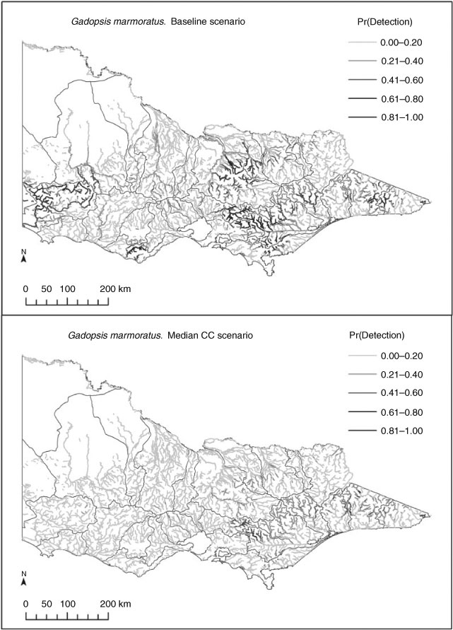
The models predicted responses by most species to each of the three climate-change scenarios, with range contractions and range expansions as well as overall range shifts (i.e. balanced contraction and expansions; Table 4) for both native and exotic species. Results differed depending on the approach to summarising range shifts. For example, some species showed consistent changes in both total occupied stream length and changes in the length of stream having high rates of occurrence (Pr > 0.5). Species showing strong and consistent range contractions included Gadopsis bispinosus and Gadopsis marmoratus, and the exotic species Salmo trutta and Oncorhynchus mykiss. Species showing predicted range expansions included Macquaria ambigua, and several diadromous and estuarine species often encountered in the lower reaches of coastal rivers, as well as several exotic species, including Gambusia holbrooki and Misgurnus anguillicaudatus. A larger group of species showed inconsistent trends, with some showing range increases overall, but substantial declines in the length of stream with high occurrence probabilities (e.g. Nannoperca variegata and Philypnodon grandiceps) or vice versa. The direction of response by such species also tended to vary with each climate scenario (Table 4). These various patterns of losses and gains from reaches with historically low, moderate and high occurrence probabilities are represented by changes in the occurrence of G. marmoratus, M. ambigua, P. grandiceps and S. trutta (Fig. 2), as are the resultant range shifts based on comparisons of historical and median climate change-predicted distribution maps (Fig. 3a–d). Confidence intervals for individual scenarios (baseline and median climate change) for these four species were also relatively narrow, as were those for relative changes in predicted occupancy under the median climate-change scenario, which ranged from ±~3% for S. trutta to approximately ±~15% for M. ambigua (Table 5).

|

|
|

|
Discussion
Predicted ‘baseline’ distributions
We developed SDMs to describe the historic distributions of 43 species of freshwater fish in Victoria, south-eastern Australia. Together with detailed response functions for influential predictor variables, the resultant maps provide a useful approach for examining predicted range shifts as well as the utility of SDMs in generating information that can be used to guide the development of mechanistic models. An important strength of BRTs is their capacity to fit non-linear response functions that more adequately describe species responses to environmental gradients than is possible with traditional modelling approaches such as linear regression. Such utility is associated with an increasing array of modelling tools (Elith et al. 2010). Importantly, our analyses suggest such non-linear associations with hydro-climatic variables are common. For example, the species for which we presented detailed analyses of environmental drivers, all showed strong threshold relationships to at least some of the predictor variables, especially temperature and the occurrence of cease-to-flow spells, a feature of the hydrologic regime that is frequently regarded as an important threshold in flowing waters (Boulton and Hancock 2006). Thus, although correlative approaches such as this cannot demonstrate causality, nor elucidate specific mechanisms (Sinclair et al. 2010), the results strongly concord with expectations derived from other independent sources of information, and could help devise quantitative and testable hypotheses.
In more general terms, the models also help provide a clear narrative describing the types of environment in which each of these species is most commonly encountered. For example, the models predict that river blackfish (G. marmoratus) occurs primarily in perennial streams with annual maximum and minimum temperatures in the range of ~8–15°C and relatively stable annual and daily flow volumes. Similarly, S. trutta mostly occupy small, perennial streams at higher altitudes (above ~200 m) with high baseflow, catchment rainfall exceeding ~1000 mm year–1, and annual average maximum temperatures not exceeding ~18°C. Reported critical thermal maxima for S. trutta range between 23.5–26.7°C, with optimal water temperatures in the range of 8–17°C (Barton 1996). Given that our data are based on average maximum air temperatures, this suggests a reasonably high level of concordance, although more accurate reconciliation of these different measures of temperature would require further work. In contrast, M. ambigua are clearly restricted to larger lowland rivers (large catchment area and baseflow volumes). Further, M. ambigua was more prevalent in regions with summer air temperatures >20°C and high inputs of solar radiation, whereas P. grandiceps appears to occupy primarily intermittent streams, including those with smaller catchments than those where M. ambigua was observed. These descriptions are derived directly from an examination of the partial plots for influential predictors (Fig. 1a–c), but (reassuringly) are largely consistent with the types of qualitative habitat descriptions in many texts (e.g. Merrick and Schmida 1984; Koehn and O’Connor 1990), but with additional quantitative support drawn from a data-driven assessment of important predictors. Occasionally, the partial plots identify inexplicable patterns, such as the sharp downward trend in occupancy for P. grandiceps at ~18°C (average annual maximum temperature). These anomalies can reflect biases in the distribution of sampling locations, with respect to environmental predictors. Our approach was to remove or modify (by making monotonic) such anomalous relationships if they had a large influence on the model predictions (note that TMAX_ANN had a very low influence, Fig. 1c), and to focus on the more influential variables for inference. An alternative approach recently advocated by Elith et al. (2010) is to simplify tree complexity during the model-building process, which has the effect of smoothing the response functions.
Predicted climate change-induced range shifts
When combined with future climate scenarios, our models predicted potentially severe impacts of climate change for some species, including potential losses of populations from entire catchments. For example, the models predicted almost a complete loss of river blackfish (G. marmoratus) from some north-flowing drainages in Victoria, an area where the species has already undergone substantial range contractions and population declines as a result of anthropogenic disturbances (Trueman 2007). The predicted contractions for this species in terms of the types of habitats affected are also consistent with observed declines in South Australia (Dale McNeil, pers. comm.) and in parts of the Loddon and Goulburn catchments in north-central Victoria during recent drought (N. Bond, unpubl. data). At the same time, however, whereas some range contractions have been consistent with recent drought impacts, the same cannot be said for range expansions, with as yet limited evidence to suggest that any of the species predicted to increase their range (such as M. ambigua and G. holbrooki) have done so, despite overall warmer (+0.8°C) and drier (–15% rainfall) conditions across Victoria over the past 10 years (Bond et al. 2008). On the one hand, such expansions may have occurred, but are yet to be documented. On the other hand, there is a suite of reasons why range expansions may not occur, or may occur more slowly than species are extirpated, including physical and biological constraints on dispersal (e.g. barriers, sedentary behaviour), and the influence of important local drivers such as physical habitat features, short-term hydrologic events, food availability or biotic interactions, which may constrain species expansions – many of the factors that have led some authors to caution on the use of SDMs in predicting range shifts (Guisan and Thuiller 2005; Sinclair et al. 2010). Our view is that predictions arising from these models are a useful step forward in framing discussions about such limitations, and hence are a useful tool in advancing our general understanding of climate-change impacts, even where the initial model predictions may be questioned – a conclusion shared by Araújo et al. (2005). This can also lead to the identification of critical knowledge and data gaps. For example, an obvious shortcoming identified in the present study for which a statistical work-around was required was the lack of spatially distributed information on both current and potential future hydrologic characteristics of rivers, a gap that reflects the difficulty in modelling hydrology at high spatial and temporal resolutions, particularly in more intermittent systems (Smakhtin 2001). This data gap is likely to continue to hamper our ability to refine predictions of ecological change in response to shifting environmental conditions in ungauged catchments.
Uncertainty in range-shift forecasts
We attempted to capture some indication of the uncertainty in the model predictions for some species, although these are expressed here only in tabular form (Table 5), and are restricted to uncertainty associated with the SDMs themselves under each of the modelled climate scenarios. Additional uncertainty in global circulation models (GCMs) and future CO2 concentrations (expressed here as different scenarios) also adds substantially to uncertainty in future predictions when expressed quantitatively alongside uncertainty in the species models (Lyons et al. 2010). Differences between our scenarios support the fact that even if species distributions can be modelled well, there is still much uncertainty in how species ranges may change because of uncertainty about how the climate will change. There is also a host of other sources of uncertainty that we have not touched on, including the extent to which SDMs can be used to extrapolate to novel climates (e.g. see Williams and Jackson 2007; Elith et al. 2010), and the way that hydrologic characteristics may change as a result of altered ground–surface water interactions under a drier climate – again something that is not captured in our efforts to model hydrology. Thus, although incorporating uncertainty in predictions based on the capacity of the models to predict historic distributions is important in demonstrating their validity, this aspect of uncertainty is just one of those that needs to be considered when extrapolating to the future (Elith and Leathwick 2009). SDMs can also be highly sensitive to species prevalence in the datasets used to derive the models, both in terms of their predictive performance (Olden et al. 2002), and also in the extent to which existing distributions (the realised niche) may influence predictions of future range (Dormann 2007). In the present study, there were several now relatively rare, but historically more common and widespread taxa for which models of the realised niche based on contemporary data probably underestimate the historical realised niche. Examples include Bidyanus bidyanus, Galaxias fuscus, Maccullochella macquariensis, Macquaria australasica and Prototroctes maraena. For the reasons discussed above, we would expect greater uncertainties in the predicted impacts of climate shifts on these rare species relative to those that are more common.
Pros and cons of using SDMs to predict range shifts
Much of the discussion of possible climate-change impacts on species distributions in Australia has been based on relatively simple qualitative assessments of existing observational and experimental data (e.g. Morrongiello et al. 2011; Booth et al. 2011). One strength of these approaches is the ability to incorporate novel aspects of species biology that may be important in determining climate-change responses, but which may be difficult to infer from SDMs because of their specific data requirements and application at large scales. At the same time, generic statements of possible impacts are also much less well suited to producing spatially explicit predictions that can feed into decisions about how to prioritise restoration and conservation programs in the face of climate change. There has been much debate about the relative merits of SDMs in predicting climate change-induced range shifts. For example, numerous authors point to the potential pitfalls associated with the exclusion of species interactions, dispersal constraints and the potential role of evolution (adaptation capacity) in determining how species will respond to climate change (e.g. Davis et al. 1998; Sinclair et al. 2010). At the same time, there is a pressing need to begin developing quantitative predictions, not least to enable the strengths and weaknesses of different modelling approaches to be evaluated – either explicitly through field validation or by comparing the results derived from qualitatively different modelling approaches (e.g. Elith et al. 2010).
Summary and conclusions
Overall, our models predicted the combined impacts of altered temperature and hydrologic regimes arising from climate change to cause marked shifts in the distribution of many freshwater fish species. Primary axes of response were shifts upward along altitudinal gradients and shifts southward (including both range expansions and contractions) in response to climate warming, and the loss of species from increasingly intermittent and ephemeral waterways, which overall were predicted to become more common. Similar climate-change impacts have been predicted in other parts of the world (e.g. Chu et al. 2005; Lyons et al. 2010). An obvious next step from a management perspective is to combine the model results for these and other species, and to apply conservation-planning approaches to identify river reaches that maximise species-occupancy patterns under both historical and potential future climate regimes. Results from such an analysis would support efforts to prioritise investment in restoration and protection strategies, and also guard against investing in reaches that may fail to support currently occurring species in the future.
Although the predictions from these models remain just that, we contend that, together with the additional information on species responses to environmental gradients, they represent an important step in gaining a more complete understanding of how climate-change impacts may play out in the long term, and an essential step in developing appropriate response strategies.
Acknowledgements
We thank John Koehn for organising the special issue and providing useful feedback on the manuscript. The work was funded by the Victorian Department of Sustainability and Environment, and Sam Marwood provided valuable guidance and project management. Mark Kennard, Bill Young, Francis Chiew, Rory Nathan John Koehn, Andrew Boulton and an anonymous reviewer variously provided valuable contributions in the form of data, and comments on the project and manuscript. Thanks also go to Darren Twiggy Giling for his efforts in bringing together the various datasets.
References
Araújo, M. B., Pearson, R. G., Thuiller, W., and Erhard, M. (2005). Validation of species–climate impact models under climate change. Global Change Biology 11, 1504–1513.| Validation of species–climate impact models under climate change.Crossref | GoogleScholarGoogle Scholar |
Balcombe, S. R., Sheldon, F., Capon, S. J., Bond, N. R., Marsh, N., Hadwen, W. L., and Bernays, S. J. (2011). Climate-change threats to native fish in degraded rivers and floodplains of the Murray–Darling Basin, Australia. Marine and Freshwater Research 62, 1099–1114.
| Climate-change threats to native fish in degraded rivers and floodplains of the Murray–Darling Basin, Australia.Crossref | GoogleScholarGoogle Scholar |
Barton, B. A. (1996). General biology of salmonids. In ‘Principles of Salmonid Culture’. (Eds W. Pennel and B. A. Barton.) pp. 29–96. (Elsevier: Amsterdam.)
Bond, N. R., Lake, P. S., and Arthington, A. H. (2008). The impacts of drought on freshwater ecosystems: an Australian perspective. Hydrobiologia 600, 3–16.
| The impacts of drought on freshwater ecosystems: an Australian perspective.Crossref | GoogleScholarGoogle Scholar |
Bond, N. R., McMaster, D., Reich, P., Thomson, J., and Lake, P. S. (2010). Modelling the impacts of flow regulation on fish distributions in naturally intermittent lowland streams: an approach for predicting restoration responses. Freshwater Biology 55, 1997–2010.
| Modelling the impacts of flow regulation on fish distributions in naturally intermittent lowland streams: an approach for predicting restoration responses.Crossref | GoogleScholarGoogle Scholar |
Booth, D. J., Bond, N., and Macreadie, P. (2011). Detecting range shifts among Australian fishes in response to climate change. Marine and Freshwater Research 62, 1027–1042.
| Detecting range shifts among Australian fishes in response to climate change.Crossref | GoogleScholarGoogle Scholar |
Boulton, A. J., and Hancock, P. J. (2006). Rivers as groundwater-dependent ecosystems: a review of degrees of dependency, riverine processes and management implications. Australian Journal of Botany 54, 133–144.
| Rivers as groundwater-dependent ecosystems: a review of degrees of dependency, riverine processes and management implications.Crossref | GoogleScholarGoogle Scholar |
Buckley, L., Urban, M., and Angilletta, M. (2010). Can mechanism inform species’ distribution models? Ecology Letters 13, 1041–1054.
Buisson, L., and Grenouillet, G. (2010). Predicting the potential impacts of climate change on stream fish assemblages. American Fisheries Society Symposium 73, 327–346.
Bureau of Meteorology (2002). ‘Climatic Atlas of Australia.’ (Bureau of Meteorology, National Climate Centre: Canberra.)
Burgman, M. A. (2005). ‘Risks and Decisions for Conservation and Environmental Management.’ (Cambridge University Press: Cambridge, UK.)
Chu, C., Mandrak, N., and Minns, C. (2005). Potential impacts of climate change on the distributions of several common and rare freshwater fishes in Canada. Diversity & Distributions 11, 299–310.
| Potential impacts of climate change on the distributions of several common and rare freshwater fishes in Canada.Crossref | GoogleScholarGoogle Scholar |
CSIRO (2008). Water availability in the Murray–Darling Basin. A report to the Australian Government from the CSIRO Murray–Darling Basin Sustainable Yields Project. Commonwealth Scientific and Industrial Research Organisation, Canberra.
Davis, A. J., Jenkinson, L. S., Lawton, J. H., Shorrocks, B., and Wood, S. (1998). Making mistakes when predicting shifts in species range in response to global warming. Nature 391, 783–786.
| Making mistakes when predicting shifts in species range in response to global warming.Crossref | GoogleScholarGoogle Scholar | 1:CAS:528:DyaK1cXhtlCjtrg%3D&md5=bbc7b8fd21cb788fbcce4a8e2c6236eeCAS |
Dormann, C. F. (2007). Promising the future? Global change projections of species distributions. Basic and Applied Ecology 8, 387–397.
| Promising the future? Global change projections of species distributions.Crossref | GoogleScholarGoogle Scholar |
Efron, B., and Tibshirani, R. J. (1997). Improvements on cross-validation: the 632+ bootstrap method. Journal of the American Statistical Association 92, 548–560.
| Improvements on cross-validation: the 632+ bootstrap method.Crossref | GoogleScholarGoogle Scholar |
Elith, J., and Leathwick, J. (2009). Species distribution models: ecological explanation and prediction across space and time. Annual Review of Ecology 40, 677–697.
Elith, J., Leathwick, J. R., and Hastie, T. (2008). A working guide to boosted regression trees. Journal of Animal Ecology 77, 802–813.
| A working guide to boosted regression trees.Crossref | GoogleScholarGoogle Scholar | 1:STN:280:DC%2BD1cvgsFOqsQ%3D%3D&md5=dae18717f2940b59ab5402e351c09a58CAS |
Elith, J., Kearney, M., and Phillips, S. (2010). The art of modelling range-shifting species. Methods in Ecology and Evolution 1, 330–342.
| The art of modelling range-shifting species.Crossref | GoogleScholarGoogle Scholar |
Friedman, J. H. (2001). Greedy function approximation: a gradient boosting machine. Annals of Statistics 29, 1189–1232.
| Greedy function approximation: a gradient boosting machine.Crossref | GoogleScholarGoogle Scholar |
Gibson, C., Meyer, J., Poff, N., Hay, L., and Georgakakos, A. (2005). Flow regime alterations under changing climate in two river basins: implications for freshwater ecosystems. River Research and Applications 21, 849–864.
| Flow regime alterations under changing climate in two river basins: implications for freshwater ecosystems.Crossref | GoogleScholarGoogle Scholar |
Growns, I., and West, G. (2008). Classification of aquatic bioregions through the use of distributional modelling of freshwater fish. Ecological Modelling 217, 79–86.
| Classification of aquatic bioregions through the use of distributional modelling of freshwater fish.Crossref | GoogleScholarGoogle Scholar |
Guisan, A., and Thuiller, W. (2005). Predicting species distribution: offering more than simple habitat models. Ecology Letters 8, 993–1009.
| Predicting species distribution: offering more than simple habitat models.Crossref | GoogleScholarGoogle Scholar |
Heikkinen, R., Luoto, M., and Araújo, M. (2006). Methods and uncertainties in bioclimatic envelope modelling under climate change. Progress in Physical Geography 30, 751–777.
| Methods and uncertainties in bioclimatic envelope modelling under climate change.Crossref | GoogleScholarGoogle Scholar |
IPCC (2001). ‘Climate Change 2001: Working Group I: The Scientific Basis.’ Contribution of Working Group I to the Third Assessment Report of the Intergovernmental Panel on Climate Change. (Eds J. T. Houghton, Y. Ding, D. J. Griggs, M. Noguer, P. J. van der Linden, X. Dai, K. Maskell and C. A. Johnson.) (Cambridge University Press: Cambridge, UK and New York, USA.)
Jones, R., and Durack, P. (2005). ‘Estimating the Impacts of Climate Change on Victoria’s Runoff Using a Hydrological Sensitivity Model.’ (CSIRO Atmospheric Research: Melbourne.)
Kearney, M., and Porter, W. (2009). Mechanistic niche modelling: combining physiological and spatial data to predict species’ ranges. Ecology Letters 12, 334–350.
| Mechanistic niche modelling: combining physiological and spatial data to predict species’ ranges.Crossref | GoogleScholarGoogle Scholar |
Kennard, M. J., Olden, J. D., Arthington, A. H., Pusey, B. J., and Poff, N. L. (2007). Multiscale effects of flow regime and habitat and their interaction on fish assemblage structure in eastern Australia. Canadian Journal of Fisheries and Aquatic Sciences 64, 1346–1359.
| Multiscale effects of flow regime and habitat and their interaction on fish assemblage structure in eastern Australia.Crossref | GoogleScholarGoogle Scholar |
Kennard, M. J., Mackay, S. J., Pusey, B. J., Olden, J. D., and Marsh, N. (2010a). Quantifying uncertainty in estimation of hydrologic metrics for ecohydrological studies. River Research and Applications 26, 137–156.
Kennard, M. J., Pusey, B. J., Olden, J. D., Mackay, S. J., Stein, J. L., and Marsh, N. (2010b). Classification of natural flow regimes in Australia to support environmental flow management. Freshwater Biology 55, 171–193.
| Classification of natural flow regimes in Australia to support environmental flow management.Crossref | GoogleScholarGoogle Scholar |
Koehn, J. D., and O’Connor, W. G. (1990). ‘Biological Information for Management of Native Freshwater Fish in Victoria.’ (Department of Conservation and Environment: Melbourne.)
Leathwick, J. R., Rowe, D., Richardson, J., Elith, J., and Hastie, T. (2005). Using multivariate adaptive regression splines to predict the distributions of New Zealand’s freshwater diadromous fish. Freshwater Biology 50, 2034–2052.
| Using multivariate adaptive regression splines to predict the distributions of New Zealand’s freshwater diadromous fish.Crossref | GoogleScholarGoogle Scholar |
Lyons, J., Stewart, J. S., and Mitro, M. (2010). Predicted effects of climate warming on the distribution of 50 stream fishes in Wisconsin, USA. Journal of Fish Biology 77, 1867–1898.
| Predicted effects of climate warming on the distribution of 50 stream fishes in Wisconsin, USA.Crossref | GoogleScholarGoogle Scholar | 1:STN:280:DC%2BC3cbnt1SmtQ%3D%3D&md5=b9c400978e0c89ba95a6798b9e16eeb1CAS |
Morrongiello, J. R., Beatty, S. J., Bennett, J. C., Crook, D. C., Ikedife, D. N. E. N., Kennard, M. J., Kerezsy, A., Lintermans, M., McNeil, D. G., Pusey, B. J., and Rayner, J. (2011). Climate change and its implications for Australia's freshwater fish. Marine and Freshwater Research 62, 1082–1098.
| Climate change and its implications for Australia's freshwater fish.Crossref | GoogleScholarGoogle Scholar |
Merrick, J. R., and Schmida, G. E. (1984). ‘Australian Freshwater Fishes: Biology and Management.’ (Griffin Press: Netley, SA.)
Olden, J. D., Jackson, D. A., and Peres-Neto, P. R. (2002). Predictive models of fish species distributions: a note on proper validation and chance predictions. Transactions of the American Fisheries Society 131, 329–336.
| Predictive models of fish species distributions: a note on proper validation and chance predictions.Crossref | GoogleScholarGoogle Scholar |
Olden, J. D., Lawler, J. J., and Poff, N. L. (2008). Machine learning methods without tears: a primer for ecologists. The Quarterly Review of Biology 83, 171–193.
| Machine learning methods without tears: a primer for ecologists.Crossref | GoogleScholarGoogle Scholar |
Palmer, M. A., Reidy, C., Nilsson, C., Florke, M., Alcamo, J., Lake, P. S., and Bond, N. R. (2007). Climate change and the world’s river basins: anticipating response options. Frontiers in Ecology and the Environment 6, 81–89.
| Climate change and the world’s river basins: anticipating response options.Crossref | GoogleScholarGoogle Scholar |
Pearce, J., and Ferrier, S. (2000). Evaluating the predictive performance of habitat models developed using logistic regression. Ecological Modelling 133, 225–245.
| Evaluating the predictive performance of habitat models developed using logistic regression.Crossref | GoogleScholarGoogle Scholar |
Poff, N. L., and Allan, D. J. (1995). Functional organization of stream fish assemblages in relation to hydrological variability. Ecology 76, 606–627.
| Functional organization of stream fish assemblages in relation to hydrological variability.Crossref | GoogleScholarGoogle Scholar |
Poff, N. L., Tokar, S., and Johnson, P. (1996). Stream hydrological and ecological responses to climate change assessed with an artificial neural network. Limnology and Oceanography 41, 857–863.
| Stream hydrological and ecological responses to climate change assessed with an artificial neural network.Crossref | GoogleScholarGoogle Scholar |
Pollino, C. A., Feehan, P., Grace, M. R., and Harr, B. T. (2004). Fish communities and habitat changes in the highly modified Goulburn Catchment, Victoria, Australia. Marine and Freshwater Research 55, 769–780.
| Fish communities and habitat changes in the highly modified Goulburn Catchment, Victoria, Australia.Crossref | GoogleScholarGoogle Scholar |
Pratchett, M. S., Bay, L. K., Gehrke, P. C., Koehn, J. D., Osborne, K., Pressey, R. L., Sweatman, H. P. A., and Wachenfeld, D. (2011). Contribution of climate change to degradation and loss of critical fish habitats in Australian marine and freshwater environments. Marine and Freshwater Research 62, 1062–1081.
| Contribution of climate change to degradation and loss of critical fish habitats in Australian marine and freshwater environments.Crossref | GoogleScholarGoogle Scholar |
Quist, M. C., Hubert, W. A., and Rahel, F. J. (2005). Fish assemblage structure following impoundment of a Great Plains river. Western North American Naturalist 65, 53–63.
R Development Core Team (2009). ‘R: A Language and Environment for Statistical Computing.’ (R Foundation for Statistical Computing: Vienna.) Available at http://www.r-project.org/ [Accessed 3 August 2011].
Ridgeway, G. (2007). ‘Generalized Boosted Models: A Guide to the gbm Package.’ Available at http://cran.r-project.org/web/packages/gbm/gbm.pdf [accessed 5 July 2011].
Sanborn, S., and Bledsoe, B. (2006). Predicting streamflow regime metrics for ungauged streams in Colorado, Washington, and Oregon. Journal of Hydrology 325, 241–261.
| Predicting streamflow regime metrics for ungauged streams in Colorado, Washington, and Oregon.Crossref | GoogleScholarGoogle Scholar |
Sinclair, S., White, M., and Newell, G. (2010). How useful are species distribution models for managing biodiversity under future climates? Ecology and Society 15, Article 8.
Sinclair Knight Merz (2005). Development and application of a flow stresses ranking procedure. A report produced by Sinclair Knight Merz for the Department of Sustainability and Environment, Victoria, Melbourne.
Smakhtin, V. U. (2001). Low flow hydrology: a review. Journal of Hydrology 240, 147–186.
| Low flow hydrology: a review.Crossref | GoogleScholarGoogle Scholar |
Stein, J. L., Stein, J. A., and Nix, H. A. (2002). Spatial analysis of anthropogenic river disturbance at regional and continental scales: identifying the wild rivers of Australia. Landscape and Urban Planning 60, 1–25.
Stein, J. L. (2006). ‘A Continental Landscape Framework for Systematic Conservation Planning for Australian Rivers and Streams.’ (PhD Thesis, Centre for Resource and Environmental Studies, Australian National University: Canberra.) Available at http://hdl.handle.net/1885/49406 [accessed 30 August 2011].
Thuiller, W. (2007). Biodiversity: climate change and the ecologist. Nature 448, 550–552.
| Biodiversity: climate change and the ecologist.Crossref | GoogleScholarGoogle Scholar | 1:CAS:528:DC%2BD2sXosVSrsbc%3D&md5=1b487d85984d4892a37a3e4fb4c67123CAS |
Trueman, W. T. (2007). Some recollections of native fish in the Murray–Darling system with special reference to the trout cod. Native Fish Australia, Melbourne.
Walsh, C., Stewardson, M., Stein, J., and Wealands, S. (2007). ‘Sustainable Rivers Audit Filters Project Stage 2, Report to Murray Darling Basin Commission.’ (School of Enterprise, The University of Melbourne: Melbourne).
Williams, J. W., and Jackson, S. T. (2007). Novel climates, no-analog communities, and ecological surprises. Frontiers in Ecology and the Environment 5, 475–482.
| Novel climates, no-analog communities, and ecological surprises.Crossref | GoogleScholarGoogle Scholar |