Modelling long-term fire regimes of southern California shrublands

The fire regime of a landscape integrates the spatiotemporal pattern of ignitions, fuels, weather and topography, and describes the size, spatial pattern and return interval of fires (Davis and Michaelsen 1995). The current fire regime of southern California shrublands extends over a broad range of fire sizes from numerous small fires to relatively few large, intense, stand-replacing fires, at a 20- to >100-year recurrence interval (Davis and Michaelsen 1995; Moritz 1997; Keeley 2000; Moritz et al. 2005). Past fire regimes in chaparral may have been quite similar, with total area burned also dominated by large fires (Mensing et al. 1999; Keeley and Fotheringham 2003). This distribution of fire sizes is common to other fire-prone ecosystems as well (Moritz et al. 2005).

Fire regimes are dynamic, varying in response to changes in ignition frequency, vegetation and climate. In the future, climate change will likely have an effect on fuel quality and amount (Field et al. 1999; Keeley and Fotheringham 2003), whereas increases in population in the wildland–urban interface (WUI) will likely lead to increased numbers of ignitions and changes in ignition locales (Syphard et al. 2007; Moritz and Stephens 2008). A quantitative understanding of fire regime drivers will aid in understanding future fire regimes resulting from climate change and the expansion of the WUI.

In this paper, we evaluate the sensitivity of three fire regime characteristics (size distributions, maps of fire return intervals (FRIs), and cumulative total area burned) to the number and spatial pattern of ignitions; the frequency of extreme, Santa Ana wind conditions; and live fuel moisture (LFM) using HFire, a landscape fire succession model (LFSM). HFire uses a mechanistic approach to modelling fire spread, using the full Rothermel (1972) equations. It is capable of modelling both individual fires and long-term fire regimes in southern California chaparral shrubland landscapes (Peterson et al. 2009). The predictions of fire perimeters in HFire have been validated in baseline comparisons with FARSITE (Finney 1998) and hourly progressions of individual, southern California fires (Peterson et al. 2009). Modelled fire size distributions from the initial version of HFire have been shown to agree with fire size distributions for the Los Padres National Forest fire data between 1911 and 1995 (Moritz et al. 2005).

The southern California shrubland fire regime and HFire together provide a unique evaluation study for comparing actual data with model results over broad spatial and temporal scales. The relatively short southern California FRI provides an extended historical record of observations, and the computational efficiency of HFire enables quantitative evaluation of which physical parameters (ignitions, wind, LFM) are most important for determining the fire regime.

Fire modelling is a viable approach for increasing our knowledge of fire regime dynamics under a suite of conditions (Davis and Michaelsen 1995; Franklin et al. 2001; Keeley and Fotheringham 2003; Keane et al. 2004; Cary et al. 2006). Long-term simulation of fire and vegetation response has been used to examine variation in existing landscape patterns (Venevsky et al. 2002), fire effects on vegetation dynamics (Haydon et al. 2000; Franklin et al. 2001), and scenarios of management activities (Haydon et al. 2000; Miller and Urban 2000) and climate change (Davis and Michaelsen 1995; Cary and Banks 1999).

Keane et al. (2004) categorised the 44 most well-known LFSMs based on their approach to modelling four main processes: (1) vegetation succession, (2) fire ignition, (3) fire spread, and (4) fire effects. They found that for three of the processes, the models varied in degrees of stochasticity, complexity and mechanism. However, a majority (36) of the models used a simple probabilistic approach to modelling fire spread or final fire perimeters. Only eight of the models used a mechanistic approach (Rothermel 1972; Finney 1998) to simulate fire spread in an incrementally expanding manner.

Historically, mechanistic fire spread models have been considered too complex, computer-intensive and the data requirements too vast for use in long-term fire regime simulations (Hargrove et al. 2000; Venevsky et al. 2002), though their use would be preferable to empirical or stochastic approaches if they could be implemented (Keane and Finney 2003). Of the eight mechanistic models in the Keane et al. (2004) study, only Cary and Banks (1999) and Perera et al. (2008) simulated fire spread at hourly time steps with the same rigour as single-event fire spread models (e.g. Finney 1998). Cary and Banks (1999) use equations and inputs designed to simulate fire in Australian fuels, and Perera et al. (2008) use equations and inputs designed for fire simulation in Canadian boreal forest, complementing our study of southern California shrublands. Additionally, Keane et al. (1996) incorporated FARSITE (Finney 1998) fire spread simulations into their FIRE-BGC model, though they only simulated the spread of two fires within the 200-year simulation time frame, owing to the inherent low fire return interval of their fire regime. The remaining five models used simplified fire spread equations of unspecified accuracy.

HFire is a spatially explicit, raster-based model of fire growth that incorporates the Rothermel equations (Rothermel 1972, 1983) for fire spread. The Rothermel equations were developed through burning small test fires in idealised dead fuels; from these experiments, equations were developed to predict fire spread based on weather, topography, and both live and dead fuel amounts and properties. The Rothermel equations are frequently implemented in fire spread models for use in intermediate spatial and temporal resolution fire spread simulations, such as FARSITE (Finney 1998), which is operationally used by the US National Park Service and the US Forest Service in both live and dead fuels (Pastor et al. 2003). Additionally, numerous authors have utilised fire models that use the Rothermel equations to model landscapes including live fuels, finding predictions of fire spread to be reasonable (e.g. Davis and Burrows 1994; Arca et al. 2007; Dasgupta et al. 2007; Peterson et al. 2009), especially when appropriate custom fuel models (Weise and Regelbrugge 1997; Arca et al. 2007; Peterson et al. 2009) are used.

HFire can be used to simulate individual fires or long-term fire regimes (Peterson et al. 2009). The computational efficiencies built into HFire allowed us to perform 1440 fire regime simulations, each 1200 years long, for a 100 000-ha shrubland landscape in southern California. HFire code can be found at the website of the model (http://firecenter.berkeley.edu/hfire/, accessed 7 January 2011). Inputs necessary for modelling an individual event in HFire are nearly identical to those for the widely used FARSITE fire spread simulator (Finney 1998): ignition location(s); temporally varying inputs such as wind speed and direction, and live and dead fuel moistures; and digital maps of topography and fuel type. One-dimensional predictions from the Rothermel (1972) equations are fitted to two dimensions, using the solution to the ‘fire containment problem’ (Albini and Chase 1980) and the empirical double-ellipse formulation of Anderson (1983). The raster implementation utilised by HFire does not produce fractal or unrealistic fire perimeters as earlier raster models did. This is demonstrated through a series of simulations comparing FARSITE and HFire fire perimeters on both simplified and actual landscapes (Peterson et al. 2009). HFire uses an adaptive time step, allows fire to spread into a cell from all neighbouring cells over multiple time steps, and is computationally efficient – a crucial advantage in long-term simulation studies like those presented here (Peterson et al. 2009).

When HFire is used to simulate fire regimes, it implements the same fire spread algorithm and landscape inputs as in individual-event mode, with additional variables accounting for stochastic ignitions, stochastic weather variables, stochastic LFM trend, and vegetation growth and succession. It runs at an hourly time step between fires and at sub-minute intervals during fires, for hundreds to thousands of simulated years.

Fires cannot occur without ignitions. The average number of ignitions per year and the spatial distribution of ignitions are user-specified in HFire. Ignition probabilities can be spatially homogeneous or based on landscape features, such as the distance to the nearest road for fire regimes where anthropogenic ignitions are prevalent, or elevation for fire regimes where lightning strikes are the primary source of ignitions (Keeley and Fotheringham 2003). The actual number and location of these ignitions each year are then stochastically generated during the simulation runs. Ignitions that do not result in a spreading fire are identified with a size threshold parameter, and are not included in fire size statistics.

Weather is considered to be the most important variable for predicting how a fire will spread for many ecosystems, including California chaparral (Davis and Michaelsen 1995; Moritz 1997). HFire uses hourly weather data (wind speed and direction, 10-h dead fuel moisture) to model fire spread. The 10-h dead fuel moisture is commonly used to estimate 1-h and 100-h dead fuel moisture because 10-h data are measured at weather stations (Burgan et al. 1998). Weather data files are populated with historical data from weather stations within the study area. A majority of the total area burned in southern California occurs under extreme wind conditions, locally known as Santa Ana wind conditions (Countryman 1974), so HFire was designed to accommodate separate ‘standard’ and ‘extreme’ hourly weather inputs. The user specifies the annual average number and duration of extreme fire weather events per year, with the timing and actual number of extreme events per year stochastically determined by HFire. The weather values used at any given hour during the simulation period are randomly selected from the standard or extreme data files.

Live fuel moisture varies predictably on an intra-annual basis; however, it is highly variable on an interannual basis owing to differences in annual precipitation (Countryman and Dean 1979; Peterson et al. 2008). For fire regime simulations, woody and herbaceous LFM values are stochastically simulated, given annual average values and standard deviations, and seasonal trends. LFM data are available at 2-week intervals from government agencies for many regions; LFM can also be predicted using satellite data (Peterson et al. 2008).

Post-fire vegetation progresses through a series of fuel classes, represented by standard and custom fuel models (Albini 1976; Weise and Regelbrugge 1997), until it burns again. A climax, potential natural vegetation (PNV) type map is used to assign a particular successional trajectory to each pixel. Using pixel ages and regeneration trajectories, a fuel model map is produced. As the simulation progresses, age is incremented annually, or set to zero if the pixel burns, and the per-pixel fuel models change accordingly. More detail on parameterising ignitions, weather and vegetation regrowth is provided in the Methods section.

Fires go out naturally when they encounter conditions that slow them to the point of extinction (e.g. moist or sparse vegetation), or they may be actively suppressed. Fire propagation in a given HFire cell is stopped when the rate of spread drops below an extinction rate of spread (ERS) threshold. After preliminary runs of HFire, we chose a baseline ERS threshold of 0.05 m s^–1. This estimate is based on discussions with various Forest Service personnel, other fire simulation work in southern California chaparral shrublands (e.g. Davis and Burrows 1994), and comparison of preliminary model output (e.g. fire sizes, shapes, frequencies) with mapped fire history for the Santa Monica Mountains (SMM). Other LFSMs have used a similar technique to extinguish fires, basing the threshold on intensity (Cary and Banks 1999; Miller and Urban 2000) or dead fuel moisture content (Perera et al. 2008) as opposed to rate of spread.

HFire model accuracy and sensitivity have been evaluated in single-event mode by comparing observed and predicted fire spread during historical events (Peterson et al. 2009) and for simulated landscapes (Clark et al. 2008; Peterson et al. 2009). HFire has also been utilised previously in a comparison of empirical fire data, modelled fire regimes, and highly optimised tolerance (HOT) as the mechanism for ecosystem structure in fire-prone areas (Moritz et al. 2005).

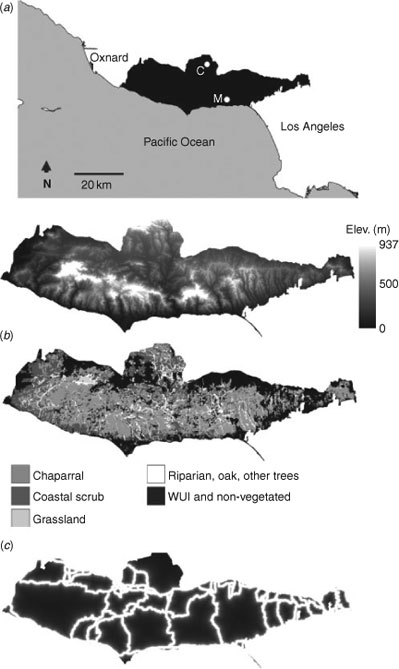
The simulation domain for this project was a 96 000-ha region encompassing the SMM National Recreation Area, abutting the Pacific Ocean and the densely populated Los Angeles metropolitan area in southern California (Fig. 1). The study area has a Mediterranean-type climate characterised by hot, dry summers and cool, wet winters. Average annual precipitation ranges from 400 mm at the coast to 600 mm at the mountain crest (Radtke et al. 1982), and exhibits a high degree of both intra- and interannual variability (Keeley 2000; National Park Service 2005). Topography is rugged, with mountain peaks over 500 m in height just a few kilometres inland from sea level (Fig. 1a). SMM is dominated by sclerophyllous, fire-dependent chaparral and drought-deciduous coastal scrub shrublands, although there are also riparian corridors, patches of invasive annual grasses, and vegetation typical of the local WUI (e.g. mixed native and non-native landscaping) (Radtke et al. 1982; National Park Service 2005).

Fig. 1.  Study area. The inset at top shows the location of the SMM (Santa Monica Mountains) study area along the coast of southern California. Points C and M indicate the locations of Cheeseboro and Malibu weather stations from which hourly weather data were obtained. Panel A demonstrates the patterns of topography in the study area. Panel B indicates aggregated vegetation class patterns in SMM (see Table 1 for detailed breakdown). Panel C indicates the road network and associated probabilities of ignition.

Fires in southern California shrublands tend to be stand-replacing; all aboveground vegetation is killed (Keeley 2000). Herbaceous vegetation is dominant the first year after the fire, with shrubs again becoming dominant 3 to 5 years after the fire (Horton and Kraebel 1955; Keeley 2000). Shrub recovery comes from basal resprouting, seedling recruitment from the prefire seed bank, or both (Keeley 2000).

Spatial fuels data for the entire SMM area were derived from a 100 × 100-m (1-ha) resolution regional PNV map (Franklin 1997), which represents the vegetation community, and therefore fuel type, that would occur in the long absence of fire. The PNV map was modified using SMM maps of riparian areas and local planning-agency maps of recent housing development. Vegetation communities of the PNV map (Fig. 1b) capable of carrying wildfire during typical weather conditions were then crosswalked to 1 of the 13 standard fuel models (Albini 1976) or to custom fuel models for southern California shrubland vegetation (Weise and Regelbrugge 1997). Vegetation types and their associated fuel models are shown in Table 1, and details of the fuel models are summarised in Table A1 of the Accessory publication (available from the journal online, see http://www.publish.csiro.au/?act=view_file&file_id=WF09102_AC.pdf).

Table 1.  Vegetation, regrowth characteristics and associated fuel models
These classes represent the mapped PNV (potential natural vegetation) types within the study area and their simplified paths of fuel regrowth after a fire. For classes that are assumed to accumulate biomass with age, fuel models change with time since fire, and the relevant time periods for each stage are given in parentheses. Both standard (Northern Forest Fire Laboratory, NFFL (Albini 1976)) and custom fuel model parameter estimates are provided in Table A1 of the Accessory publication (http://www.publish.csiro.au/?act=view_file&file_id=WF09102_AC.pdf). NPS, National Park Service; WUI, wildland–urban interface

The progression of fuels after a fire depends on the local PNV type. Some types regenerate on an annual basis, such as grass-dominated areas (National Park Service 2005), and others remain relatively constant (e.g. WUI type). Most vegetation, however, is allowed to develop towards its late-successional PNV type, being progressively assigned fuel models that reflect accumulating biomass and larger stem diameters (Table A1). The initial fuel model map was generated using the initial stand age (from fire history of SMM as of 1999) and PNV maps.

Long-term fire regime sensitivity to the following four variables was evaluated: the number of ignitions per year, the spatial pattern of ignitions, the number of Santa Ana events per year, and LFM trend. Baseline settings for these variables are discussed below. HFire was run at 1-ha pixel resolution for fuels and other spatial inputs, leading to an 870 × 300-pixel modelling domain. Simulations were 1200 years long, but the first 200 years of each run were discarded to address possible sensitivities to initial conditions, leaving 1000 years of simulated fires for analysis. Fire spread was modelled for the period from 1 July to 30 November each year, the period of high fire risk for southern California (National Park Service 2005). In fact, 70% of the historical fires recorded in SMM, and 83% of the area burned, occurred between 1 July and 30 November (R. Taylor, pers. comm.).

The mapped fire history for SMM is incomplete in the early 1900s (R. Taylor, pers. comm.), so it was not possible to estimate reliable annual average ignition frequencies from this dataset. The southern portion of the Los Padres National Forest (LPNF), however, is a nearby shrubland-dominated region with a relatively complete ignition and fire perimeter record (Moritz 1999), providing rough estimates of ignition frequencies per unit area. On average, shrublands of LPNF experienced a total of 0.37 ignitions per square kilometre over the period 1911–95. Therefore, for a region the size of SMM (960 km²), a baseline estimate of 4.0 ignitions per year was chosen. Other values tested in the model runs were 1.0, 8.0 and 12.0 ignitions per year. Most ignitions are not likely to propagate and become fires in reality, as they are extinguished by human activity quickly or they go out before successfully igniting fuels that will promote further spread (Perera et al. 2008). This is incorporated into the model with a failed ignition size parameter, which was set to one pixel (i.e. fires must progress out of the initial pixel to be counted).

In addition, HFire allows the user to specify ignition location probabilities, for example increased probabilities along roads (Fig. 1c). In the SMM, 155 of the 161 fires from 1981 to 2003 were anthropogenic in origin, the remaining six were due to lightning strikes (National Park Service 2005), and anthropogenic ignitions have been shown to preferentially occur close to roads (Keeley and Fotheringham 2003; Syphard et al. 2008). We tested (i) spatially homogeneous and (ii) spatially correlated ignition probabilities. For the latter case, we used a piece-wise linear function whereby relative ignition probability was uniform at 1.0 up to 100 m from a road bed, and decreased to 0.1 at 1000 m from the road bed.

Fire weather conditions can have a very strong influence on fire regimes, and this is especially true for chaparral-dominated shrublands (Davis and Michaelsen 1995; Moritz 1997; Keeley and Fotheringham 2003). We separated fire weather data from 1997 to 2007 from two weather stations in SMM (Cheeseboro and Malibu) into either ‘standard’ or ‘extreme’ days, by examining relative humidity, wind speed and wind azimuth data, and a list of Santa Ana days determined by Raphael (2003). This resulted in 3000 days of hourly observations for standard weather. The extreme fire weather dataset is 10% of this size, consisting of 276 days of hourly observations. A polar plot was used to show wind speed and azimuth values for the standard and extreme datasets (Fig. 2). Standard winds can blow from any direction, with south-west winds (wind blowing from the south-west) generally having the highest wind speeds. Extreme winds, with high wind speeds, generally blow from ~20° to 95°. The lower wind speeds in the extreme dataset are due to: (1) lulls in the winds mid-event and (2) HFire requires the classification of weather data as standard or extreme on a daily basis rather than an hourly one, thus incorporating standard weather conditions at the beginning and end of extreme events.

Fig. 2.  Polar plot showing historical (1997–2007) wind speed (miles per hour) and direction data under normal (black) and Santa Ana (red) conditions for the Cheeseboro and Malibu weather station, SMM (Santa Monica Mountains).

The weather data stream used in the model switches from standard to extreme weather a user-specified number of times, corresponding to the average number of Santa Ana events per fire year, for a user-specified length of time. The 1997–2007 average Santa Ana frequency was 5.2 events, with a standard deviation of 1.2 within the 1 July–30 November HFire simulation period. Values tested in the model runs were averages of 0.0, 1.0, 2.0, 4.0, 8.0 and 16.0 Santa Ana events per year. The average duration of an event was calculated from the 1997–2007 weather data to be 2.4 days.

Live fuel moisture, a measure of the water content of live vegetation, affects rate of spread and ignition success (Countryman and Dean 1979). LFM is particularly important in the shrublands of southern California as a large proportion (55–75%) of the biomass available to fires is living, so fires will only propagate if LFM is low (Countryman and Dean 1979; Dennison et al. 2008). Dennison et al. (2008) examined the fire history of the SMM and found that all large fires occurred at an LFM below 77%. LFM is input into HFire separately for woody and for herbaceous fuels (Fig. 3). We used average values for Los Angeles County chaparral for woody LFM and Los Angeles County coastal sage scrub (CSS) for herbaceous LFM. The data were provided by the Los Angeles County Fire Department. LFM follows a sinusoidal trend annually, with maximum values in early spring and minima in the fall. Three different LFM trends were tested: the average trend (1982–2007) during (i) wet years, and (ii) dry years, and (iii) a temporally invariant trend (60% for woody fuels, 105% for herbaceous fuels) that might be used if more detailed information was unavailable. It can be seen that the peak LFM for CSS is nearly double that of chaparral, and that it occurs earlier in the year, owing to CSS species having shallower roots. The differences between the two are lessened during the HFire simulation period of 1 July–30 November (Fig. 3). The average standard deviations during the simulation period (wet; dry) were (10.0; 5.2) for woody LFM, (40.0; 27.0) for herbaceous LFM, and (5.0; 5.0) for the temporally invariant trend.

Fig. 3.  Live fuel moisture trends (LFM) used in the HFire model runs; data derived from the Los Angeles County Fire Department LFM monitoring program.

We examined three aspects of fire regimes: fire size distributions, FRI maps, and cumulative total area burned. Sensitivity to two categorical and two continuous independent variables was assessed: spatial ignition pattern (uniform, increased number of ignitions closer to roads), live fuel moisture trend (wet, dry, constant value), ignition frequency (1.0, 4.0, 8.0, 12.0 per year), and Santa Ana event frequency (0.0, 1.0, 2.0, 4.0, 8.0, 16.0 per year). Ten replicates of each scenario were performed, varying the starting random number seed, in order to make the results more robust. Hence, a total of 1440 (2 ignition pattern ×3 LFM × 4 ignition frequency × 6 Santa Ana frequency ×10 replicates) 1200-year model runs were performed.

Analysis of covariance (ANCOVA) was performed on the total area burned, which was transformed using the natural logarithm to make the data follow a normal distribution, similarly to Cary et al. (2006). Linear regression is used to test relationships between a continuous dependent variable and continuous independent variables, analysis of variance (ANOVA) is used to test relationships between a continuous dependent variable and categorical independent variables, and ANCOVA allows for both continuous and categorical variables to be tested in the same model. Tukey’s honestly significantly different (HSD) post-hoc pairwise comparisons are used to determine which levels of a categorical variable are significantly different once ANOVA determines that the variable is significant. Statistical analysis was performed within the R free software environment (R Development Core Team 2008).

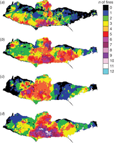
Reasonable, baseline parameter settings (uniform ignitions, 4.0 ignitions per year, 4.0 Santa Ana events per year, wet LFM) simulated a fire regime that is representative of general fire patterns in SMM (Fig. 4). In the SMM 1910–2007 fire history, the highest fire frequency occurs at the southern boundary (the mountain range adjacent to the Pacific Ocean), with the central southern portion having the most fires. There is another region of high fire frequency in the north central portion. Much of the east portion experienced zero to one fires in the period 1910–2007. Fig. 4 also shows the last 100 years of modelled fire history for three of ten randomly selected HFire baseline parameter runs. Patterns in the simulated fire histories are also present in the actual fire history. All three model results show a greater number of fires in the southern part of the area, two of the three show enhanced fire frequency in the north central region, and fire frequency is reduced in the eastern portion of SMM.

Fig. 4.  Fire frequency for SMM (Santa Monica Mountains), actual 1910–2007 (a), and the last 100 years of three randomly selected HFire runs (b–d) using baseline parameters (aspatial ignitions, four ignitions per year, four Santa Ana events per year, wet LFM (live fuel moisture)).

A commonly used fire regime metric is the FRI, defined to be the average number of years between fires. The average FRI of the 10 random baseline runs was 37.2 years for the wet LFM trend and 21.4 years for the dry LFM trend (Table 2). These values envelop the published value of 32 years for SMM, which experienced a mixture of wet and dry years in the 1910–2007 period (National Park Service 2005).

Table 2.  Fire regime metrics for baseline parameter settings of HFire (aspatial ignitions, four ignitions per year, four Santa Ana events per year, wet live fuel moisture (LFM))
Values for constant and dry LFM are also shown. Columns 2–7 indicate the following: number of actual ignitions simulated over the period analysed; percentage of ignitions becoming fires; fire return interval, median fire size, mean fire size, and coefficient of variation (CV) in fire size

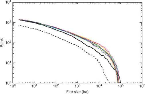
Plots of simulated (1000 years) and actual fire size distributions demonstrate that the baseline parameter settings generated distributions that are similar in form to that of the chaparral-dominated portions of LPNF (Fig. 5), indicating that simulated fire regimes approximate those observed in real shrubland ecosystems well. The distributions of fire sizes follow a power law, characterised by many very small events extending broadly out to relatively few larger events (Fig. 5; Moritz 1997; Moritz et al. 2005; Cui and Perera 2008). The LPNF shrubland dataset represents a largely complete fire history that includes even very small events (Moritz 1999). The data were originally compiled in 1997, and have been updated through 2007 by including fires recorded by CAL FIRE (Moritz 1999; FRAP 2009). LPNF is 10 times larger than SMM, but the fire record (1910–2007) is ~1/10th as long as the HFire simulation period, so the number of fires recorded was comparable. The SMM fire history (R. Taylor, pers. comm.) is also included on the plot (Fig. 5), showing the form of both historical chaparral datasets is similar, despite the smaller number of fires and reduced large fire size due to the reduced size of the study area.

Fig. 5.  Historical LPNF (Los Padres National Forest) (black) and historical SMM (Santa Monica Mountains) (dashed black) v. simulated (10 coloured lines) HFire baseline parameterisation fire size distributions. The historical LPNF dataset includes all chaparral fires in LPNF from 1911 to 1995 plus CAL FIRE data from 1996 to 2007. The historical SMM dataset covers 1910–2008 and contains all known fires. The historical datasets were subset to only include fires larger than 2 ha, the minimum fire size generated by HFire. The data were sorted by fire size in descending order (largest fire has a rank of 1).

The large difference between median and mean fire sizes shown in Table 2 is also consistent with a power-law fire size distribution. Other measures characterising the simulated baseline fire regime, such as the percentage of ignitions propagating to become fires and the coefficient of variation (CV) in fire size, are also given in Table 2.

This section examines changes in fire size distributions and maps of FRIs resulting from varying ignition pattern and frequency, Santa Ana frequency and LFM trend, as well as univariate relationships between those independent variables and the natural logarithm of total burned area. Linear regression results are provided for the continuous variables and ANOVA results are provided for the categorical variables.

Fig. 6 shows the effect of varying the four independent variables on fire size distributions. The distributions shown represent the sum of all of the fires from the 10 HFire runs having a different random number seed. Baseline settings (uniform ignitions, 4.0 ignitions per year, 4.0 Santa Ana events per year, wet LFM) were used for the variables that were held constant in the simulations. Varying the number of Santa Ana events has minimal effect on the total number of fires, and the size of the 10 largest fires; however, the distribution of medium to large fire sizes is very different (Fig. 6a). The size of the 1000th fire increases from ~2000 ha for the 0.0 Santa Ana cases to 30 000 ha for the 16.0 Santa Anas per year cases. Many more medium to large fires occur under more extreme weather conditions. Varying the number of ignitions has a different effect. As the number of ignitions per year increases, the number of fires increases (Fig. 6b). However, the fire size distribution lines cross in the figure, and the 12.0 ignitions per year case has the lowest largest fire size, as previously burned areas within the same fire season act as fire breaks for subsequent fires. The variability in fire size distributions is lower for the remaining two variables. Dry LFM generally leads to larger fires, although the largest fires within the 1000 year modelling period are of similar size for the wet LFM case (Fig. 6c). Having no set ignition pattern led to slightly larger intermediate fire sizes, but the largest fires were of the same size (Fig. 6d).

Fig. 6.  Cumulative fire-size probability distributions, summing the 10 different random runs varying (a) the number of Santa Ana events per year (0, 1, 2, 4, 8, 16; red, green, blue, cyan, magenta, black); (b) the number of ignitions (1, 4, 8, 12; black, red, green, blue); (c) the live fuel moisture (constant, wet, dry; black, red, green); and (d) the ignition pattern (no pattern, higher probability closer to roads; black, red). The data were sorted by fire size in descending order (largest fire has a rank of 1).

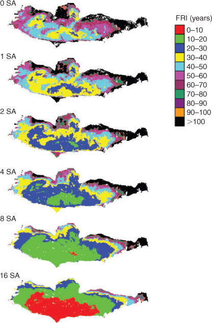
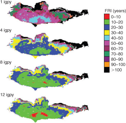
The FRI maps show that spatial variability in FRI is high for all four independent variables (Figs 7–9). The FRI maps presented here were constructed by averaging the FRI maps from the 10 differently seeded HFire runs. Areas in red on the maps experience FRI less than 10 years, making them susceptible to type-conversion (Keeley et al. 2005). Fig. 7 shows the effect of varying the number of Santa Ana events. As with Fig. 4a, which showed the fire history of the past 100 years, Fig. 7 shows that the eastern and northerly western portions of the SMM burn less regularly. The FRI decreases with increasing numbers of Santa Ana events, with only the far eastern portion showing values greater than 100 years for the 16.0 Santa Ana events case. This is to be expected as winds blow from the north-east during Santa Anas, and fires do not readily spread upwind.

Fig. 7.  Fire return interval maps for 1000 years of fires for SMM (Santa Monica Mountains), showing the effect of increasing the number of Santa Ana (SA) events from 0 to 16 per year. Other parameters held constant were four ignitions per year, wet LFM (live fuel moisture), and uniform ignition probabilities.

Fig. 8.  Fire return interval maps for 1000 years of fires for SMM (Santa Monica Mountains), showing the effect of increasing the number of ignitions per year (igpy) from 1 to 12. Other parameters held constant were four Santa Ana events per year, wet LFM (live fuel moisture), and uniform ignition probabilities.

Fig. 9.  Fire return interval maps for 1000 years of fires for SMM (Santa Monica Mountains), showing the effect of changing LFM (live fuel moisture) from constant (a), to average dry trend (b), to average wet trend (c). Other parameters held constant were four Santa Ana events per year, four ignitions per year, and uniform ignition probabilities. Image (d) shows the effect of using correlated ignition probabilities where all other parameters are the same as (c).

Fig. 8 shows the effect of varying the number of ignitions on FRI patterns. There is a clear difference between the 1.0 and the 4.0, 8.0 and 12.0 ignitions per year maps. The central southern portion of the landscape burns with return intervals of 30 years or less for the higher number of ignitions cases but return intervals of 60 years or less for the one ignition per year case.

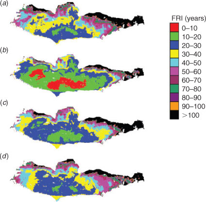
Varying the LFM trend has a noticeable effect on FRI maps (Fig. 9a, b and c). The three trends show similar spatial patterns of high and low values, with dry LFM having the lowest FRI values, followed by wet and constant LFM. This is consistent with Fig. 6c, which showed that large fires are most common for dry, then wet, then constant LFM.

The FRI maps for uniform and spatially correlated ignitions (Fig. 9c and d) demonstrate the importance of using multiple metrics to describe a fire regime. Fig. 6d showed minimal differences in fire size distribution due to the spatial pattern of ignitions, but the FRI maps show clear differences. The northerly western and the eastern portion of SMM show FRIs greater than 100 years in the uniform ignition pattern map (Fig. 9c), and there is a strong contrast with the shorter FRIs seen in the central portion of SMM (FRI between 10 and 20 years). However, roads are concentrated in the northerly western and eastern portions of SMM (Fig. 1c), and although FRI is still highest in these portions of SMM for the correlated ignition pattern map, the area of FRI greater than 100 years is reduced (Fig. 9d). The area of FRI between 10 and 20 years is also reduced, leading to less contrast in values. It is interesting that introducing spatially correlated ignitions serves to decrease the spatial variability evident in the FRI map.

Box plots showing relationships between the natural logarithm of total area burned and the four independent variables are provided in Fig. 10. Increasing the number of ignitions increases the total area burned, with the biggest increase occurring from 1.0 to 4.0 ignitions per year (Fig. 10a). Increasing the number of Santa Ana events also shows increased total area burned, though the relationship is more consistent (Fig. 10b). For LFM trend, dry conditions lead to a much larger total area burned than the wet and constant trends (Fig. 10c). For ignition pattern, uniform ignitions lead to a slightly larger total area burned (Fig. 10d).

Fig. 10.  Box plots for number of ignitions per year (igpy), live fuel moisture (LFM) trend, number of Santa Ana (SA) events per year, and spatial ignition pattern.

Statistical tests demonstrate that the variability seen in the fire size distributions, FRI maps and box plots is very unlikely to arise by chance. All four of the independent variables showed statistically significant relationships with the logarithm of total area burned (P < 0.0001), with number of ignitions explaining the most variance (R² = 0.395, slope = 0.175, intercept = 13.74, Table 3), followed by number of Santa Anas (R² = 0.327, slope = 0.12, intercept = 14.21), LFM trend (R² = 0.08), and spatial ignition pattern (R² = 0.008). The number of ignitions had a steeper slope than the number of Santa Anas and thus is more sensitive to total area burned. All Tukey’s HSD post-hoc pairwise comparisons for LFM were significantly different (P < 0.05), though wet and constant were not also significantly different at the 0.001 level.

Table 3.  Sum of squares and R² for the four independent variables
ig_pattern, categorical variable concerning ignition pattern; LFM, categorical variable concerning live fuel moisture trend used; SA, average annual number of Santa Ana events; igpy, average annual number of ignitions and the significant interactions on ln-transformed total area burned. All are significant at the 0.0001 level

The cumulative variance explained by the four independent variables, without interactions, was 0.8094 (Table 3). All possible interaction terms were added, and then non-significant terms were removed in a stepwise manner using the Akaike information criteria (AIC: Akaike 1974). When the statistically significant interaction effects were included, the explained variance increased to 0.8702 (Table 3). Four interactions were significant at the 0.0001 level: between LFM trend and the number of Santa Anas, LFM trend and the number of ignitions, number of ignitions and the number of Santa Ana events, and the interaction between these three variables. The implications of these interaction terms are discussed below.

Most of the area burned in chaparral shrublands is during Santa Ana events in actuality (Countryman 1974) and also in HFire. Intuitively, increasing the number of ignitions increases the chances that an ignition will occur coincident with a Santa Ana event, up to a point. This may be the mechanism for the importance of the interaction between annual numbers of Santa Ana events and ignitions. One of the text outputs from HFire lists area burned under standard and extreme conditions for each fire. Fig. 11 shows a contour plot representing the percentage of area burned during extreme conditions as a function of number of ignitions and Santa Anas. Several interesting trends are present in the plot. For lower numbers of Santa Anas per year (0.0, 1.0, 2.0), the percentage area burned during a Santa Ana does not change when the number of ignitions increases. Once the number of Santa Ana events per year is 4.0 or greater, increasing the number of ignitions results in increasing percentage area burned during a Santa Ana from 0.450 to 0.6–0.8. For high numbers of both ignitions and Santa Anas, the number of Santa Anas is more sensitive to Santa Ana fraction of total area burned than number of ignitions. This suggests that the system is more limited by the number of wind events rather than the number of ignitions. The FRI maps for the ignitions per year cases also show that once ignitions increase beyond 1.0 per year, FRI remains fairly consistent (Fig. 8).

Fig. 11.  Contour plot of percentage area burned during Santa Ana events, generally showing more sensitivity to the number of Santa Anas as opposed to the number of ignitions.

In the interaction between LFM and the number of Santa Ana events per year, it is clear that the constant trend has the steepest slope and thus is most sensitive to the number of Santa Anas (Fig. 12). The wet LFM trend shows a slightly steeper slope than the dry LFM trend, suggesting that wetter fuels require more wind than drier fuels in order to burn larger amounts of the landscape. The disparity in slope between the constant and wet and dry LFM trends is due to the smaller amounts of total area burned for the lower Santa Ana events per year cases for the constant trend; LFM may have been above a threshold that would lead to large fires under low wind conditions. It is interesting to note that for the zero Santa Ana case, the fire risk in the system appears to be fuel-dominated as the dry LFM trend produces larger fires than the wet and constant trends. But as more Santa Anas are added, the differences in area burned due to LFM trend are reduced (all three LFM trends lead to a mean natural logarithm of total area burned of roughly 16 when the number of Santa Ana events per year increases to 16.0).

Fig. 12.  Box plots for the interaction of LFM (live fuel moisture) and number of Santa Ana (SA) events per year. x axis refers to 0–16 Santa Anas and constant (c), dry (d), and wet (w) LFM. For 0 Santa Anas, the dry LFM trend burned a much larger area than the other trends. At higher numbers of Santa Anas, the weather dominates, and all three LFM trends produce similar total area burned.

The interaction between LFM and the number of ignitions per year shows some similar patterns. All three trends show a large jump in area burned between the one and four ignitions per year cases, and the constant trend shows the steepest slope overall (Fig. 13). However, it is interesting to note that the three different LFM trends have less similar values for the maximum number of ignitions per year than they showed for the maximum number of Santa Anas per year (Fig. 13). The Santa Ana variable was able to dominate the effect of the LFM variable more than the number of ignitions variable did.

Fig. 13.  Box plots for the interaction of LFM (live fuel moisture) and number of ignitions per year (igpy). x axis refers to 0–12 ignitions and constant (c), dry (d), and wet (w) LFM. For 0 ignitions, the constant LFM trend burned a much smaller area than the other trends. At higher numbers of ignitions, the weather dominates, and all three LFM trends produce similar total area burned.

We studied drivers (weather, ignition and fuel) of the long-term fire regime of SMM using the HFire LFSM. Three different aspects of the fire regime were examined: the distribution of fire sizes, the cumulative total fire size, and the spatial patterns of the FRI. These three ways of visualising the output are complimentary, with the maps providing the most detail, and box plots of the total area burned able to efficiently summarise a large number of model runs.

The number of ignitions was most important for predicting total area burned. Haydon et al. (2000) also found high model sensitivity to varying the number of ignitions, especially when values more than ±100% different were tested. In contrast, Oliveras et al. (2005) found minimal sensitivity when the number of ignitions varied between 26 and 110 per year, corresponding to half to two times the current fire ignition frequency per year for their study area. For our data, if we remove the one ignition per year model runs, which are one quarter the current fire ignition frequency of four per year, the R² for this variable drops from 0.395 to 0.138, though this value is still significant. Hence, although increasing the number of ignitions from 4.0 to 12.0 still serves to increase the total area burned, model sensitivity is reduced. A possible explanation is that within a calendar year, prior fires in the fire season may act as fire breaks to later fires, so that more ignitions do not necessarily equate to more area burned. The fire size distribution plot (Fig. 6b) and FRI map (Fig. 8) for the number of ignitions variable support the idea that the biggest difference in fire properties occurs from 1.0 to 4.0 ignitions, with the 4.0, 8.0 and 12.0 ignition cases having more similar output.

This has implications for future fire regimes because ignitions preferentially occur in WUI areas (Radeloff et al. 2005; Syphard et al. 2007), and the WUI will expand in coming decades (Swenson and Franklin 2000). From our model results, it would appear that the increased number of ignitions beyond the current value will have a small effect on burned area. However, increased numbers of people living in the WUI will lead to increased exposure to fire.

The number of Santa Ana events also explained a large amount of variance in total area burned. When the 1.0 ignition per year model runs were removed from the analysis, the R² for number of Santa Anas increased from 0.327 to 0.571 and the overall R² increased from 0.809 to 0.832. Additionally, the Santa Ana variable shows the most consistent increase in area burned in Fig. 6, and the most consistent decrease in FRI in Figs 7–9. This finding heightens the value of initial fire suppression efforts when Santa Ana events are forecast, especially during dry years, if a commensurate increase in total area burned, and loss of life and structures, is to be avoided (Westerling et al. 2004).

The importance of weather-related factors is well established in the fire modelling literature (e.g. Cary et al. 2006). Additionally, a global sensitivity analysis applied to HFire in single-event mode found that wind speed was three times as important as the second-place input (1-h dead fuel moisture) for predicting fire size (Clark et al. 2008).

Climate change is likely to have major effects on ecosystem structure and function, and changing fire regimes will play an important role on many terrestrial landscapes. General circulation models (GCMs) are typically used to predict changes in average temperature and precipitation rather than extreme weather events, but two recent studies have examined changes in Santa Ana event frequencies under different climate change scenarios (Miller and Schlegel 2006; Hughes et al. 2009). Miller and Schlegel (2006) predicted that the peak Santa Ana season will shift from September–October to November–December by the end of the 21st century. Hughes et al. (2009), using a different GCM and methodology, show that Santa Ana frequency has decreased 30% from the 1960s to the 1990s and predict a similar decrease through the mid-21st century. The impact of the number of Santa Ana events on fire regime evident in our research provides impetus for clarifying the response of Santa Ana frequency to climate change.

The sensitivity to LFM trend in HFire is reflected in actual conditions, too. Weise et al. (1998) suggested that fire danger can be approximated using LFM, with low fire danger for LFM > 120%, moderate fire danger for 120% > LFM > 80%, high fire danger for 80% > LFM > 60%, and extreme fire danger for LFM < 60%. The dry LFM trend has values at 60% for August, September and October, whereas LFM does not reach 60% for the wet trend. Dennison et al. (2008) also found an interaction between LFM and Santa Ana events. They found that the seven largest fires in the SMM between 1982 and 2007 occurred when the LFM was below 77%, and Santa Ana winds were present. The net effect of climate change predictions on LFM are unclear, as winter and summer temperatures are predicted to increase by 3° and 1°C respectively, which would tend to dry out fuels, but precipitation is also expected to increase, which may increase LFM (Field et al. 1999). If future fuels are drier, the fire regime will shift to more, larger fires, with a shorter return interval.

The pattern of ignitions demonstrates that viewing different aspects of the fire regime may reveal different trends. The fire size distribution and the total burned area both show minimal differences due to uniform and spatially correlated ignitions. However, the two FRI maps show clear differences. The uniform ignitions map has more areas of high and low FRI, whereas the correlated ignitions map has less contrast.

It is doubtful that native plant species that dominate many shrublands of California will be able to persist under shorter FRIs, because for many fire-dependent chaparral species, there is a threshold in FRI below which plants are not able to successfully regenerate (Zedler et al. 1983). Large areas of FRI below 10 years (highlighted in red in Figs 7–9) occurred in HFire simulations under three conditions: when the number of Santa Ana events was 16.0 per year, when ignitions increased to 12.0 per year, and under dry LFM conditions. The 16.0 Santa Ana per year case is plausible, but unlikely, given current climate change predictions (Miller and Schlegel 2006; Hughes et al. 2009). Future LFM trends are unclear, as discussed above. However, increasing ignitions are almost certain to occur as the WUI expands (Syphard et al. 2007), so there is a risk of type-conversion in the future. Additionally, once a threshold is crossed and native vegetation is type-converted into non-native invasive grasses, further alterations to vegetation patterns and fire regimes are likely through positive feedback cycles (D’Antonio and Vitousek 1992).

Fire regimes are characterised by statistics describing fire size distributions, fire return intervals, and cumulative total area burned. HFire has been shown to model the fire regime of a southern California shrubland (Moritz et al. 2005). In this paper, we evaluated the importance of four physical drivers of these characteristics for southern California. These include the annual number of ignitions, the spatial pattern of ignitions, the annual number of Santa Ana wind events, and LFM trends. Our simulations demonstrated the most significant change in the fire regime metrics arose in response to variations in ignition frequency and extreme fire weather events, whereas fuel moisture trend and ignition pattern had less influence on fire regime metrics. Not surprisingly, the largest cumulative area burned occurred under the most ignitions (12.0 per year), highest wind (16.0 Santa Anas per year), most flammable fuels (dry LFM trend) scenario.

This study demonstrates the promise of HFire as an efficient, mechanistic fire model for long-term fire regime studies. This paper examined steady-state fire regimes for a range of values of the drivers. This provides an initial means to evaluate how fire regimes may change in response to changes in the drivers. More detailed studies of specific scenarios could be obtained by extracting estimates of time-varying drivers from models of climate change or urbanization, which could provide projections for changes in weather parameters, fuel conditions and ignitions, which could then be used as time-varying inputs for HFire.

Incorporation of possible vegetation type conversion (e.g. stochastically driven changes in PNV type based on fire frequency at a site) represents a top priority for the next stage of model development, and will aid in these studies of long-term change. Additionally, more complex variations in fuel model pathways will be explored, involving more chaparral fuel models. Several dynamical upgrades are also of interest. Spotting can increase the overall spread rate of a fire across a landscape, and this has been observed in fire simulation modelling studies (Hargrove et al. 2000). We expect spotting will play an important role in the dynamics of individual fires, including mechanisms for spread of fires into urban areas, but may not have a major impact on long-term statistical metrics. Many potential spot fires are eventually overtaken by the main fire, so that the majority of short-range spotting may not have a major cumulative effect on final fire size (Rothermel 1983), and hence fire size distributions and fire regimes. In addition, upgrades that expand the range of fire regimes that can be investigated are of interest. HFire was developed to model stand-replacing fires in shrubland fuels and thus HFire does not currently model the local, vertical transition of surface fire to crown fire in a forest canopy. As such, the general relationships between physical parameters and fire regimes we observed may or may not hold in ecosystems where this local transition has a large effect on landscape-scale spatial fire patterns and long-term fire regime dynamics.

Modelling is one of few approaches available for investigating fire regime dynamics under future climate change and WUI expansion scenarios. New tools like HFire are useful for exploring sensitivities and possible future scenarios, where the physical parameters governing fire spread are expected to change. Detailed and physically based fire growth algorithms are often considered too complex and computationally intensive for long-term simulations, but HFire’s implementation of the Rothermel (1972) equations allows for multicentury modelling of fire regimes, with simultaneous fires burning on a landscape and regrowth of vegetation between fires.

References

Akaike H (1974) A new look at statistical model identification. IEEE Transactions on Automatic Control 19, 716–723.| A new look at statistical model identification.Crossref | GoogleScholarGoogle Scholar |
Albini FA (1976) Estimating wildfire behavior and effects. USDA Forest Service, Intermountain Forest and Range Experiment Station, General Technical Report GTR-INT-30. (Ogden, UT)
Albini FA, Chase CH (1980) Fire containment equations for pocket calculators. USDA Forest Service, Intermountain Forest and Range Experiment Station, Research Paper RP-INT-268. (Ogden, UT)
Anderson HE (1983) Predicting wind-driven wildland fire size and shape. USDA Forest Service, Intermountain Forest and Range Experiment Station, Research Paper RP-INT-305. (Ogden, UT)
Arca B, Duce P, Laconi M, Pellizzaro G, Salis M, Spano D (2007) Evaluation of FARSITE simulator in Mediterranean maquis. International Journal of Wildland Fire 16, 563–572.