

Identifying high-value tactical livestock decisions on a mixed enterprise farm in a variable environment
Michael Young A B * , John Young C , Ross S. Kingwell A D E and Philip E. Vercoe A B
A
B
C
D
E
Abstract
Australia is renowned for its climate variation, featuring years with drought and years with floods, which result in significant production and profit variability. Accordingly, to maximise profitability, dryland farming systems need to be dynamically managed in response to unfolding weather conditions.
The aim of this study is to identify and quantify optimal tactical livestock management for different weather-years.
This study employed a whole-farm optimisation model to analyse a representative mixed enterprise farm located in the Great Southern region of Western Australia. Using this model, we investigated the economic significance of five key livestock management tactics. These included timing of sheep sales, pasture-area adjustments, rotational grazing, crop grazing and sheep nutrition adjustments.
The results showed that, on the modelled dryland mixed-enterprise farm in the Great Southern region of Western Australia, short-term adjustments to the overall farm strategy in response to unfolding weather conditions increased expected profit by approximately 16%. Each tactic boosted profit by between A$7704 and A$53,171. However, we outline several complexities that farmers must consider when implementing tactics.
The financial gains from short-term tactical management highlighted their importance and farmers’ need to develop and apply those skills. The tactical skills promote business resilience and adaptability in the face of climate uncertainties.
The study highlighted the economic value of dynamic livestock management in response to climate variations, offering farmers in the Great Southern region the means to underpin profitable and sustainable farm practices.
Keywords: AFO, Australian Farm Optimisation Model, discrete stochastic programming, economic optimisation modelling, farming systems, sheep management, tactical farm management, weather variability.
Introduction
Australia is renowned for its climate variation that includes droughts and floods that cause significant production and profit variability (Trompf et al. 2014; Laurie et al. 2019; Feng et al. 2022). This variation can be very challenging for farmers (Heberger 2011), particularly for livestock farmers who must adhere to animal-welfare standards. In mixed-farming systems, livestock and associated pasture production complement cropping activities by utilising crop residues, providing disease and pest breaks, providing weed-management options and improving labour and machinery use efficiency during the year. As such, livestock and pasture production are key components of many farm businesses and farming systems in Australia.
In Western Australia, for example, livestock revenues comprise 21% of average farm total income (Planfarm/BankWest 2019), which is likely to be a greater proportion of the total profit because the livestock enterprise typically incurs lower costs than does cropping (Planfarm/BankWest 2019). Farmers can adjust their flock structure to focus on either wool or meat production or both, providing market diversification (Young et al. 2020). Moreover, livestock income is often received at different times from cropping income, providing operating cash flow throughout the year. Further benefits of sheep and pasture in the farming system include the rotational benefits of nitrogen-fixing pastures and the ability to use salt-affected areas for sheep feed and shelter (O’Connell et al. 2006). In addition, year-round employment is possible because of the continuous care required for sheep, which is especially important in rural areas, where job opportunities may be limited. Machinery usage can also be improved through sowing and manipulating pastures during the year. Crop residues and spilt or split grain at harvest can be grazed by stock and converted from being a waste to a profit.
Climate variation is a constant challenge to managing mixed-enterprise farming systems in Australia, with the incidence of drought especially complicating sheep management when feed and water supplies become increasingly scarce and expensive. To handle climate variation, farmers can alter their ‘big-picture’ strategic management to set up a more versatile and diversified enterprise mix of their farm business (Azam-Ali 2007; Kandulu et al. 2012). However, Kandulu et al. (2012) suggested that, in many locations, a sole focus on diversification does not wholly mitigate the financial effects of climate variation. An alternative management method, applicable by farmers to manage their external variations, is to implement short-term tactical adjustments in response to unfolding conditions (Anderson et al. 2020).
Tactical management is most valuable within systems where farmers have a wide portfolio of tactics for use in response to an external change (Cowan et al. 2013). This is the case in mixed-farming systems where there are many livestock tactics that can be implemented throughout the year in response to unfolding weather conditions, including sale or purchase of stock, adjustment of stock liveweight targets, adjustment of grazing management, adjustment of pasture area and pasture manipulation (Young et al. 2022). In mixed crop and livestock businesses, farmers can adjust enterprise allocation, their interactions and relevant tactics to better suit unfolding climate conditions. The efficacy and value of this suite of adjustment or tactics was commented on by Pannell et al. (2000) who discussed the inclusion of risk attitudes and production and price risk in farm analyses. They concluded that the most important aspect of risk management is a farmer’s short-term tactical response to variation in weather and prices. Furthermore, as outlined by Young et al. (2023a), tactical management generates significant opportunities to boost farm profit and/or avoid losses. Their findings were that optimal tactical management can increase profitability by at least 14%. However, the large array of possible tactics within mixed-enterprise farm systems can significantly complicate management, especially when combined with the constantly changing and evolving nature of farming systems. It is challenging for farmers to identify the optimal suite of tactics to apply in different circumstances during a production year or suite of years.
Despite the likely benefit of research that focuses on identifying appropriate tactical livestock management, previous research on mixed-enterprise farming systems in Western Australia has mostly focused on tactical management for crops. Topics include the tactics regarding the time of sowing, land use and rotation choice and nitrogen application (Kingwell et al. 1993; Abrecht and Robinson 1996; Chen et al. 2009; Doole and Weetman 2009). Furthermore, much of this work was conducted over a decade ago and farming systems and technologies have evolved significantly since then. Research on livestock management has either assumed that every year is the same (Kopke et al. 2008; Bathgate et al. 2009; Young et al. 2010, 2020, 2022) or when year-to-year variation has been included, management has not been optimised and, frequently, the tactical-management options have been over-simplified (McGrath et al. 2016; Godfrey et al. 2019). For example, supplements are always fed to sheep once they reach a threshold-condition score, rather than considering the marginal costs and benefits of the supplementary feed. The paucity of Australian studies that examine, in a mixed-enterprise whole-farm setting, the economic ramifications of tactical management of livestock is a gap in our knowledge.
Given Australia’s variable climate (Feng et al. 2022), the economic importance of livestock in Western Australian farm businesses (Planfarm/BankWest 2019), the profitability of tactical crop management (Kingwell et al. 1993), and the multitude of tactical livestock options (Young et al. 2022), we hypothesise that the optimal implementation of livestock tactics in modern mixed-enterprise farming systems will provide worthwhile increases in farm profit.
Knowing the value of tactics allows farmers to prioritise their management actions. For example, if it is optimal to sell dry ewes in a drought year, but the added profit is small, then a time-pressed farmer can confidently disregard this tactic without major impacts on their business profitability. However, if the tactic results in large changes in profit then, this would indicate that it is highly worthwhile for a farmer to learn and execute this selling tactic.
In this paper, we apply a whole-farm optimisation model that, first, represents year-to-year variation and, second, includes an extensive array of tactical management options tailored to that variation. The model is used to identify and quantify optimal tactical livestock management for different weather-years.
Methods
Model description
The whole-farm model called Australian farm-optimisation model (AFO) is applied in this study. AFO is a whole-farm linear programming model that supersedes the popular MIDAS model (Kingwell and Pannell 1987; Pannell 1996; Kopke et al. 2008; Bathgate et al. 2009; Kingwell 2011; Young et al. 2011, 2020; Thamo et al. 2013). A brief summary of the model is provided below. For a more thorough description, see the model documentation at https://australian-farm-optimising-model.readthedocs.io/en/latest/index.html.
The model represents the economic and biological detail of a farming system, including modules for rotations, crops, pastures, sheep, crop residues, supplementary feeding, machinery, labour and finance. Furthermore, it includes land heterogeneity by considering enterprise rotations on a range of soil classes/land-management units (LMU) (Fig. 1). AFO was selected as an appropriate tool to evaluate optimal tactical livestock management in a mixed-enterprise, broad-acre farming system for several reasons. First, it includes year-to-year climate variation and a large relevant range of tactical management options including adjusting the number of stock, altering rotations, altering stock liveweights, selling livestock, altering supplementary feeding, manipulating grazing timing and intensity, deferring pastures, and crop grazing. Second, AFO leverages powerful algorithms to efficiently identify the optimal management for a given farm system. Finally, AFO also has detailed feed budgeting modules that help identify the optimum utilisation of feed sources across the whole farm.

Year-to-year weather variation
Weather variation can be represented in multiple ways using AFO. Importantly, on the basis of the findings of Young et al. (2023a) and Young et al. (2023b), we adopt the four-stage single-sequence stochastic program with recourse (4-SPR) model, housed within AFO, to examine the role and value of tactical livestock decisions on a mixed-enterprise farm in a variable environment. As discussed by Young et al. (2023b), ‘4-SPR represents the farm system with multiple discrete states where each state represents a different weather-year that can have separate inputs to reflect different prices and weather conditions. All states begin from a common point that is determined by the weighted average of the end of all the weather-years, but then these weather-years separate at multiple nodes during the production year when information becomes known to unveil the particular nature of that weather-year. Once a weather-year has been identified, subsequent decisions can be differentiated based on the known information about that given weather-year’ (p. 6). The eight-stage multi-sequence stochastic program with recourse (8-SPR), also available in AFO, was shown to yield expected results similar to those of the 4-SPR model, but significantly increased execution and interpretation time (Young et al. 2023b). Thus, for this analysis, the 4-SPR model was selected as the optimal tradeoff between time and accuracy. However, it should be noted that the 4-SPR model does not accurately reflect how the outcome of the previous year affects tactical management in the current year. As such, optimal implementation of tactics on farm may differ slightly from that reported in this study, as a response to the outcome of the previous year. Refer to Young et al. (2023b) or to the AFO documentation for more information about the handling of weather variation in AFO.
Objective
AFO has the capacity to represent a farmer’s risk attitude in response to uncertainty or variability. However, in this study we assume a risk neutral attitude. Accordingly, the objective used in this study was to maximise the net cash flow, minus the cost of depreciation, and minus the opportunity cost on the farm assets (excluding land). The opportunity cost is not incurred by the farmer; thus, it is not included in the profit reported in the results. However, the opportunity cost does need to be considered when identifying the optimal farm management to ensure that a minimum return on assets is received. For example, extra stock will not be included in the optimal solution, unless the return achieved is greater than the opportunity cost of their capital value.
Feed budget
In AFO, the supply side of the feed budget comprises green and dry pasture on arable land areas, green and dry pasture on non-arable land areas, pasture on crop paddocks prior to destocking for seeding, early season crop grazing, standing crop fodder, crop residues remaining after harvest and a range of supplementary feeds.
The biology and logistics of pasture production and utilisation represented in AFO are as follows:
Pasture growth rate (PGR) is dependent on pasture leaf area, which is quantified by the level of feed on offer (FOO, kg of DM/ha). Additionally, PGR for each pasture type varies with the life cycle phase of the pasture species, soil moisture, sunlight and level of growth modifier applied. All are quantified by their land-management unit (LMU), time of year and weather-year.
The available FOO depends on grazing intensity.
The mobilisation of below-ground reserves (germination) of annual pastures at the break of season is dependent on the seed bank. The seed bank is controlled by the rotation in which the pasture is grown and varies with the LMU.
The mobilisation of below-ground reserves of perennial pastures at the break of season can also be adjusted by rotation. However, perennials usually are not grown in rotation with crops.
The intake of animals grazing pasture depends on FOO and diet dry-matter digestibility (DMD).
The digestibility of the diet selected by animals grazing green pasture depends on the sward digestibility and the animal’s capacity for selective grazing. Sward digestibility varies depending on the pasture species, the time of year and the LMU. Selectivity depends on FOO and grazing intensity.
Dry pasture that is not consumed is deferred to later in the year, with a reduction in both quality and quantity. Livestock can select a higher-quality diet when first grazing the dry pasture, but quality reduces with extra grazing.
Livestock trample both green and dry pasture while foraging.
The risk of resource degradation increases when ground cover is lower, so there is a minimum limit to ground cover during both the green and dry phases of the year.
The decision variables optimised in AFO and that represent the above biology are the following:
Rotation phases in which pasture can be grown on each LMU.
FOO profile during the year that is represented by a discrete range of FOO levels at the start of each feed period.
Grazing intensity and the variation during the year that is represented by a discrete range of the severity of defoliation in each feed period.
Level of growth modifiers (nitrogen or gibberellic acid) applied to the pasture.
Quantity of dry feed consumed from each of two dry-feed quality groups in each feed period.
Pasture on non-arable areas is modelled as above with a few additions. First, pasture on non-arable area is represented as a continuous annual pasture. Second, pasture on non-arable areas of cropping paddocks is not available for grazing until after harvest and, therefore, it goes into the low-quality dry-feed pool. Accordingly, pasture on non-arable areas of crop paddocks does not receive any farm inputs.
Pasture on crop paddocks before seeding is represented as a pre-specified quality and maximum quantity available each day on the area that is yet to be seeded, with the additional requirement that pasture must be destocked 10 days prior to seeding to allow time for an effective knockdown spray.
Crop grazing is an option that allows stock to graze green crop from June until August. Green crops have a higher energy content than does green pasture and grow more erect, allowing for easier grazing, meaning that a lower crop FOO is required to meet the livestock needs. However, for every kilogram of crop biomass consumed yield is reduced by 150 g per hectare, with a corresponding effect on stubble production.
At the end of the growing season, AFO has the option of harvesting each crop, which leaves stubble for stock consumption, or crops can be left standing for fodder grazing. Stubble and fodder are modelled in the same way, as follows: in general, sheep graze crop residues selectively, preferring the higher-quality components. Thus, they tend to eat grain first, followed by leaf and, finally, stem. To allow the optimisation of the quantity of the stubble grazed, and to reflect selective grazing, the total crop residues are divided into 10 categories. The higher categories are of better quality but generally of lower quantity. Consumption of a higher-quality category allows the consumption of a lower category (e.g. sheep cannot consume any of Category B until some of Category A has been consumed).
The total mass of crop residues at first grazing (harvest for stubble and an inputted date for fodder) is calculated as a product of the biomass, harvest index and proportion harvested. Over time, if the feed is not consumed, it deteriorates in quality and quantity because of adverse effects of weather and the impact of sheep trampling.
Supplementary feeding is the supply of additional feed to livestock, primarily grain and hay (which are both represented in the model). Supplementary feeding is commonly used to help meet production targets, such as lamb growth rates prior to sale, or to fill the feed gap to allow higher stocking rates during the summer and autumn months when pastures and crop residues are limiting. Additionally, feeding supplements can be used as a tactic to allow pastures to be deferred early in the growing season, which increases subsequent pasture growth rates. Grain and hay as supplementary feeds can either be grown on farm or purchased from another farmer at a farm-gate price (i.e. net price of a product after selling costs have been subtracted) plus the transaction and transport costs.
The demand side of the feed budget comprises livestock nutritional needs. AFO generates production parameters for livestock under a range of different conditions. These are represented as different decision variables that allow the optimisation of a wide range of management decisions. Each animal has an energy requirement and intake capacity that depend on liveweight/nutrition targets, genetics, gender, physiological state and age.
A powerful and advanced feature of AFO is its ability to optimise livestock liveweight/nutrition profiles. AFO does this by generating production parameters for animals following a range of nutrition profiles (up to 2000 profiles for each class of sheep can be concurrently evaluated). The range of nutrition level is represented by profiles that are continuous for the entire year. At the end of the nutrition cycle (year), the range of final liveweights are ‘condensed’ back to a range of starting weights for the start of the next nutrition cycle. This capacity allows AFO to feed animals differently on the basis of reproduction, sale goals and feed supply based on land-use selection.
The feed requirement (as measured by metabolisable energy) of each animal is a minimum constraint in the AFO matrix and sufficient feed must be available for each animal that is part of the optimal solution. The feed selected in the optimal solution must also be of sufficient quality that the quantity required to meet the animal’s energy needs is within the intake capacity of that animal, which is represented as a maximum constraint on the volume of feed an animal can consume.
Cross subsidisation of volume is a problem that can occur in the feed budgets of linear programming models. Cross-subsidisation occurs if animals with divergent quality requirements are constrained by single energy and volume constraints; the single constraint is termed a feed pool. For example, consider two animals, one losing 100 g/head.day and one gaining 150 g/head.day. The first animal can achieve its target on low-quality feed, whereas the second animal needs high-quality feed. However, if both of these animals were constrained using a single feed pool, then the total energy requirement and total intake capacity is combined, such that feeding medium-quality feed to both animals meets the constraints. This is likely to be the optimal solution because the cost of feed by quality is a convex function and therefore the cost-minimising solution is to provide an average quality to both classes of stock. However, this is not a technically feasible solution.
To reduce the possibility of cross-subsidisation of volume, while still limiting model size, the energy-requirement and maximum-volume constraints are applied in multiple nutritive value pools, each spanning a small range of nutritive value (where nutritive value = ME requirement/volume capacity). This is more efficient in reducing model size and complexity than having a feed pool for each animal class.
Overview of the farm system
AFO was calibrated to represent a typical farm in the medium-rainfall zone of the Great Southern region of Western Australia. The Great Southern region was selected for two reasons. First, the region has been modelled previously for a variety of analyses (Young 1995; Poole et al. 2002; Young et al. 2011; Trompf et al. 2014) and, thus, the farm data required are more readily available. Second, the Great Southern region contains the largest breeding ewe population (5.6 million head) in Australia (Meat and Livestock Australia 2022); so, the selection of this main sheep-production region helps ensure the study findings are likely to be relevant to many sheep producers.
Through formal discussions (Human ethics Approval number ET000181) with local farm consultants, the model was calibrated to represent current farm-management technology, including machinery complements, herbicides and fertilisers used and rates applied. Tasks contracted and crop and livestock options considered are all consistent with those used by farmers in the modelled region (Tim Trezise, pers. comm., Ed Rigall, pers. comm.).
The Great Southern region in Western Australia is characterised by winter-dominant rainfall (400–650 mm) and a 6-month growing season that supports a mix of cropping and livestock enterprises. Weather variance in the region was approximated by eight discrete states of nature (see Table 1). The model represents a typical 2130 ha farm that includes three LMUs (Table 2). The calibration of crop and pasture inputs was completed through a combination of simulation modelling and consultation with experts. The growth rate of the pastures and yield of crops in each rotation were generated using AusFarm, a simulation model (Moore et al. 2007), with the output for each individual year being simulated and then allocated to a relevant weather-year (Table 1). The simulation-model outputs, grouped by weather-year categories, were reviewed by a local agronomist who applied broad brush scaling to align the yields with farmer practice. Climate data were sourced from the Kojonup weather station (BOM Station 10582) over the period from 1970 to 2020. Soil data representing the land management units defined in Table 2 were sourced from existing data in the APSOIL database (Dalgliesh et al. 2012). Other key features of the modelled farm are shown in Table 3. The standard prices for wool, meat and grain used in the analysis were based on the 70th percentile prices received over the past 13.5 years for wool, 18.5 years for meat and 14 years for grain (Source: Mecardo 2023) Tables 4 and 5.
| Code for weather-year | Definition of each weather-year | Probability of occurrence (%) | Growing season rainfall | Crop yield scalar | |
|---|---|---|---|---|---|
| z1 | Early break with follow up rains and a good spring. | 24 | 447 | 1.2 | |
| z2 | Early break with follow up rains and a poor spring. | 20 | 346 | 1.0 | |
| z3 | Early break that turns out to be a false break, but is followed by a good spring. | 8 | 416 | 1.22 | |
| z4 | Early break that turns out to be a false break and is followed by a poor spring. | 4 | 294 | 0.87 | |
| z5 | Medium break with follow-up rains and a good spring. | 14 | 448 | 1.05 | |
| z6 | Medium break with follow-up rains and a poor spring. | 16 | 392 | 0.83 | |
| z7 | Late break with follow-up rains and a good spring. | 4 | 477 | 0.95 | |
| z8 | Late break with follow-up rains and a poor spring. | 10 | 337 | 0.65 |
Yield scalar is the relationship between yield in the given weather-year and the average yield. This was calculated using the output of APSIM modelling using Kojonup climate and soil data from 1970 to 2019.
Early break (i.e. start of the growing season): before 5 May; medium break: between 5 May and 25 May; late break: after 25 May.
Good spring, above the median (86 mm) rainfall for September and October; poor spring, below the median rainfall.
False break, pasture feed on offer reaches 500 kg/ha, followed by 3 weeks of no growth.
| Soil class | Description | Arable (%) | Grazing area (ha) | |
|---|---|---|---|---|
| Deep sands | Deep sands, but not waterlogged. Over mottled clay. | 100 | 150 | |
| Sandy gravels | Gravels and sandy gravels down to 50 cm over clay or gravelly clay. | 80 | 1230 | |
| Sandy loams | Sandy loam, loamy sand over clay rock outcropping in landscape. | 80 | 750 |
| Farm size (ha) | 2130 | |
| Time of lambing | ‘Spring’ lambing (lambing starts mid-July) | |
| Pregnancy scanning management | Scanning for pregnancy status only | |
| Sheep liveweight | Nutrition profile is optimised by AFO | |
| Sheep genetics | Medium-frame Merino | |
| Standard reference weight (kg) | 55 | |
| Fibre diameter (μ) | 20 | |
| Canola yield (t/ha) A | ||
| Roundup-ready | 2.6 | |
| Standard (non-GM) | 2.2 | |
| Wheat yield (t/ha) A | 4.5 | |
| Barley yield (t/ha) A | 5.0 | |
| Oat yield (t/ha) A | 4.5 | |
| Hay yield (t/ha) A | 8.0 | |
| Lupin yield (t/ha) A | 2.5 | |
| Faba bean yield (t/ha) A | 3.0 |
| Prime lamb A (A$/kg) | Store lamb B (A$/kg) | Export wether C (A$/hd) | Breeding ewe D (A$/hd) | Mutton (A$/kg) | Wool E (c/kg) | |
|---|---|---|---|---|---|---|
| 6.98 | 6.24 | 112 | 127 | 4.87 | 1432 |
Source: Mecardo (2023).
| Canola (A$/t) | Wheat (A$/t) | Barley (A$/t) | Oats (A$/t) | Lupins (A$/t) | Faba bean (A$/t) | |
|---|---|---|---|---|---|---|
| 566 | 301 | 283 | 235 | 305 | 350 |
Source: Mecardo (2023).
Tactics comparison
Farmers have a large array of tactics they can apply as the year unfolds and many of these are represented in AFO. However, to economise on word count, in this study, we only examined some of the more common livestock tactics and so focus on the following tactics:
Sale quantity and timing – additional classes of sheep can be sold or retained in response to the unfolding years condition.
Pasture area and rotation – the area of pasture can be adjusted on the basis of the time of break and pasture can be established in paddocks with different land-use histories that affect germination (e.g. continuous pasture has a higher germination than pasture following multiple years of crop).
Grazing management – depending on the unfolding year stock can follow different grazing management (e.g. pasture can be deferred for longer in weather-years in which pasture growth is limiting).
Crop grazing – crops can be grazed early in the growing season when pasture is limiting, or to allow pasture to be deferred.
Stock nutrition profile – animals can gain more weight in a good year and lose more weight in a poor year.
To understand the value of each tactic, we compared the profitability of the farm with the tactic versus a farm with a ‘minimal’ level of the tactic. A minimal level of each tactic was used as the comparison because it is impossible for a farmer not to change some part of their management in response to changing conditions among years. For example, in a poor year, even a farmer with a largely ‘set and forget’ style of management will be forced to accommodate some management mix of feeding more supplements, allowing animals to lose weight or selling some animals as a response to the lower pasture production. The ‘minimal’ scenario is defined below.
Sale quantity and timing – in the ‘minimal’ scenario, sale quantity and timing are forced to be the same in each weather-year.
Pasture area and rotation – in the ‘minimal’ scenario, rotation selection is forced to be the same in each weather-year.
Grazing management – in the ‘minimal’ scenario, sheep are forced to graze at a similar intensity on all the paddocks of each LMU. This represents a simple set-stocking management practice. Both sheep liveweight and the quantity of supplement fed can vary among years. The grazing intensity level selected is calculated as the weighted average of the grazing intensities selected in the full model for a given level of FOO, at a given time of the year, on a given LMU, in a given weather-year. It should be noted that in the ‘minimal’ grazing-management scenario, pastures can still be deferred because it was too challenging, in a realistic way, to prevent AFO optimising all short-term grazing-management decisions. This may result in an underestimate of the importance of grazing-management tactics.
Crop grazing – in the ‘minimal’ scenario, crop grazing is not included. Crop grazing was excluded from the ‘minimal’ scenario because this reflects typical management in the target region and, because of difficulties, as discussed below, of representing non-optimal management in an optimising model if crop grazing was included at the weighted average quantity. This assumption about the ‘minimal’ scenario will increase the total value of tactical management relative to using the weighted average-crop grazing quantity; however, the results are relevant to the majority of the farming population in the target region.
Stock nutrition profile – for farmers both actively and not actively implementing tactical management, the nutrition profiles of livestock are likely to change among weather-years. Therefore, to remove any arbitrary impact of setting the livestock nutrition profile in the ‘minimal’ scenario, stock nutrition is optimised by AFO.
AFO is an optimisation model, therefore, even with the constraints applied to the ‘minimal’ scenario, the model will optimise the management within the restricted remaining options that are available. Therefore, the results provided are representative of a skilled operator implementing a less than optimal system. As such, the value of adopting tactical management is likely to be underestimated in our analysis. For example, the livestock nutrition profile is being optimised in the ‘minimal’ scenario and will maximise any opportunities to alter the temporal allocation of feed among classes of stock, while meeting the constraint that the pasture must be grazed at the same intensity in each paddock. Accordingly, the estimates of the role and value of key sheep management tactics should be seen as conservative estimates.
Results
Value of tactics and strategic impact
Dynamically managing farming systems in response to unfolding weather conditions increases expected profit by A$128,000 (16%) (Table 6). Tactical management has a large impact in early break years that have no follow-up rain (z2 and z3) (Table 6). This is largely because in the Great Southern region of Western Australia, false breaks do not affect crop production (Table 1). However, pasture production during the false-break period is significantly reduced. Thus, tactical adjustments have the potential to significantly boost profit in those years.
| Weather-year | Full tactics (×1000) | Minimal tactics (×1000) | Change (×1000) (% in parentheses) | |
|---|---|---|---|---|
| Expected | $904 A | $776 A | $128 (16%) A | |
| z0 | $1345 | $1164 | $181 (16%) | |
| z1 | $990 | $872 | $118 (14%) | |
| z2 | $1068 | $767 | $301 (39%) | |
| z3 | $370 | $106 | $264 (250%) | |
| z4 | $931 | $876 | $56 (6%) | |
| z5 | $624 | $527 | $98 (19%) | |
| z6 | $836 | $778 | $59 (8%) | |
| z7 | $187 | $183 | $4 (2%) | |
| Minimum A | $186 B | $105 B | $81 (44%) B | |
| Maximum | $1344 B | $1164 B | $180 (13%) B |
A farm managed with a full complement of tactics has a different overall strategy from a farm managed with minimal tactics. For example, with tactics, the optimal overall stocking rate is increased by 30% (Table 7). Thus, the change in profit reported in Table 6 is not necessarily a reflection of the importance of including tactics in a given weather-year. For example, other results (not included here) show that the value of tactics in z7 is A$90,000 (105%). Utilising tactics in z7 (a poor weather-year) allows the profit to remain similar, while the strategic stocking rate is increased.
| Full tactics | Minimal tactics | ||
|---|---|---|---|
| Profit (×1000) | A$903.5 | A$775.7 | |
| Stocking rate (dry-sheep equivalents/winter grazed area, DSE/ha) | 18.6 | 14.3 | |
| Supplement fed (t) | 937.3 | 829.8 | |
| Pasture area (%) | 35.6 | 39.2 | |
| Cereal area (%) | 39.4 | 38.7 | |
| Canola area (%) | 25.0 | 22.1 |
All tactics have a significant impact on farm profit (Table 8). However, because of the interactions among the different tactics, the exact value depends on the complement of tactics being applied.
| Item | Crop grazing (×1000) | Pasture grazing (×1000) | Rotation ($’000) | Stock sale (×1000) | |
|---|---|---|---|---|---|
| All in – remove each tactic | A$53 | A$17 | A$28 | A$14 | |
| All out – add each tactic | A$27 | A$44 | A$30 | A$8 |
All in, calculated by a model with all tactics included, then each tactic removed individually.
All out, calculated by a model with all tactics excluded, then each tactic added individually.
Key tactical decisions
In early break years, it is optimal to increase the canola area by up to 55% and in late-break years, it is optimal to decrease canola area by 55% (Table 9). All of the tactical-rotation adjustments occur on the productive soils (LMU 3 and LMU 4). Sandy soils (LMU 2) are never tactically adjusted and always remain in continuous pasture (Table 9). The difference in rotation selection on the basis of the presence or absence of follow-up rains in early breaks shows that in years with an early break, it is optimal to delay the rotation decision on a proportion of the area until follow-up rains are received. The results in this paper report only the changes in land-use area on each soil type. However, the adjustments are fine-tuned on the basis of the rotation history. This is accounted for in AFO, but, for simplicity, we have not reported the full rotation changes.
| Weather-year | Pasture (ha) | Cereal (ha) | Canola (ha) | |||||||
|---|---|---|---|---|---|---|---|---|---|---|
| LMU2 | LMU3 | LMU4 | LMU2 | LMU3 | LMU4 | LMU2 | LMU3 | LMU4 | ||
| Expected A | 150 A | 108 A | 500 A | 0 A | 720 A | 119 A | 0 A | 402 A | 130 A | |
| z0 | 150 | 95 | 424 | 0 | 537 | 100 | 0 | 598 | 227 | |
| z1 | 150 | 95 | 424 | 0 | 537 | 100 | 0 | 598 | 227 | |
| z2 | 150 | 107 | 475 | 0 | 612 | 209 | 0 | 511 | 67 | |
| z3 | 150 | 107 | 475 | 0 | 612 | 209 | 0 | 511 | 67 | |
| z4 | 150 | 132 | 620 | 0 | 920 | 84 | 0 | 178 | 46 | |
| z5 | 150 | 132 | 620 | 0 | 920 | 84 | 0 | 178 | 46 | |
| z6 | 150 | 99 | 506 | 0 | 956 | 182 | 0 | 175 | 62 | |
| z7 | 150 | 99 | 506 | 0 | 956 | 182 | 0 | 175 | 62 | |
| Minimal tactics B | 64 | 498 | 271 | 86 | 424 | 315 | 0 | 308 | 164 | |
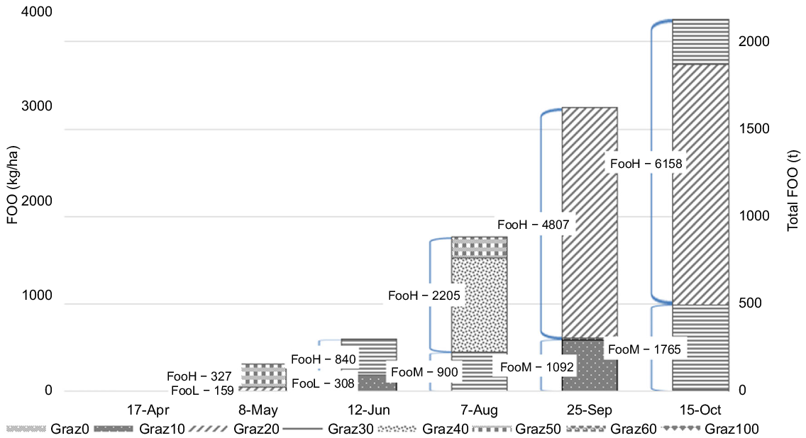
Under minimal tactics, all pasture is grazed at a similar intensity and all paddocks have a similar level of FOO. Optimal management employs rotational grazing, grazing low-FOO paddock lightly to maximise growth (Fig. 2). In early break weather-years, it is optimal to graze pastures heavily early and then defer them by grazing crops.
Full-tactics green-pasture grazing summary for LMU4 and z4. The columns indicate both the total FOO and FOO per hectare at the specified date. The data labels indicate the FOO per hectare of each FOO level. The shaded segments indicate the grazing intensity where Graz100 means grazing all the available feed (including the growth).
The optimal level of crop grazing correlates with the break of season timing, where early break seasons have the highest level of crop grazing (Table 10). After an establishment period, crops can be grazed. However, it is optimal to further delay grazing to increase relative availability of the feed. At low FOO levels, the relative availability of pasture is low, which reduces intake and nutritive feed values for sheep. At low nutritive value, the yield penalty outweighs the value of grazing. Hence, in late-break and false-break years, some of the crop available for consumption is not grazed (Table 10). Crop grazing is economical even in favourable weather-years because the stocking rate is increased, which outweighs the negative impact of yield loss.
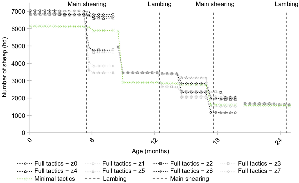
The majority of sales that differ on the basis of weather-year conditions are related to stock less than 18 months of age. Additionally, there are some smaller tactical sales of sheep that include the oldest age group of ewes. Adjusting only the youngest and oldest age group of animals allows the breeding strategy to remain constant, suggesting that destocking of ewes in a poor year is not profitable because of the opportunity cost caused by being understocked in the subsequent years. The farm strategy (minimal tactics) is to sell the heavy proportion of wethers at 8 months of age and the remainders after the second shearing at 18 months of age (Fig. 3). With tactical management included the general strategy is similar however, in years with a false break or a poor spring; a large proportion of the wethers are sold after shearing at 5.5 months of age. Additionally, in years with a false break, a greater proportion of wethers are sold at 8 months of age.
Sheep numbers by age group in each weather-year. Note: There is a gap in the graph at 8 months and 20 months, which is the beginning of the next year, at which point all weather years have the same opening numbers and they can then diverge again.
Implementation of the short-term tactical management increases the optimal winter stocking rate (Table 11), while reducing supplement fed per DSE in five of eight weather-years (Table 12).
Discussion
Australia’s variable climate results in the need to manage its dryland farming systems dynamically to maximise profitability. This paper goes beyond past work, utilising a more comprehensive, current up-to-date farm-optimisation model with a full array of tactical options, to identify the optimal complement of tactical adjustments to apply and their associated profitability. The findings indicated that managing farming systems dynamically in response to unfolding weather conditions is highly profitable, increasing the expected profit by 16% (Table 6). This concurs with the few previous studies that have examined the mixed-enterprise farming system of Western Australia. For example, Young et al. (2023b) showed that including tactical decision-making increases expected farm profit by at least 14%. Kingwell et al. (1993) also showed that implementation of rotation tactics in the wheatbelt region increased expected profit by 22% and Trompf et al. (2014) showed that stocking-rate adjustments due to stock-sale adjustments increased profit by up to A$112,000 depending on the strategic stocking rate. These results illustrated that deterministic models and even stochastic models that do not include tactical adjustments miss a key feature of the management of the farming system and may incorrectly identify optimal activities. Furthermore, from a farmer’s point of view, the key message from all these studies is that a ‘set and forget’ management approach is far from optimal. However, the value of implementing the optimal tactical management outlined in this paper will vary among producers, depending on their current management.
The implementation of tactics can potentially be complex. Farmers must consider that as they implement tactics into their system, their underlying strategy must also be adjusted (Table 7). For example, stocking rate is significantly increased as tactical management is implemented. Additionally, each category of tactics defined in this paper is made up of many suboptions. For example, rotation tactics are defined by LMU and rotation history. The added complexity means that the farm manager must be suitably skilled to identify the type of unfolding season and implement the correct tactics in a timely manner (in the future, monitoring tools such as Pastures from Space may have an important role in assisting farmer to identify the weather-year being experienced). In this analysis, there was no economic cost incurred for the additional skill required to implement tactics because this is farm specific. However, it is a factor that may warrant consideration when interpreting the results. Additionally, because of a large on-farm storage and modest opportunity cost of carrying inputs between years, no cost has been attributed to the potential need to store additional inputs (seed, fertiliser, chemical and supplementary feed) on farm to facilitate tactical land-use adjustments as the weather-year unfolds. Given these factors and each farmer’s unique circumstances, they may want to implement only a subset of the available tactical options. The economic value of implementing an additional tactic varies depending on the complement of tactics being applied (Table 8). However, there is scope to further examine the interactions among tactics; in the eight scenarios tested in this paper, an additional tactic was worth between A$7704 and A$53,171. This indicates that a farmer can improve farm profitability and robustness in a variable climate by implementing only a subset of the available tactics.
This study was based on a ‘typical’ farm in the Great Southern region of Western Australia. Like the study region, many farming regions within Australia have significant weather variation. Therefore, we expect that the conclusion that implementing tactical management can increase profit will be applicable to a wide range of farm systems beyond the target of this analysis, provided those regions have variation in weather among years. The value of different tactics is highly likely to vary across regions and also among farms, so the results need to be implemented with care for a given farm. However, the modelling method could be used to generate customised results for a specific farm.
There are several technologies that may warrant further investigation as tools to aid the management process. First, improved seasonal forecasting is likely to be valuable because it can provide decision makers with an early indication of the weather-year being experienced, allowing improved tactical management. Second, low-cost instrumentation or data sources that provide accurate indicators of in situ impacts of an unfolding season (e.g. pasture growth rates, FOO, animal weight change) will facilitate tactical decision-making, and are likely to increase the returns (or avoid losses) from such decision-making.
Our results are based on expected long-term prices and market conditions. However, short-term price fluctuations, if they can be predicted, may mean that farmers could implement extra tactical adjustments to those reported in this paper to increase returns. This would be a valuable direction for future research.
Conclusions
Short-term adjustments to the overall farm strategy in response to unfolding weather conditions can result in substantial improvements in expected profit on dryland mixed-enterprise farms in the Great Southern region of Western Australia (by approximately 16%). Benefits stem, first, from capitalising on knowledge about the profitability of different decision tactics tailored to the unfolding weather conditions. Second, the benefits accrue from more optimally selecting the underlying farm management strategy of the farm business. Deterministic models and even stochastic models that do not include activities for tactical adjustments miss this key feature of the system and may incorrectly identify optimal activities.
Data availability
All data used in this paper have been referenced and is publicly available. The model/code used for this paper can be licensed to others on request.
Declaration of funding
The authors thank the Department of Primary Industries and Regional Development, WA for financial support through the Sheep Industry Business Innovation project.
Acknowledgements
The authors thank Katelyn Bruinsma for final edits. This paper forms part of the PhD thesis of Michael Young (2023).
References
Abrecht DG, Robinson SD (1996) TACT: a tactical decision aid using a CERES based wheat simulation model. Ecological Modelling 86, 241-244.
| Crossref | Google Scholar |
Anderson WK, Brennan RF, Jayasena KW, Micic S, Moore JH, Nordblom T (2020) Tactical crop management for improved productivity in winter-dominant rainfall regions: a review. Crop and Pasture Science 71, 621-644.
| Crossref | Google Scholar |
Azam-Ali S (2007) Agricultural diversification: the potential for underutilised crops in Africa’s changing climates. Rivista di Biologia/Biology Forum 100, 27-28.
| Google Scholar |
Bathgate A, Revell C, Kingwell R (2009) Identifying the value of pasture improvement using wholefarm modelling. Agricultural Systems 102, 48-57.
| Crossref | Google Scholar |
Chen W, Bell RW, Brennan RF, Bowden JW, Dobermann A, Rengel Z, Porter W (2009) Key crop nutrient management issues in the Western Australia grains industry: a review. Soil Research 47, 1-18.
| Crossref | Google Scholar |
Cowan L, Kaine G, Wright V (2013) The role of strategic and tactical flexibility in managing input variability on farms. Systems Research and Behavioral Science 30, 470-494.
| Crossref | Google Scholar |
Doole GJ, Weetman E (2009) Tactical management of pasture fallows in Western Australian cropping systems. Agricultural Systems 102, 24-32.
| Crossref | Google Scholar |
Feng P, Wang B, Macadam I, Taschetto AS, Abram NJ, Luo J-J, King AD, Chen Y, Li Y, Liu DL, Yu Q, Hu K (2022) Increasing dominance of Indian Ocean variability impacts Australian wheat yields. Nature Food 3, 862-870.
| Crossref | Google Scholar |
Kandulu JM, Bryan BA, King D, Connor JD (2012) Mitigating economic risk from climate variability in rain-fed agriculture through enterprise mix diversification. Ecological Economics 79, 105-112.
| Crossref | Google Scholar |
Kingwell R (2011) Managing complexity in modern farming. Australian Journal of Agricultural and Resource Economics 55, 12-34.
| Crossref | Google Scholar |
Kingwell RS, Pannell DJ, Robinson SD (1993) Tactical responses to seasonal conditions in whole-farm planning in Western Australia. Agricultural Economics 8, 211-226.
| Crossref | Google Scholar |
Kopke E, Young J, Kingwell R (2008) The relative profitability and environmental impacts of different sheep systems in a Mediterranean environment. Agricultural Systems 96, 85-94.
| Crossref | Google Scholar |
Meat and Livestock Australia (2022) 7.6 million lambs to hit the market this spring. Available at https://www.mla.com.au/news-and-events/industry-news/7.6-million-lambs-to-hit-the-market-this-spring/#:~:text=The%20largest%20breeding%20ewe%20population,NSW%20at%204.8%20million%20head [accessed January 2023]
Mecardo (2023) Percentiles – April 2023. Available at https://mecardo.com.au/percentiles-april-2023/ [accessed January 2023]
Moore AD, Holzworth DP, Herrmann NI, Huth NI, Robertson MJ (2007) The Common Modelling Protocol: a hierarchical framework for simulation of agricultural and environmental systems. Agricultural Systems 95, 37-48.
| Crossref | Google Scholar |
O’Connell M, Young J, Kingwell R (2006) The economic value of saltland pastures in a mixed farming system in Western Australia. Agricultural Systems 89, 371-389.
| Crossref | Google Scholar |
Pannell DJ (1996) Lessons from a decade of whole-farm modeling in Western Australia. Applied Economic Perspectives and Policy 18, 373-383.
| Crossref | Google Scholar |
Pannell DJ, Malcolm B, Kingwell RS (2000) Are we risking too much? Perspectives on risk in farm modelling. Agricultural Economics 23, 69-78.
| Google Scholar |
Planfarm/BankWest (2019) Planfarm Bankwest Benchmarks: 2018-2019. Available at https://static1.squarespace.com/static/5cd3c30baf468328f012b132/t/5d522fec77ab8300016a097b/1565667337641/Planfarm+Benchmarks+2018-2019.pdf [accessed January 2023]
Poole ML, Turner NC, Young JM (2002) Sustainable cropping systems for high rainfall areas of southwestern Australia. Agricultural Water Management 53, 201-211.
| Crossref | Google Scholar |
Thamo T, Kingwell RS, Pannell DJ (2013) Measurement of greenhouse gas emissions from agriculture: economic implications for policy and agricultural producers. Australian Journal of Agricultural and Resource Economics 57, 234-252.
| Crossref | Google Scholar |
Young JM, Thompson AN, Kennedy AJ (2010) Bioeconomic modelling to identify the relative importance of a range of critical control points for prime lamb production systems in south-west Victoria. Animal Production Science 50, 748-756.
| Crossref | Google Scholar |
Young JM, Thompson AN, Curnow M, Oldham CM (2011) Whole-farm profit and the optimum maternal liveweight profile of Merino ewe flocks lambing in winter and spring are influenced by the effects of ewe nutrition on the progeny’s survival and lifetime wool production. Animal Production Science 51, 821-833.
| Crossref | Google Scholar |
Young M, Kingwell R, Young J, Vercoe P (2020) An economic analysis of sheep flock structures for mixed enterprise Australian farm businesses. Australian Journal of Agricultural and Resource Economics 64, 677-699.
| Crossref | Google Scholar |
Young M, Vercoe PE, Kingwell RS (2022) Optimal sheep stocking rates for broad-acre farm businesses in Western Australia: a review. Animal Production Science 62, 803-817.
| Crossref | Google Scholar |
Young M, Young J, Kingwell R, Vercoe P (2023a) Improved whole-farm planning for mixed-enterprise systems in Australia using a four-stage stochastic model with recourse. Australian Farm Business Management 20, 1.
| Google Scholar |
Young M, Young J, Kingwell RS, Vercoe PE (2023b) Representing weather-year variation in whole-farm optimisation models: four-stage single-sequence vs eight-stage multi-sequence. Australian Journal of Agricultural and Resource Economics 68, 44-59.
| Crossref | Google Scholar |