

Automated Editing of Radio Interferometer Data with pieflag
Enno MiddelbergAustralia Telescope National Facility, Epping NSW 1710, Australia. Email: enno.middelberg@csiro.au
Publications of the Astronomical Society of Australia 23(2) 64-68 https://doi.org/10.1071/AS06004
Submitted: 10 January 2006 Accepted: 15 March 2006 Published: 17 May 2006
Abstract
Editing radio interferometer data, a process commonly known as ‘flagging’, can be laborious and time-consuming. One quickly tends to flag more data than actually required, sacrificing sensitivity and image fidelity in the process. I describe a program, pieflag, which can analyze radio interferometer data to filter out measurements which are likely to be affected by interference. pieflag uses two algorithms to allow for data sets which are either dominated by receiver noise or by source structure. Together, the algorithms detect essentially all affected data whilst the amount of data which is not affected by interference but falsely marked as such is kept to a minimum. The sections marked by pieflag are very similar to what would be deemed affected by the observer in a visual inspection of the data. pieflag displays its results concisely and allows the user to add and remove flags interactively. It is written in python, is easy to install and use, and has a variety of options to adjust its algorithms to a particular observing situation. I describe how pieflag works and illustrate its effect using data from typical observations.
Keywords: methods: data analysis
Introduction
Data editing, to rid data sets from measurements which are obviously wrong (for whatever reason) or affected by external factors, is a widely accepted practice in all branches of science. Radio astronomical measurements, in particular at frequencies below 5 GHz, can be severely affected by emission from man-made transmitters, which is then known as radio frequency interference (RFI). Only a few attempts have been made as yet to automate the editing of radio astronomical observations, an example includes the ‘WSRT flagger’ used at the Westerbork telescope 1 . However, it is recognized that powerful RFI mitigation techniques need to be developed for future instruments such as the Square Kilometre Array (SKA; Ellingson 2004).
In radio interferometry, data editing is commonly known as ‘flagging’. RFI-affected data are not discarded but an entry (a ‘flag’) is made in an associated computer file, to indicate that the data are not to be used in further processing. When large amounts of data have to be handled, data flagging can be very laborious and dull. This can lead to situations in which one either flags too many or too few data, sacrificing good data in the former case or accepting a degradation of the quality of the observations in the latter.
The automation of flagging requires the creation of a measure which indicates what is ‘good’ data, and then the observed data need to be compared to this measure. Both of these requirements have to work in a variety of circumstances, and assumptions which may work well in one case can be invalid in another.
In pieflag 2 , two algorithms are implemented to detect RFI-affected data made under a variety of circumstances. Two steps of postprocessing extrapolate the flags which were created by pieflag to points close in time. This yields a safety margin around RFI-affected data and picks up those data which are likely to be affected as well but have not been found by the finding algorithms.
pieflag has been designed to read data processed with miriad (Sault et al. 1995), which is the standard data reduction package for observations made with the Australia Telescope Compact Array (ATCA). However, it will work on (u, v) data from other interferometers as well, when these are converted into the miriad format. I note that the algorithms presented here are not specific to interferometric observations. Time series of single-dish radio telescope data could be analyzed in the same fashion.
I will first describe the details of the algorithms used to detect RFI and to generate flags, then the display of the results and how the flags are applied to data sets, followed by an assessment of the limitations, a description of usage, and some examples.
How pieflag Works
pieflag reads in data from miriad data sets and tries to identify RFI-affected sections of data by comparing the visibility amplitudes of each frequency channel to a channel in the spectrum which is known to contain little or no bad data (the reference channel). Consequently, the data must be bandpass-calibrated before pieflag is used. The hypothesis used here is that data are affected mostly by man-made RFI, which typically is limited to very narrow frequency bands (see for example the spectra measured at the ATCA 3 ). This type of RFI thus can be detected when data from different channels are compared. The amplitudes of atmospheric noise and the astronomical signal usually vary between baselines and coordinates at which the telescopes are directed (a ‘pointing’), hence the comparison must be done separately for each baseline and pointing.
The minimum number of parameters pieflag needs to work is the name of a directory with a miriad data set and the number of the reference channel. pieflag works in four steps to generate flags, the first two of which are used to determine which data are deemed to be RFI-affected, and the last two of which transfer the flags to adjacent data which are likely to be affected as well. These four steps are described in the following sections.
Step 1: Amplitude-Based Flagging
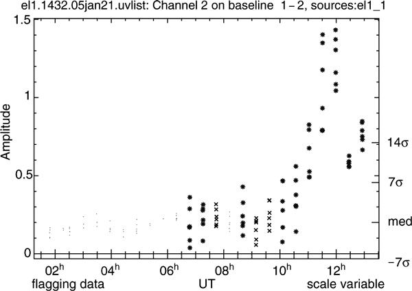
In the first step, pieflag computes the median visibility amplitude of the reference channel, x b,p, for each baseline ‘b’ and pointing ‘p’, and the median of the difference to this median, y b,p. The use of the median and the median of the difference to the median as a measure for the scatter protects the algorithm from outliers in the reference channel. Both the mean and standard deviation can easily be contaminated by single data points with very high amplitudes, and are therefore not suitable. pieflag then calculates the difference of each data point in each channel to x b,p. If the difference exceeds ny b,p, where n is typically around 7, a point is considered suspect and is assigned a ‘badness’ value of 1. If the difference exceeds 2ny b,p, it is deemed certainly bad and is assigned a ‘badness’ value of 2. Amplitude-based flagging is most efficient when the data are dominated by receiver noise or in the presence of very weak astronomical signals. In the presence of strong signals from structured sources, y b,p tends to be too high for the algorithm to detect bad data which deviate only little from the source signal (Figure 4). The badness values are not converted to flags before postprocessing (see Step 3 below).
If the visibility amplitudes in the reference channel have a normal distribution, then 68.2% of the data fall within the range of ± 1σ of the mean. The median of the difference to the median, however, chooses those 50% of the data that fall within the range of x b,p ± y b,p, with y = 0.674σ (this was computed numerically). Hence, in the case of normally distributed amplitudes and n = 7, ny b,p is equivalent to n × 0.674σ = 4.72σ.
Step 2: RMS-Based Flagging
In this step, pieflag calculates the median of the standard deviation, or RMS, in short (typically 2–3 min) sections of reference channel data for each baseline and pointing. The median RMS value, z b,p, is used as a measure of a typical RMS to which the other channels are compared. If the RMS in a section exceeds mz b,p, with typically m = 3, then the entire section is flagged. The concept of badness is not used by this algorithm because groups of points are considered and not single points. This algorithm can find bad data even in the presence of a strong source signal, and therefore complements the amplitude-based flagging. However, terrestrial and solar interference can increase amplitude levels without much effect on the RMS on short timescales, which then is unnoticed by this algorithm (but likely to be detected by the first).
Step 3: Postprocessing to Find Small Clusters of Bad Points
If both amplitude- and RMS-based flagging have been applied, pieflag’s internal tables contain information about the badness of some points as derived by amplitude-based flagging, and information about which parts of the data should be flagged as derived from RMS-based flagging. To turn the badness values into flags, the running sum of the badness values in a 1 min window is calculated in each channel and on each baseline. If the sum exceeds 1, the window is flagged. This procedure will tolerate single, moderate outliers (one value with badness 1 within one minute), but will flag the entire window if two moderate outliers, or one point with badness 2, occur within a minute. It also flags a small margin around the bad data. This algorithm is applied irrespective of pointings, because it is assumed that data are affected irrespective of changes of pointings, at least on such short timescales.
Step 4: Postprocessing to Find Larger Clusters of Bad Points
When developing the flagging algorithms, it was found that often a few affected data points were not found during times with strong interference. For example, some data points in Figure 2 at 11:50 h have amplitude and RMS levels which are not suspicious, given that most of the data in that channel have similar amplitudes. However, considering the high levels of interference immediately surrounding these data, one would certainly flag them as well, if the editing was done manually.
One can argue that if any data has not been detected by the procedures described above, they should not be flagged. Also, considering that should these data be affected at all they would have only minuscule effects on the final result, it seems pointless to flag them. On the other hand, it is known in experimental sciences that bad data can be worse than no data, and that discarding possibly good data as a safety measure is acceptable (to some degree). I also point out that the amount of data additionally flagged in this and the previous step is of the order of a few percent at most, hence the sensitivity loss is negligible. It therefore is a matter of personal taste and level of caution whether or not to apply this step.
The flags are gridded into bins with a width of 30 s and convolved with a boxcar function with a width of typically 20 min. The amplitude of the convolution is a function of the fraction of data which have been flagged in any period of 20 min, and the maximum possible value is predictable. If the fraction exceeds a threshold (typically 0.15 of the maximum), the entire window is flagged. An additional benefit of this procedure is that a larger safety margin is flagged around extended periods of bad data. This step also is carried out irrespective of pointings.
Except for step 3, each of the steps above is adjustable to one’s needs. Adjustable parameters are the multiplication factors n and m in the search for bad data, the width of the sections in which the RMS is calculated in RMS-based flagging in step 2, and the width of the boxcar function and the threshold above which the entire window is flagged in step 4. Furthermore, steps 1, 2, and 4 can be skipped.
Display of the Results
pieflag displays its results to the user for iterative adjustment of the parameters (Figure 1). The visibility amplitudes of one baseline and one channel are displayed, either from all pointings at once, or from one pointing only. The latter is more instructive when attempting to understand why data have been flagged. In the single source mode, x b,p, x b,p ± ny, and x b,p ± 2ny are indicated on the right of the plot. Although the plotting stage allows interactive flagging and unflagging using mouse and keyboard controls, its primary intent is to allow one to inspect the results. Consequently, once pieflag is tuned to fit one’s data, it can be run without plotting.
|
|
Application of Flags to the Data
pieflag does not modify the flagging tables of miriad data sets directly. Instead, it writes a shell script to disk which has to be executed to apply the flags. The script is only a sequence of miriad ‘uvflag’ commands with the appropriate selection of baselines, channels, and times. The advantages of having a script are that the flags can be re-applied later, without running pieflag again, and that a record is kept of how the flagging was done, in the form of comments at the beginning of the script.
Limitations
Although pieflag can deal with a variety of data sets, it should not be used thoughtlessly.
If the amplitude on a baseline varies rapidly due to source structure, then even the RMS-based flagging cannot detect bad points — either the amplitude variations within each section will be high, making z b,p exceedingly large, or z b,p is not representative because the timescale of the amplitude variations changes largely throughout the experiment.
The amplitude-based flagging assumes that the contribution of astronomical sources to the signal is the same for all channels. This assumption is not valid if the signal is dominated by sources with large spectral indices. However, the RMS-based flagging will be unaffected by this.
However, both of these effects can be avoided if a suitable source model, derived from the data in channels which are essentially free of RFI, is subtracted from the data before pieflag is used.
pieflag should be used with caution in spectral line observations, when the observed lines are strong. The channels containing line emission would be flagged if compared to a line-free reference channel. In spectral line detection experiments, however, pieflag can be used because the data are dominated by receiver noise. It should be noted that spectral line observations are frequently much less affected by terrestrial RFI than continuum observations, because the bandwidths are much smaller and may be within protected parts of the electromagnetic spectrum. A further downside of using pieflag on spectral line data sets can be that the computing time increases linearly with the number of channels. As a guideline, the computing time for a 12 h observation with all six ATCA antennae and a correlator cycle time of 10 s (the default mode) was found to be 6 s per channel, using an otherwise idle 2.8 GHz PC running Linux.
Usage
Details of where to get pieflag and how to install and use it are described on a webpage 4 . pieflag is expected to become part of the miriad distribution soon.
Examples
In this section I describe a few examples of the use of pieflag. Detailed descriptions have been added to the image captions.
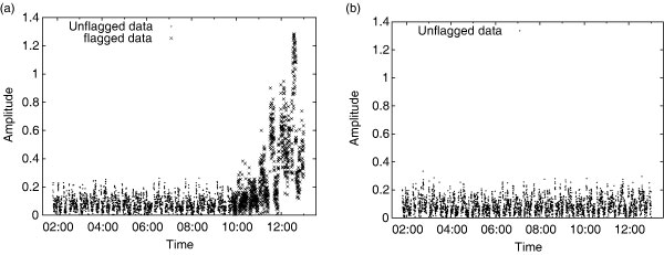
Figure 2 shows the effect of pieflag on data observed with the ATCA at L-band outside the spectral regions reserved for radio astronomy, between 1.38 GHz and 1.48 GHz. This band is particularly contaminated by RFI at the beginning and end of observations, when the antennae are pointed towards or away from the town of Narrabri, 20 km distant from the telescope.
Figure 3 shows data from the same observing run, but from a different frequency channel. The RFI in this channel has much higher amplitudes but is confined to very short periods of time. The Figure illustrates the effect of the second step of postprocessing.

|

|
Figure 4 shows data from an experiment in which the visibility amplitudes are dominated by the astronomical source, which has significant structure. Flagging based on amplitude did not work, since the cutoff was chosen such that much of the RFI at the beginning of the experiment was not detected. However, RMS-based flagging did find the affected data. This Figure also illustrates that a small amount of RFI in the reference channel has no noticeable effect on the flagging process.
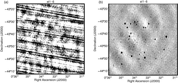
Figure 5 demonstrates the effect of pieflag on the final image.
|
Conclusions
pieflag can efficiently search interferometry data for man-made RFI. The implemented algorithms can deal with a variety of observational circumstances, are robust and find virtually all RFI-affected data which would be found by visual inspection. Usage of pieflag makes the flagging procedure much faster, relieves observers from an annoying part of the data calibration, and can easily be set up to run in data calibration scripts without any human interaction.
Ellingson,
S. W. 2004, ExA, 17, 261
An error has occurred in (ref id="R1").
Variable LPAGE is undefined. [empty string]
array
1
struct
COLUMN
0
ID
??
LINE
243
RAW_TRACE
at cfincludeJournalRef_B2ecfm1510229986._factor10(G:\www\publishha\app\views\journal\includeJournalRef_B.cfm:243)
TEMPLATE
G:\www\publishha\app\views\journal\includeJournalRef_B.cfm
TYPE
CFML
2
struct
COLUMN
0
ID
CF_INCLUDEJOURNALREF_B
LINE
180
RAW_TRACE
at cfincludeJournalRef_B2ecfm1510229986._factor12(G:\www\publishha\app\views\journal\includeJournalRef_B.cfm:180)
TEMPLATE
G:\www\publishha\app\views\journal\includeJournalRef_B.cfm
TYPE
CFML
3
struct
COLUMN
0
ID
CF_INCLUDEJOURNALREF_B
LINE
177
RAW_TRACE
at cfincludeJournalRef_B2ecfm1510229986._factor13(G:\www\publishha\app\views\journal\includeJournalRef_B.cfm:177)
TEMPLATE
G:\www\publishha\app\views\journal\includeJournalRef_B.cfm
TYPE
CFML
4
struct
COLUMN
0
ID
CF_INCLUDEJOURNALREF_B
LINE
176
RAW_TRACE
at cfincludeJournalRef_B2ecfm1510229986._factor14(G:\www\publishha\app\views\journal\includeJournalRef_B.cfm:176)
TEMPLATE
G:\www\publishha\app\views\journal\includeJournalRef_B.cfm
TYPE
CFML
5
struct
COLUMN
0
ID
CF_INCLUDEJOURNALREF_B
LINE
170
RAW_TRACE
at cfincludeJournalRef_B2ecfm1510229986._factor40(G:\www\publishha\app\views\journal\includeJournalRef_B.cfm:170)
TEMPLATE
G:\www\publishha\app\views\journal\includeJournalRef_B.cfm
TYPE
CFML
6
struct
COLUMN
0
ID
CF_INCLUDEJOURNALREF_B
LINE
15
RAW_TRACE
at cfincludeJournalRef_B2ecfm1510229986._factor41(G:\www\publishha\app\views\journal\includeJournalRef_B.cfm:15)
TEMPLATE
G:\www\publishha\app\views\journal\includeJournalRef_B.cfm
TYPE
CFML
7
struct
COLUMN
0
ID
CF_INCLUDEJOURNALREF_B
LINE
12
RAW_TRACE
at cfincludeJournalRef_B2ecfm1510229986._factor42(G:\www\publishha\app\views\journal\includeJournalRef_B.cfm:12)
TEMPLATE
G:\www\publishha\app\views\journal\includeJournalRef_B.cfm
TYPE
CFML
8
struct
COLUMN
0
ID
CF_INCLUDEJOURNALREF_B
LINE
11
RAW_TRACE
at cfincludeJournalRef_B2ecfm1510229986._factor43(G:\www\publishha\app\views\journal\includeJournalRef_B.cfm:11)
TEMPLATE
G:\www\publishha\app\views\journal\includeJournalRef_B.cfm
TYPE
CFML
9
struct
COLUMN
0
ID
CF_INCLUDEJOURNALREF_B
LINE
1
RAW_TRACE
at cfincludeJournalRef_B2ecfm1510229986.runPage(G:\www\publishha\app\views\journal\includeJournalRef_B.cfm:1)
TEMPLATE
G:\www\publishha\app\views\journal\includeJournalRef_B.cfm
TYPE
CFML
10
struct
COLUMN
0
ID
CFINCLUDE
LINE
3230
RAW_TRACE
at cfArticle2ecfc1291681887$funcREFERENCESDTD1._factor150(G:\www\publishha\app\modules\journal\Article.cfc:3230)
TEMPLATE
G:\www\publishha\app\modules\journal\Article.cfc
TYPE
CFML
11
struct
COLUMN
0
ID
CF_ARTICLE
LINE
3217
RAW_TRACE
at cfArticle2ecfc1291681887$funcREFERENCESDTD1._factor151(G:\www\publishha\app\modules\journal\Article.cfc:3217)
TEMPLATE
G:\www\publishha\app\modules\journal\Article.cfc
TYPE
CFML
12
struct
COLUMN
0
ID
CF_ARTICLE
LINE
3216
RAW_TRACE
at cfArticle2ecfc1291681887$funcREFERENCESDTD1.runFunction(G:\www\publishha\app\modules\journal\Article.cfc:3216)
TEMPLATE
G:\www\publishha\app\modules\journal\Article.cfc
TYPE
CFML
13
struct
COLUMN
0
ID
CF_TEMPLATEPROXY
LINE
2938
RAW_TRACE
at cfArticle2ecfc1291681887$funcBACKSECTIONSDTD1.runFunction(G:\www\publishha\app\modules\journal\Article.cfc:2938)
TEMPLATE
G:\www\publishha\app\modules\journal\Article.cfc
TYPE
CFML
14
struct
COLUMN
0
ID
CF_TEMPLATEPROXY
LINE
146
RAW_TRACE
at cfgenArticleContent2ecfm782833447._factor5(G:\www\publishha\app\views\journal\generator\genArticleContent.cfm:146)
TEMPLATE
G:\www\publishha\app\views\journal\generator\genArticleContent.cfm
TYPE
CFML
15
struct
COLUMN
0
ID
CF_GENARTICLECONTENT
LINE
1
RAW_TRACE
at cfgenArticleContent2ecfm782833447._factor6(G:\www\publishha\app\views\journal\generator\genArticleContent.cfm:1)
TEMPLATE
G:\www\publishha\app\views\journal\generator\genArticleContent.cfm
TYPE
CFML
16
struct
COLUMN
0
ID
CF_GENARTICLECONTENT
LINE
1
RAW_TRACE
at cfgenArticleContent2ecfm782833447.runPage(G:\www\publishha\app\views\journal\generator\genArticleContent.cfm:1)
TEMPLATE
G:\www\publishha\app\views\journal\generator\genArticleContent.cfm
TYPE
CFML
17
struct
COLUMN
0
ID
CFINCLUDE
LINE
10
RAW_TRACE
at cfStaticPageLayout2ecfm1426351739.runPage(G:\www\publishha\app\views\layout\StaticPageLayout.cfm:10)
TEMPLATE
G:\www\publishha\app\views\layout\StaticPageLayout.cfm
TYPE
CFML
18
struct
COLUMN
0
ID
CFINCLUDE
LINE
30
RAW_TRACE
at cfCacheController2ecfc639388092$funcRENDERLAYOUT.runFunction(G:\www\publishha\app\controller\CacheController.cfc:30)
TEMPLATE
G:\www\publishha\app\controller\CacheController.cfc
TYPE
CFML
19
struct
COLUMN
0
ID
CF_UDFMETHOD
LINE
241
RAW_TRACE
at cfCacheController2ecfc639388092$funcGENARTICLECONTENT.runFunction(G:\www\publishha\app\controller\CacheController.cfc:241)
TEMPLATE
G:\www\publishha\app\controller\CacheController.cfc
TYPE
CFML
20
struct
COLUMN
0
ID
CF_UDFMETHOD
LINE
327
RAW_TRACE
at cfCacheController2ecfc639388092$funcGENARTICLE.runFunction(G:\www\publishha\app\controller\CacheController.cfc:327)
TEMPLATE
G:\www\publishha\app\controller\CacheController.cfc
TYPE
CFML
21
struct
COLUMN
0
ID
CF_UDFMETHOD
LINE
39
RAW_TRACE
at cfCacheController2ecfc639388092$funcGENCACHE.runFunction(G:\www\publishha\app\controller\CacheController.cfc:39)
TEMPLATE
G:\www\publishha\app\controller\CacheController.cfc
TYPE
CFML
22
struct
COLUMN
0
ID
CF_CFPAGE
LINE
634
RAW_TRACE
at cfPublishingApp2ecfc536529069$funcPROCESSREQUEST.runFunction(G:\www\publishha\app\PublishingApp.cfc:634)
TEMPLATE
G:\www\publishha\app\PublishingApp.cfc
TYPE
CFML
23
struct
COLUMN
0
ID
CF_TEMPLATEPROXY
LINE
16
RAW_TRACE
at cfBootstrap2ecfc660975501$funcHANDLEREQUEST.runFunction(G:\www\publishha\app\Bootstrap.cfc:16)
TEMPLATE
G:\www\publishha\app\Bootstrap.cfc
TYPE
CFML
24
struct
COLUMN
0
ID
CF_TEMPLATEPROXY
LINE
18
RAW_TRACE
at cfApplication2ecfc757760907$funcONREQUESTSTART.runFunction(G:\www\publishha\webroot\Application.cfc:18)
TEMPLATE
G:\www\publishha\webroot\Application.cfc
TYPE
CFML
1 www.astron.nl/~renting/flagger.html
2 The original name of the program, ‘pyflag’, turned out to be already in use, requiring a name modification of some sort to avoid confusion.
3 www.narrabri.atnf.csiro.au/observing/rfi/
4 www.atnf.csiro.au/people/Enno.Middelberg/pieflag