

Cosmological Surveys with the Australian Square Kilometre Array Pathfinder
A. R. Duffy A C , A. Moss B and L. Staveley-Smith AA ICRAR, The University of Western Australia, M468, 35 Stirling Hwy, WA 6009, Australia
B Department of Physics and Astronomy, University of British Columbia, 6224 Agricultural Road, Vancouver, BC, V6T 1Z1, Canada
C Corresponding author. Email: alan.duffy@icrar.org
Publications of the Astronomical Society of Australia 29(2) 202-211 https://doi.org/10.1071/AS11013
Submitted: 21 March 2011 Accepted: 21 March 2012 Published: 3 May 2012
Journal Compilation © Astronomical Society of Australia 2012
Abstract
This is a design study into the capabilities of the Australian Square Kilometre Array Pathfinder in performing a full-sky low redshift neutral hydrogen survey, termed WALLABY, and the potential cosmological constraints one can attain from measurement of the galaxy power spectrum. We find that the full sky survey will likely attain 6 × 10⁵ redshifts which, when combined with expected Planck CMB data, will constrain the Dark Energy equation of state to 20%, representing a coming of age for radio observations in creating cosmological constraints.
Keywords: (cosmology): cosmological parameters — galaxies: statistics — methods: numerical — radio lines: galaxies — telescopes
1 Introduction
With the advent of large cosmological volume galaxy surveys, comprised of well measured positional information from homogenous datasets, the measurement of the galaxy matter power spectrum has become almost routine. The use of such power spectra in the determination of the cosmological model has been based almost exclusively, however, on optical techniques, e.g. the 2dF Galaxy Redshift Survey (2dFGRS1) and the Sloan Digital Sky Survey (SDSS2). The overall shape of the power spectrum is sensitive to the cosmological parameter constraints Γ = Ωm h and fb = Ωb/Ωm, where Ωm and Ωb are the total matter and baryon densities defined relative to critical, and h = H0/(100 km s–1 Mpc–1), as well as the spectral index of the density fluctuations, ns, and neutrino densities (e.g. Percival et al. 2001; Tegmark et al. 2004a,b; Cole et al. 2005; Abdalla and Rawlings 2007). Additional information from the power spectrum can be gleaned by measuring the physical scale of the so-called Baryonic Acoustic Oscillations (e.g. Blake & Glazebrook 2003; Percival et al. 2010) either through using the scale as a ‘standard ruler’ or by combining with measurement of the Cosmic Microwave Background to break degeneracies. These measurements allow the determination of the nature of the Dark Energy, through constraining the equation of state parameter, w, which for the cosmological constant is –1. With enough sufficiently distant galaxies the variation of the equation of state parameter with redshift can be constrained by comparing this acoustic scale in different epochs, as considered in, e.g. Abdalla, Blake & Rawlings (2010).
Recent advances of the speed at which radio telescopes can survey the sky to a given flux limit point to the possibility of radio joining optical surveys to measure the matter power spectrum. The distribution of these sources along the line of sight is accurately determined by using the redshifted emission line at ≈21 cm of the hyperfine splitting transition in neutral hydrogen (Hi). Previously surveys have been limited to ~103 galaxies (e.g. Zwaan et al. 2005; Lang et al. 2003) whilst the very latest Hi catalogue from the Arecibo legacy survey, ALFALFA, is expected to find ~104 objects (Giovanelli et al. 2005). In the near future the Chinese-built Five-hundred Aperture Spherical Telescope (Nan 2006) could detect as many as ~106 in the current design (Duffy et al. 2008). Ultimately however, the future for radio galaxy surveys is the Square Kilometre Array, SKA,3 which may detect ~109 galaxies (Abdalla and Rawlings 2005). The initial step towards the SKA facility is a precursor known as the Australian SKA Pathfinder or ASKAP.4 The pathfinder consists of a much reduced number of telescopes, but still operating with a large Field of View (FoV) of the sky, which therefore enables the revolutionary upgrade in survey speed.
The low-redshift precursor surveys of the SKA will accurately measure the properties of galaxies at low redshift and how these properties change as a function of environment, for example what is the dependence of the Hi mass function on local galaxy density? The deeper precursor surveys will measure evolutionary effects. In this work we will demonstrate that simple estimates of the number and distribution of Hi detected galaxies will enable ASKAP to be the first radio telescope to derive cosmological parameter constraints, able to constrain the Dark Energy equation of state to 20%. This is a similar capability to previous optically based measurements such as with 2dF (Cole et al. 2005) but significantly more collecting area will be needed to rival current optical surveys such the 6dF (Beutler et al. 2011), SDSS II luminous red galaxy survey (e.g. Thomas, Abdalla & Lahav 2011) and WiggleZ (Blake et al. 2010) surveys much less forthcoming optical surveys such as the SDSS III Baryon Oscillation Spectroscopic Survey (BOSS5). However we note that future radio surveys with, for example, the SKA have the capability to exceed the volume and numbers of galaxies spectroscopically detected compared with optical surveys.
While limiting our study to the use of the power spectrum in constraining cosmology (e.g. Blake & Glazebrook 2003) we note that the spectroscopic nature of radio surveys enable other cosmological probes. One such use is in measuring redshift-space distortions, a statistical measurement of infalling galaxies near large scale structure, which can probe the growth of structure on cosmic scales and hence providing a strong test of the validity of General Relativity as well as Dark Energy models (e.g. Song & Percival 2009; Blake et al. 2010) over ~Mpc scales. With a relatively high density of galaxies probing a given volume WALLABY will likely equal, if not exceed, constraints on this measurement by an optical survey such as 6dF (Beutler et al., in prep). Instead of using the redshifts one can calculate the distance to the galaxies themselves, using relations such as the Tully-Fisher (Tully & Fisher 1977) or Fundamental Plane (Faber et al. 1987; Djorgovski & Davis 1987), to estimate the Hubble flow which can then be removed to leave the peculiar velocities of each galaxy. These velocities form a velocity field, or Bulk Flow, that reflects the matter distribution, allowing constraints of the amount of mass and the fluctuation of overdensities in the Universe (e.g. Burkey & Taylor 2004; Abate et al. 2008; Watkins, Feldman & Hudson 2009).
We detail the techniques and assumptions considered in our calculation of galaxy detections in Section 2, in particular the effect of telescope resolution and galaxy inclinations in limiting galaxy counts (Section 2.3). Utilising these assumptions we calculate the expected number of galaxies that the all-sky ASKAP (WALLABY) survey could be expected to find in Section 3. By constraining the matter power spectrum we then estimate the suitability of the WALLABY survey as a cosmological probe in Section 4.
2 Method
We have utilised a, significantly, updated methodology to Duffy et al. (2008) which analysed the potential galaxy surveying power of the Five hundred metre Aperture Spherical Telescope (FAST). Therefore the reader may wish to consult that article for a more in-depth discussion on the following issues, including a consideration of evolution in the Hi mass function (WALLABY is a shallow survey and hence likely to be unaffected by evolution). However there is one significant difference between FAST and ASKAP, namely that the former is a single dish and the latter an interferometer. A difference that potentially has significant effects in terms of resolving out extended structure. As we shall see the loss of signal from this effect is an issue for objects at all redshifts not just those closest to the observer (and hence with the largest angular extent on the sky). In other words, with the large baselines, 2 km, available to WALLABY, most detections are resolved and hence one must consider this issue. The positive counterpoint to this high resolution is that the galaxies rarely overlap within the beam of the telescope and the survey is effectively never confusion limited, as discussed in Section 2.2.
For an interferometer observing a resolved structure one can attempt to recover some (but not all) of the missing flux by smoothing the data, i.e. spatially integrating. However, some flux will be lost as spatial smoothing is akin to removing the longer antenna baseline pairs and therefore results in a loss of sensitivity. Exact characterisation of the effect depends in detail on the distribution of neutral hydrogen in each galaxy and the properties of the ‘source finder’. This is a complex issue and a detailed discussion of angular size distributions of detected galaxies is therefore deferred to a later paper (Duffy et al., in prep). However, a simple approximation is that, if there are n independent pixels (beams) that make up a galaxy (where we use the example n >> 1), the S/N ratio of those pixels, when combined, will be improved by  if the object is approximated by a top hat column density and velocity profile. We consider this effect in more detail in Section 2.3 and find that there is a non-negligible reduction in the galaxy counts of order 20% if one considers a reduction in S/N due to this effect.
2.1 Estimating the Hi Signal
As detailed in Duffy et al. (2008) and references therein, the expected thermal noise for a dual polarisation, npol = 2, single beam is given by
for an observing time of t and a frequency bandwidth Δν, where k = 1380 Jy m2 K–1 is the Boltzmann constant and Tsys is the system temperature (assumed to be 50 K). The effective area, Aeff, calculation has been modified from the previous single dish calculation to better reflect the interferometric nature of ASKAP. The individual effective area of an ASKAP dish is the geometric area of a 12-m diameter dish, aeff, reduced by the aperture efficiency, expected to be αeff ≈ 0.8 (Johnston et al. 2008). Due to computational limitations in correlating signals from all 36 dishes in ASKAP, WALLABY will likely use the inner core of 30 dishes, Ndish = 30, which can be combined in Nperm = Ndish(Ndish – 1)/2 permutations. The resolution of the inner core is limited to 30″ at the 21-cm wavelength using the central 2 km baselines of ASKAP. For each pairwise correlation we assume a  boost to the signal-to-noise by averaging the real and imaginary signal from a complex correlator (Thompson 2007). This leads to an overall effective area for ASKAP of
where we have averaged over the complex and real signals.
Typically, the beam area increases like  which, if one uniformly tiles the z = 0 sky, has the positive result that slices at higher redshift receive extra exposure due to the fact that observations will overlap. This reduces the flux limit relevant to a particular redshift slice by a factor
  , as discussed by Abdalla and Rawlings (2005). This is not the case for ASKAP however, as the number of on sky beams varies as a function of frequency to ensure that there is an approximately fixed covering area as a function of redshift. Hence, the flux limit for an observation, Slim, for a specific signal-to-noise ratio (S/N) is given by

We relate this flux to the Hi mass, MHi, of a galaxy at redshift z in terms of the observed flux, S, and line width, ΔVo, by Roberts (1975)
where dL(z) is the luminosity distance to the galaxy, necessitating the  correction for an FRW universe. In a significant departure from the methodology of Duffy et al. (2008) we make use of the measured number density of objects as a function of velocity widths and Hi masses directly from HIPASS, presented in Zwaan, Meyer & Staveley-Smith (2010). With this method we automatically include the effects of angle of inclinations of galaxies as well as the complex velocity-structure of the system.
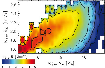
In Figure 1 we show the full matrix utilised noting that the histogram widths are 0.01 dex whereas the colour scheme is the standard number density in decades of mass and velocity. We emphasise that this represents the very latest information pertaining to the frequency of Hi systems as a function of mass and velocity widths and, due to the limited redshift surveyed by WALLABY, is an ideal basis for estimating galaxy number counts.
|
To explicitly incorporate the matrix information we must recast Equation 4, first dividing by ΔVo (the ratio is termed a peak flux Speak ≡ MHi/ΔVo, implicitly assuming the galaxy spectral profile is a top-hat). This means that for each grid cell in Figure 1 we can also divide the Hi mass by the velocity width (W20 is assumed to be the full velocity width of the system) and read off the number density of galaxies in those cells which lie above this peak flux. To determine what the minimum observable flux is (as a function of redshift) we substitute the flux limit of the survey (Equation 3) for S in Equation 4 allowing us to create the following inequality to determine when a population of Hi sources will be detected by ASKAP
where Nch is the number of channels that the galaxy will be distributed across, calculated as rounding to the nearest integer number of channel ΔVo/dV (where dV in ASKAP is 4 km s–1) in a calculation similar to Equation 8 of Rawlings (2004).
One can estimate the number of galaxies detected in the survey by adding the densities of all populations that fulfil the inequality in Equation 5 with a peak flux Slimpeak(z) by computing
where the sky area covered is ΔΩ and the size of the redshift bin is Δz, dV/dzdΩ is the comoving volume element for the FRW universe and dN/dVdSpeak ≡ dN/dV(dMHi/dW20) is the comoving number density of galaxies per unit peak flux, taken from the matrix of Figure 1. No evolution in the Hi mass-velocity width space has been assumed over the limited redshift surveyed in WALLABY, nor is there any apparent evolution in the integrated cosmic Hi density out to z ≈ 0.8 (Chang 2010) or indeed z ≈ 2 (Prochaska, O’Meara & Worseck 2010). We calculate the average redshift of galaxies in the survey from N(Speak > Slimpeak, z) by integrating appropriately over z, that is,
2.2 Confusion of Galaxies
A limiting factor in galaxy surveys is the issue of confusion, whereby detections in Hi are unable to be unambiguously assigned to a single galaxy. Typically Hi surveys have previously had far greater discrimination between objects along the line of sight than in the plane of the sky. ASKAP will differ in this regard by enabling wide-field surveys of the sky with at least 30-arcsec resolution (ASKAP baselines of 2 km) together with highly competitive 4 km s–1 velocity resolution. It is therefore unlikely that confusion will play a significant role in limiting the number of galaxy detections in the WALLABY survey, an expectation we verify by making use of a simple analytic estimate of the expected level of confusion (as given in Staveley-Smith 2008).
To estimate the confusion rates one must have a measure of how many galaxies are in the survey volume, which we estimate from the Hi mass function as measured by Zwaan et al. (2005),
where α = –1.37,  = 1.42 × 10⁻² (h–1 Mpc)–3 and M
 = 109.8 M⊙. The number density of galaxies, n0, with a mass larger than Mlim is given by the integral of this Schechter function resulting in the well known Γ function:
The total Hi mass contained in systems above Mlim is given by the mass weighted integral of the Schechter function
We are interested in understanding the confusion rates with sources that would significantly contribute to the mass of the main detection. Using Equation 10 we can evaluate the Hi mass fraction contained in sources above a limiting mass; only 21% of the Hi in the Universe is contained in systems of mass greater than M , while 75% of the mass is contained within systems more massive than 0.1M
 . To a good approximation therefore we can calculate confusion rates from sources of this mass and greater. The typical density of sources above 0.1M
 is found using Equation 9, which for the Hi mass function of Zwaan et al. (2005) is 0.017 Mpc–3.
We then calculate the typical distribution of the galaxies on the sky, as given by the galaxy-galaxy distribution which relates the typical density of sources n0 as a function of comoving distance r from a given galaxy, approximated in the non-linear regime by
where r0 is the correlation length. The average number of objects in a cylinder of comoving line-of-sight depth, β, and transverse comoving radius, κ, is
For  the solution is
where 2F1 is a hypergeometric function. Assuming, reasonably, that the distribution of galaxies does not evolve over the redshift range probed by WALLABY we can make use of the HIPASS galaxy–galaxy correlation function measurements of Meyer et al. (2007) (γ = –1.5 and r0 = 4.7 Mpc). The cylinder diameter, 2κ, is set by the ASKAP beam. For the natural Gaussian antenna distributions described in Staveley-Smith (2006) and modelled in Gupta, Johnston & Feain (2008) the Full-Width Half Maximum beam extent for WALLABY is

where we have conservatively assumed that the maximum ASKAP baseline is 2 km. The cylinder depth is set by the accuracy of the available redshifts for the confusing population, Δz.
Although the 4 km s–1 velocity width of ASKAP will ensure that the spectroscopic redshifts of WALLABY will be measured to approximately 10–5 the best spectroscopic redshift estimate in practice will be limited by the typical Doppler width of the galaxy. If we assume, conservatively, that two M galaxies of typical velocity width 300 km s–1 are just overlapping then Δz = 600 km s–1/c = 0.002. Even with this conservative calculation the chances that there will be more than one galaxy in the beam volume, i.e. the confusion rate, is at a negligible sub-percent level for the mean redshift of the survey z ≈ 0.05 (determined in Section 3) where the majority of detections lie. However, as one surveys deeper in the Universe the confusion rate will steadily increase as the telescope beam encompasses greater regions of space, further compounded by the lengthening observed wavelength, yet even at the survey edge of WALLABY, z = 0.26 we find that less than 5% of galaxies will be confused.
Using this formalism we can also calculate the typical success rates in assigning an optical counterpart to the Hi detected galaxies, assuming that such an optical catalogue contains all these Hi galaxies we can then utilise the same number density as before. As a worst case scenario we further assume that only optical photometric redshifts are available, with a ‘typical’ redshift error Δz ≈ 0.05 (Hildebrandt et al. 2008). Thus the chances that we can unambiguously assign an optical counterpart (i.e. there is only one galaxy in the volume) occurs in more than 97% of cases at the average redshift of the WALLABY survey z ≈ 0.05 (determined in Section 3). At the survey edge the success rate is 80% which is more than acceptable for most science cases. However, this value is a conservative case as we could blindly assign a counterpart from the candidates, i.e. if there were two galaxies in the beam volume then we would be right 50% of the time. This could be further improved by using prior knowledge and choosing the largest stellar counterpart, for example.
In conclusion, provided ASKAP baselines of 2 km are available (i.e. the most conservative case) the overall galaxy number counts will be largely unaffected by confusion and this effect is henceforth ignored in the following discussion. To enable unambiguous optical counterparts detections for the majority of ASKAP Hi detections we find that photometric errors of order Δz ≈ 0.05 are sufficient unless surveys probe deeper in redshift (by z ≈ 0.4 the success rate is less than 50%) or precise redshifts are needed, for example if attempting spectral stacking experiments, in which case a spectroscopic follow up in the optical is demanded.
2.3 Resolving Rotating Galaxies
An important consideration for interferometers is the issue of resolving out galaxies that are larger in extent than the beamsize. For ASKAP, with a 2-km baseline this will certainly be an issue for extended sources. Furthermore with 4- km s–1 velocity resolution ASKAP will also probe the velocity structure of the galaxies themselves hence we try to estimate the size, inclination and typical rotation velocities of the galaxies that are present in the Hi mass-velocity matrix.
We estimate the angle of inclination, θ, of the galaxy by relating the measured velocity width ΔVo from the Hi-mass-velocity matrix, to the intrinsic linewidth width, ΔVe. The difference between the true velocity and observed velocities is proportional to sin(θ). We can use the Hi mass from the Hi mass-velocity matrix to determine the intrinsic linewidth of a galaxy, corrected for broadening, using the empirical relation found by (Briggs & Rao 1993; Lang et al. 2003) to be
although we note that this relation shows a large dispersion, especially for dwarf galaxies. The linewidth of a galaxy, ΔVθ, which subtends an angle θ between its spin axis and the line-of-sight can be computed using the Tully-Fouque rotation scheme (Tully & Fouque 1985):
ΔVc = 120 km s–1 represents an intermediate transition between the small galaxies with Gaussian Hi profiles in which the velocity contributions add quadratically and giant galaxies with a ‘boxy’ profile reproduced by the linear addition of the velocity terms. ΔVt ≈ 20 km s–1 is the velocity width due to random motions in the disk (Rhee & van Albada 1996; Verheijen & Sancisi 2001).
With this definition of θ, zero corresponds to face-on and  to edge-on. In cases where
  , one can see that
  . For θ = 0, one finds that
  , in other words the Hi dispersion in the disk, whereas for
  we recover
  as expected.
In addition there is a broadening effect,  , of the Hi profile due to the frequency resolution of the instrument, R. For a range of galaxy profiles, this broadening is found to be ΔVinst ≈ 0.55R (Bottinelli et al. 1990). As befits a next generation ratio instrument the ASKAP velocity width is extremely fine, ΔVinst ≈ 4 km s–1, which is an insignificant source of error in the present discussion.
However, for completeness we add ΔVinst linearly to ΔVθ, as argued by Lang et al. (2003), to give the effective observed linewidth,

The inclination angle θ can be solved for in Equation 16 by substituting the above effective observed linewidth (Equation 17) and the intrinsic linewidth from Equation 15. We note that calculating the angle of inclination from the matrix presented in Figure 1 in this way finds less galaxies than by randomly assigning an angle of inclination, uniform in cosine, to the galaxies (which typically raises the completeness for WALLABY to 90%), in this case the more detailed calculation is the more conservative estimate.
To determine the extent of an object on the sky, and hence ultimately the number of beams that resolve the structure, we make use of an empirically derived relation between the Hi mass of a galaxy and the Hi diameter, DHi (defined to be the region inside which the Hi surface density is greater than 1 M⊙ pc–2). From Broeils & Rhee (1997); Verheijen & Sancisi (2001) we have
The on-sky area of the galaxy can then be estimated (Meyer et al. 2008) using π(DHi/2)2 (B/A)2 where A and B are the major and minor axes respectively, the ratio of which (B/A) is equal to cos(θ) which is calculated above. In practice we limit the smallest measurable angle of inclination for spirals to  in accordance with Masters, Giovanelli & Haynes (2003). We compare the apparent area of the galaxy on the sky, scaling by the square of the angular diameter distance dA(z), with the assumed Gaussian beam of ASKAP, Abeam, given by
where ΩFWHM was defined in Equation 14 previously.
As described at the start of Section 2 we assume that the Signal-to-Noise of the galaxy is reduced when we are forced to recombine the multiple beams by which a galaxy is, potentially, resolved. The loss of signal is approximated by the square root of the number of beams needed to cover a given galaxy, given by the galaxy area, Agal, divided by the beam area, Abeam. In practice the beam and galaxy widths are convolved when estimating this reduction, ensuring that even if the galaxy matches the beam size an additional factor of unity is added to this number of beams, giving a  reduction in signal in this case. Hence we reduce the peak flux Speak in the detection Equation 5 by this geometric factor
  . For the current design of WALLABY, with a 2 km baseline, nearly 80% of all galaxies are recovered after this reduction in peak flux.
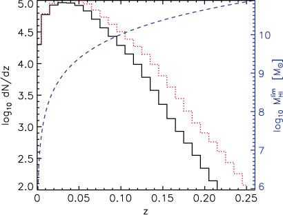
In Figure 2 we compare the predicted number counts as a function of redshift for the full sky WALLABY survey both with (black, solid curve) and without (red, dot curve) the effects of resolving the galaxies. Clearly this effect is particularly an issue for the faint distant sources which are both face-on and massive to be resolved out.
|
3 Galaxy Survey
In this section we combine our estimates of the detectability of galaxies from the previous section, with the ASKAP strawman figures (Johnston et al. 2008) and the specifics of the WALLABY survey (Koribalski & Staveley-Smith 2008), as in Table 1.
|
Table 1 summarises the survey specific values of WALLABY (Koribalski & Staveley-Smith 2008) in addition to the strawman values of ASKAP (Johnston et al. 2008). We consider the reduced baseline model for WALLABY which utilises the inner 30 dishes across a maximum 2-km baseline rather than the full 36-dish, 6-km extent of ASKAP. We also have two numbers for the predicted galaxy counts, and their mean redshift, reflecting the effects of including the reduction of signal-to-noise by spatially resolved galaxies, as demonstrated in Figure 2. The brackets ignore this effect and hence have a larger galaxy count. We consider the conservative estimate for ASKAP when noting the effective volume, as given in Equation 25, for the typical k-mode of interest (roughly the position of the first Baryonic Acoustic Oscillation peak). We also give the estimated percentage measurement error of the power spectrum at this scale. The maximum redshift we can probe the first peak out to, with nP = 3, is z = 0.116 with a number density of sources estimated at n = 1.07 × 10⁻⁴ Mpc–3. At the second peak k = 0.125 h–1 Mpc we find the effective volume to be 3.6 × 10⁷ Mpc3 and σP/P = 7%.
In Figure 2 the dashed blue curve indicates the expected neutral hydrogen mass limit as a function of redshift in redshift bins of width Δz = 0.01 for a single pointing of ASKAP. The redshift depth of WALLABY is such that the survey ends when the mass limit approaches ≤1011 M⊙, which is the apparent maximal limit of Hi systems.
The expected number counts as a function of redshift on completion of the proposed survey is shown in Figure 2 as the solid black curve with the actual total number of detections and mean redshift of WALLABY given in Table 1.
4 Cosmological Parameters
Using the predicted galaxy number counts for WALLABY we can estimate the errors on the galaxy power spectrum at the mean redshift of the survey z = ![]() z
z![]() ≈ 0.055 and ultimately the expected constrains on cosmological parameters. P(k, z) is related to the power spectrum P(k, 0) by
≈ 0.055 and ultimately the expected constrains on cosmological parameters. P(k, z) is related to the power spectrum P(k, 0) by

where b is the bias parameter and D(z) is the growth factor computed6 from
where E(z) = H(z)/H0 and by construction D(z = 0) = 1.
Errors on the power spectrum are due to two factors: sample variance, i.e. the fact that not all k modes are measured, and shot-noise, which is the effective noise on the measurement of an individual mode. The total error σP on the measurement of the power spectrum, P(k, z), for a given k with bin width Δk can be expressed as (Feldman, Kaiser & Peacock 1994; Tegmark 1997; Blake et al. 2006)
where P = P(k, z) and
is the number density of galaxies which are detected (making nP dimensionless) and m is the number of k-modes in a survey of total volume V, with m = 2πk2 Δk V/(2π)3. The ability of a survey to probe cosmological parameters can be estimated, and compared, with the effective survey volume Veff given by
As argued by Seo and Eisenstein (2003) there is no great gain in probing beyond nP = 3 hence we limit the volume of our survey to a maximum redshift zmax when n(z = zmax)P(k) = 3; conservatively assuming a constant number density within this volume, hence the effective volume is now evaluated as
evaluated in Table 1 for two k-modes of interest (k = 0.065 and 0.125 h–1Mpc–1), approximately corresponding to the baryonic peaks in the power spectrum. Note that we have assumed a constant weighting function for the galaxies used in the power spectrum measurement, a so-called ‘number-weighting’ scheme. With our assumptions of constant number density within a given maximum redshift the WALLABY survey is essentially a uniform survey (i.e. with a window function which is effectively the identity matrix) and the covariance matrix of the k-bands can be well represented by a diagonal covariance matrix with elements equal to (4/3)2(P2/m) as argued in Blake et al. (2006).
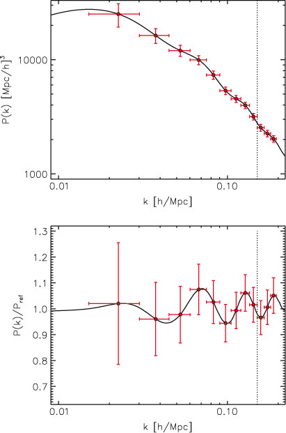
In this work we create a power spectrum (Lewis, Challinor & Lasenby 2000) based on the latest WMAP7 Maximum Likelihood cosmology (Komatsu et al. 2009) for the standard ΛCDM model with values [Ωb, Ωm, Ω∧, h, w, ns, σ8] given by [0.0451, 0.271, 0.729, 0.703, –1, 0.966, 0.809]. In the top panel of Figure 3 we demonstrate the power spectrum with the expected errors from WALLABY. In the bottom panel of this figure we have normalised the matter power spectrum by a reference no-oscillation power spectrum (Eisenstein & Hu 1998) to aid visualisation of the peaks. It appears that with the errors from WALLABY it will be challenging to identify the ‘baryonic wiggles’. To quantify this we have performed a χ2 test on the no-oscillation model with the datapoints in Figure 3 to determine if the datapoints have sufficiently small errorbars to rule out this wiggle-less model. The χ2/d.o.f value is 2.2/7, this means that WALLABY will only detect the BAO peaks with  significance. Although not conclusive this analysis does suggest that WALLABY will not significantly detect the Baryonic Acoustic Oscillations (BAO), therefore we do not attempt to use these oscillations as standard rulers.7
|
In accordance with our previous method of the analysis of FAST (Duffy et al. 2008) we limit our investigation of the power spectrum to band-powers over the range 0.005 < k/h Mpc–1 < 0.15. The maximum wavenumber chosen is a conservative cut on the power spectrum to ensure that we perform our analysis in the linear regime (as suggested in Cole et al. 2005). It has been suggested (Beutler et al., in prep) that an Hi survey such as WALLABY could safely trace even smaller scales (~0.2 h Mpc–1). This is because of the inherent low bias of Hi detections which are tidally stripped in high-density regions, hence a blind Hi survey will naturally avoid these regions, ensuring that the nonlinear effects due to peculiar velocities of galaxies in these groups and clusters will be lessened, effectively extending the linear regime to smaller scales. For the Cosmic Microwave Background (CMB) data we have assumed that we have full polarisation information for Planck by considering the temperature T and E-type polarisation anisotropies for l < 2400 (including cross spectra), and assumed that they are statistically isotropic and Gaussian. The noise in the CMB data is also assumed to be isotropic and is based on a simplified model with NTt = NEe/4 = 2 × 10⁻⁴ μK2, having a Gaussian beam of 7 arcminutes (Planck Collaboration 2006). In the Markov–Chain Monte Carlo analysis we analytically marginalise over the bias parameter b in Equation 20 and assume that the priors around each cosmological parameter are flat, with a width safely outside that allowed by WMAP (Komatsu et al. 2009).
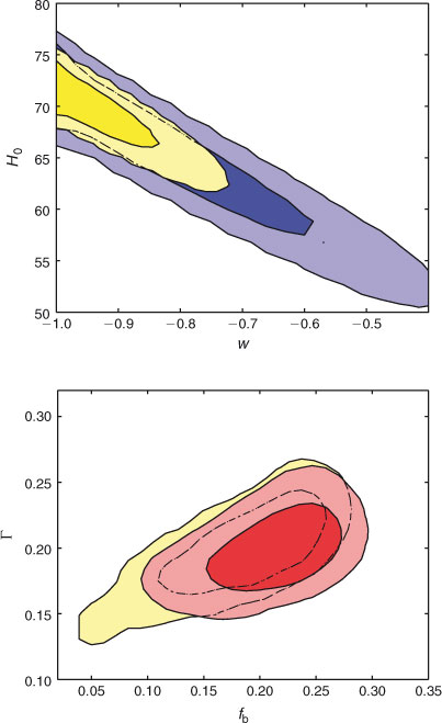
The values shown in Table 2 are best-fit cosmological values (Lewis & Bridle 2002) for a variety of different parameters using expected Planck CMB data alone and then combined with WALLABY (or 2dF as a comparison). Shown are the predicted cosmological parameter estimates when projected Planck CMB data is used alone, then in combination with WALLABY and also when used with an existing optical survey 2dF. Including the matter power spectrum measurements results in a factor two improvement in the constraints on the Dark Energy equation of state parameter w and the Hubble constant H0. Note that we performed a 6 parameter cosmological fit but that Planck has such small errors on most parameters that a survey with less than a few 106 sources is unlikely to improve the estimates, with the exception of w and H0, and for completeness we list the other variables which were unchanged when 2dF or WALLABY surveys were included; [ ,
,  , ns, log(1010As), τ] were constrained to be [0.0227 ± 0.0002, 0.1099 ± 0.0015, 0.964 ± 0.005, 3.06 ± 0.01, 0.092 ± 0.006].
|
By combining CMB data with the matter power spectrum measurement, which itself isn't a function of w, we break the degeneracy between w and h that occurs when calculating the distance to the surface of last scattering from the CMB. Thus the main effect of ASKAP is to reduce the error on h and w by a factor two on the value achieved with Planck alone, as demonstrated in the top panel of Figure 4. In the bottom panel of Figure 4 we compare WALLABY with an existing optical based measurement of the matter power spectrum from 2dF, the two error ellipses are of similar size, graphically illustrating the parameter estimates in Table 2 that WALLABY will be the first radio telescope to infer cosmological parameters from the matter power spectrum.
|
5 Conclusion
As is clear from the galaxy survey estimates for WALLABY, ASKAP will likely be the first radio telescope to measure the matter power spectrum, constraining cosmological parameters to the level attained by the optical survey 2dF in 2005, this will represent a coming of age for radio astronomy. To match, and ultimately surpass, current surveys such as WiggleZ will demand the full version of the SKA. In creating a radio based galaxy survey the matter power spectrum will be analysed using a different galaxy tracer together with different survey selection effects than the 2dF spectroscopic optical catalogue. Although not considered here there is the additional possibility of using the velocity field of the galaxies to gain additional cosmological constraints. As regards to a full local sample of ≈ 6 × 10⁵ Hi detected galaxies the science case is intriguing for the determination of star formation in the local Universe. When coupled with deeper surveys on ASKAP, such as DINGO, that can determine the evolution in redshift out to z = 0.4, the combined output will be a significant dataset for years to come.
Acknowledgments
The matter power spectrum was created using camb and the cosmological parameter constraints were computed with cosmomc, programs generously supplied by Anthony Lewis. The icosmo team should also be applauded for their work in improving the ease with which cosmological parameters are calculated. We also thank Martin Zwaan and Martin Meyer for helpful science discussions as well as making available the HIPASS velocity-mass matrix. ARD would like to make a special thanks to Florian Butler and David Parkinson for very helpful science discussions. Finally, we would like to extend our sincerest thanks to Chris Blake for extremely valuable suggestions and queries which have greatly improved this article.
References
Abate, A., Bridle, S., Teodoro, L. F. A., Warren, M. S. and Hendry, M., 2008, MNRAS, 389, 1739| Crossref | GoogleScholarGoogle Scholar |
Abdalla, F. and Rawlings, S., 2005, MNRAS, 360, 27
| Crossref | GoogleScholarGoogle Scholar | 1:CAS:528:DC%2BD2MXmt1ekt7g%3D&md5=5f72b1d7a4fadb283fbd344ad7db7ffeCAS |
Abdalla, F. and Rawlings, S., 2007, MNRAS, 381, 1313
| Crossref | GoogleScholarGoogle Scholar | 1:CAS:528:DC%2BD2sXhsVCmsb3M&md5=8faca5fa0a864e2c2ab769ccaf0ccd3fCAS |
Abdalla, F., Blake, C. and Rawlings, S., 2010, MNRAS, 401, 743
| Crossref | GoogleScholarGoogle Scholar | 1:CAS:528:DC%2BC3cXitVSqs7o%3D&md5=eb5f696f3bd47be93f8aa77f98eccebdCAS |
Beutler, F. et al., 2011, MNRAS, 416, 3017
| Crossref | GoogleScholarGoogle Scholar |
Blake, C. and Glazebrook, K., 2003, ApJ, 594, 665
| Crossref | GoogleScholarGoogle Scholar | 1:CAS:528:DC%2BD3sXotF2rt74%3D&md5=7b068e2b1516fab0b4e9ccec91eb00b5CAS |
Blake, C. et al., 2006, MNRAS, 365, 255
| Crossref | GoogleScholarGoogle Scholar | 1:CAS:528:DC%2BD28XmvFCrsg%3D%3D&md5=1091129879a1097c2ac6b1812f2b8dc9CAS |
Blake, C. et al., 2010, MNRAS, 406, 803
Bottinelli, L., Gouguenheim, L., Fouque, P. and Paturel, G., 1990, A&AS, 82, 391
| 1:CAS:528:DyaK3cXhvVygu7Y%3D&md5=ccac51ab82f5d6216e25597036c813e7CAS |
Briggs, F. H. and Rao, S., 1993, ApJ, 417, 494
| Crossref | GoogleScholarGoogle Scholar | 1:CAS:528:DyaK2cXitVemtbs%3D&md5=4de500a9886466d81c96b52df2b731b4CAS |
Broeils, A. and Rhee, M.-H., 1997, A&A, 324, 877
Burkey, D. and Taylor, A. N., 2004, MNRAS, 347, 255
| Crossref | GoogleScholarGoogle Scholar | 1:CAS:528:DC%2BD2cXnt1Ortg%3D%3D&md5=5265f9c7f1151b0908165cdba3b3210dCAS |
Chang, T.-C., Ping, U.-L., Bandura, K. and Peterson, J.-B., 2010, Natur, 466, 463
| Crossref | GoogleScholarGoogle Scholar | 1:CAS:528:DC%2BC3cXptFKjsbg%3D&md5=b256e570b64c5292b3f7e22e8f005105CAS |
Cole, S. et al., 2005, MNRAS, 362, 505
| Crossref | GoogleScholarGoogle Scholar |
Djorgovski, S. and Davis, M., 1987, ApJ, 313, 59
| Crossref | GoogleScholarGoogle Scholar |
Duffy, A. R., Battye, R. A., Davies, R. D., Moss, A. and Wilkinson, P. N., 2008, MNRAS, 383, 150
| Crossref | GoogleScholarGoogle Scholar | 1:CAS:528:DC%2BD1cXhs1ykurg%3D&md5=cffaaff2c631e523dd0a58b6ea938395CAS |
Eisenstein, D. J. and Hu, W., 1998, ApJ, 496, 605
| Crossref | GoogleScholarGoogle Scholar | 1:CAS:528:DyaK1cXjtFelu7w%3D&md5=5b7f7a73ecb095e8dd38e79bdab05ff2CAS |
Faber, S. M., Dressler, A., Davies, R. L., Burstein, D., Lynden-Bell, D., 1987, in Global Scaling Relations for Elliptical Galaxies and Implications for Formation in Nearly Normal Galaxies, ed. S. M. Faber (New York: Springer-Verlag), 175
Feldman, H., Kaiser, N. and Peacock, J., 1994, AJ, 426, 23
Giovanelli, R. et al., 2005, AJ, 130, 2598
| 1:CAS:528:DC%2BD28XjvFCnsQ%3D%3D&md5=77eef773f102562371a62f14fcf6bb7eCAS |
Gupta, N., Johnston, S. & Feain, I., 2008, ATNF SKA Memo Series, 16
Hildebrandt, H., Wolf, C. and Benítez, N., 2008, A&A, 480, 703
Johnston, S. et al., 2008, ExA, 22, 151
Komatsu, E. et al., 2009, ApJS, 180, 330
| Crossref | GoogleScholarGoogle Scholar |
Koribalski, B. S., et al., 2009, WALLABY proposal, abstract available at http://www.atnf.csiro.au/research/WALLABY/proposal.html
Lang, R. et al., 2003, MNRAS, 342, 738
| Crossref | GoogleScholarGoogle Scholar | 1:CAS:528:DC%2BD3sXlvFeis7Y%3D&md5=d202651020d31ddd97047963455d9743CAS |
Lewis, A. and Bridle, S., 2002, PhRvD, 66, 103511
Lewis, A., Challinor, A. and Lasenby, A., 2000, ApJ, 538, 473
| Crossref | GoogleScholarGoogle Scholar |
Masters, K. L., Giovanelli, R. and Haynes, M. P., 2003, AJ, 126, 158
| 1:CAS:528:DC%2BD3sXmt1Gmuro%3D&md5=cb740666f5ab32b76dfcf1a941e68b8aCAS |
Meyer, M. J., Zwaan, M. A., Webster, R. L., Brown, M. J. I. and Staveley-Smith, L., 2007, ApJ, 654, 702
| Crossref | GoogleScholarGoogle Scholar | 1:CAS:528:DC%2BD2sXjsVOgtLY%3D&md5=a558c417a72037e52de5fc1f25a0adf7CAS |
Meyer, M. J., Zwaan, M. A., Webster, R. L., Schneider, S. and Staveley-Smith, L., 2008, MNRAS, 391, 1712
| Crossref | GoogleScholarGoogle Scholar | 1:CAS:528:DC%2BD1MXitVWgt78%3D&md5=c48cd294b9aba0f534547550b1c9b77bCAS |
Nan, R., 2006, ScChG, 49, 129
Percival, W. J. et al., 2001, MNRAS, 327, 1297
| Crossref | GoogleScholarGoogle Scholar |
Percival, W. J. et al., 2010, MNRAS, 401, 2148
| Crossref | GoogleScholarGoogle Scholar |
Planck Collaboration, 2006, arXiv:astro-ph/0604069
Prochaska, J. X., O'Meara, J. M. and Worseck, G., 2010, ApJ, 718, 392
| Crossref | GoogleScholarGoogle Scholar | 1:CAS:528:DC%2BC3cXhtVamsr7F&md5=091fe6a275f4338af15ae9ade9ed1bf7CAS |
Refregier, A., Amara, A., Kitching, T. D. and Rassat, A., , A&A, 528, 33
Rhee, M.-H. and van Albada, T., 1996, A&AS, 115, 407
Roberts, M., 1975, in Galaxies and the Universe, ed. A. Sandage, M. Sandage & J. Kristian (Chicago: University of Chicago Press), 309
Seo, H. J. and Eisenstein, D. J., 2003, ApJ, 598, 720
| Crossref | GoogleScholarGoogle Scholar | 1:CAS:528:DC%2BD2cXjvVWmuw%3D%3D&md5=db78ad3e38426b75d2213767b2deb594CAS |
Song, Y.-S. and Percival, W. J., 2009, JCAP, 10, 4
Staveley-Smith, L., 2006, ATNF SKA Memo Series, 6
Staveley-Smith, L., 2008, ATNF SKA Memo Series, 20
Tegmark, M., 1997, PhRvL, 79, 3806
| Crossref | GoogleScholarGoogle Scholar | 1:CAS:528:DyaK2sXnsVCjtbo%3D&md5=faa819edff49c9de9dd249440e029b30CAS |
Tegmark, M. et al., 2004a, ApJ, 606, 702
| Crossref | GoogleScholarGoogle Scholar | 1:CAS:528:DC%2BD2cXltVaqsLs%3D&md5=b7ae520f29281d918fafb7ac750d0506CAS |
Tegmark, M. et al., 2004b, PhRvD, 69, 103501
Thomas, S. A., Abdalla, F. B. and Lahav, O., 2011, MNRAS, 412, 1669
| Crossref | GoogleScholarGoogle Scholar |
Thompson, A. R., 1999, ASPC, 180, 11
Tully, R. B. and Fisher, J. R., , A&A, 54, 555
Tully, R. and Fouque, P., 1985, ApJS, 58, 67
| Crossref | GoogleScholarGoogle Scholar |
Verheijen, M. and Sancisi, R., 2001, A&A, 370, 765
Watkins, R., Feldman, H. A. and Hudson, M. J., 2009, MNRAS, 392, 743
| Crossref | GoogleScholarGoogle Scholar |
Zwaan, M., Meyer, M., Staveley-Smith, L. and Webster, R., 2005, MNRAS, 359, L30
Zwaan, M., Meyer, M. and Staveley-Smith, L., 2010, MNRAS, 403, 1969
| Crossref | GoogleScholarGoogle Scholar | 1:CAS:528:DC%2BC3cXmt1Kgsrw%3D&md5=ff275e2e7e6021332f20d9d4b49cbd2cCAS |
1 2dF homepage:
2 SDSS homepage:
3 SKA homepage:
4 ASKAP homepage:
5 BOSS homepage:
6 Using the excellent publicly available icosmo package (Refregier et al. 2011).
7 In Beutler et al. (2011) they also predict that the BAO peak is marginally detectable in the correlation function using WALLABY, at 2.1 ± 0.7σ which is in agreement with our estimate.