

Approximating prediction error variances and accuracies of estimated breeding values from a SNP–BLUP model for genotyped individuals
L. Li A * , P. M. Gurman A , A. A. Swan A and B. Tier A
A Animal Genetics and Breeding Unit (a joint venture of NSW Department of Primary Industries and the University of New England), University of New England, Armidale, NSW 2351, Australia
Animal Production Science 63(11) 1086-1094 https://doi.org/10.1071/AN23027
Submitted: 16 January 2023 Accepted: 24 April 2023 Published: 18 May 2023
© 2023 The Author(s) (or their employer(s)). Published by CSIRO Publishing. This is an open access article distributed under the Creative Commons Attribution-NonCommercial-NoDerivatives 4.0 International License (CC BY-NC-ND)
Abstract
Context: The accuracy of estimated breeding values (EBVs) is an important metric in genetic evaluation systems in Australia. With reduced costs for DNA genotyping due to advances in molecular technology, more and more animals have been genotyped for EBVs. The rapid increase in genotyped animals has grown beyond the capacity of the current genomic best linear unbiased prediction (GBLUP) method.
Aims: This study aimed to implement and evaluate a new single-nucleotide polymorphism (SNP)–BLUP model for the computation of prediction error variances (PEVs) to accommodate the increasing number of genotyped animals in beef and sheep single-step genetic evaluations in Australia.
Methods: First, the equivalence of PEV estimates obtained from both GBLUP and SNP-BLUP models was demonstrated. Second, the computing resources required by each model were compared. Third, within the SNP-BLUP model, the PEVs obtained from subsets of SNP were evaluated against those from the complete dataset. Fourth, the new model was tested in the Australian Merino sheep and Angus beef cattle datasets.
Key results: The PEVs of genotyped animals calculated from the SNP–BLUP model were equivalent to the PEVs derived from the GBLUP model. The SNP–BLUP model used much less time than did the GBLUP model when the number of genotyped animals was larger than the number of SNPs. Within the SNP–BLUP model, the running time could be further reduced using a subset of SNPs makers, with high correlations (>0.97) observed between the PEVs obtained from the complete dataset and subsets. However, it is important to exercise caution when selecting the size of the subsets in the SNP–BLUP model, as reducing the subset size may result in an increase in the bias of the PEVs.
Conclusions: The new SNP-BLUP model for PEV calculation for genotyped animals outperforms the current GBLUP model. A new accuracy program has been developed for the Australian genetic evaluation system which uses much less memory and time to compute accuracies.
Implications: The new model has been implemented in routine sheep and beef genetic evaluation systems in Australia. This development ensures that the calculation of accuracies is sustainable, with increasing numbers of animals with genotypes.
Keywords: coefficient matrix, effective progeny numbers, GBLUP model, mixed model equations, PEV, reliability, single nucleotide polymorphism, single-step genetic evaluations.
Introduction
Single-step genomic best linear unbiased prediction (SS-GBLUP) models have been used in the Australian sheep genetic evaluation system OVIS (Brown et al. 2018) and the beef cattle genetic evaluation system BREEDPLAN (Johnston et al. 2018). Accuracies (or reliabilities) of EBVs, which quantify how close animals’ EBVs are to their true breeding values, are an essential output of genetic evaluation systems. In addition, accuracies provide information on how stable an EBV is to change in data, such as phenotypes on itself or relative, or genotype data. They are regularly used by breeders to inform selection decisions.
Accuracies of EBVs are derived from the prediction error variances (PEVs) of EBVs. PEVs are the diagonal elements of the inverse of a coefficient matrix (C) of a mixed model equation (MME; Henderson 1984). Due to the large size of MME for most national genetic evaluations, inverting C is generally infeasible. As a consequence, a variety of methods for approximating PEVs have been proposed (Liu et al. 2017; Edel et al. 2019; Bermann et al. 2021; Ben Zaabza et al. 2022).
In Australia, PEVs have successfully been approximated using the concept of effective progeny numbers (EPN) from an animal’s own performance, its progeny, parents, and correlated traits (Graser and Tier 1997). As part of the SS-GBLUP genetic evaluation systems for beef and sheep, a method for calculating the additional accuracy due to the inclusion of genomic information was developed (Li et al. 2017). In brief, this method involves a few steps, including calculating PEV by using a series of single-trait GBLUP pseudo-analyses, propagating genomic accuracy to ungenotyped ancestors and descendants, imputing single-trait genomic EPN to multiple-trait EPN, calculating the difference between the genomic EPN of an animal and the EPN arising from its own phenotype to avoid double counting of repeated use of phenotypes, and, finally, accumulating EPN from all other sources to derive the accuracy. The most computationally demanding part of this method is to calculate PEV on the basis of single-trait GBLUP pseudo-analyses, which require building and inverting the genomic relationship matrix (G). Since this method was developed, the number of individuals with genotypes have grown significantly, so that inverting G requires excessive amounts of computer memory and time.
Since the models using SNPs directly (SNP–BLUP) are equivalent to the models using G (VanRaden 2008; Strandén and Garrick 2009), it is more efficient to calculate PEVs for the SNPs and use these values to calculate the PEV for each animal when the number of SNPs is smaller than the number of genotyped animals. Although SNP–BLUP-based accuracy calculations have shown promising results when applied to some large national genomic evaluations (Liu et al. 2017; Ben Zaabza et al. 2020; Garcia et al. 2022), some of them have not included fixed effects, such as the contemporary group or random maternal genetic effects in their model. Furthermore, to the best of our knowledge, the influences of a subset of SNPs on the calculation efficiency and bias of PEVs by a SNP–BLUP model have rarely been published.
The aims of this study were to (1) implement a SNP–BLUP model to calculate the PEV for genotyped animals in single-step genetic evaluation systems, (2) compare the performance of the existing GBLUP and new SNP–BLUP models in terms of memory usage and computation time, (3) investigate the efficiency of using subsets of SNPs either by randomly or evenly selecting SNPs on the PEV estimation, and (4) test the performance of the new program with two recent Australian beef and sheep industry datasets.
Materials and methods
Algorithms
Consider the following single-trait GBLUP model for calculating the accuracies:
where y is the vector of observations, b is the vector of fixed effects, a is the vector of breeding values, e is the residual vector, X and Z are incidence matrices that map observations to fixed effects and breeding values respectively. It is assumed that the random effects a and e are independent, with and , where G is the genomic relationship matrix, and and are the genetic and residual variances respectively. The mixed model equation (MME) for this model is
where . If we label the first matrix in this expression as C, then the block of the inverse of this matrix for the genotyped animals, i.e. the PEVs for each animal, C22, can be calculated by block matrix inversion rules, as follows:
which can be rewritten as
where P = X(X′X)−1X′.
In the equivalent SNP–BLUP model, breeding values are modelled as the sum of the SNP effects multiplied by the gene content for each animal, a = Ws, where W is the animals by markers matrix of centred and scaled marker genotypes and s is the vector of estimated SNP effects. Consider the SNP–BLUP model in matrix notation,
where y is the vector of observations, b is the vector of fixed effects, e is the residual vector, X and Z are incidence matrices that map observations to fixed effects and breeding values respectively. The Z matrix will be the identity for an additive genetic effect, but will be different if a maternal genetic effect is being examined. It is assumed that the random SNP effects s and e are independent, with , where is the variance of the SNP effect, which is calculated as the additive genetic variance divided by the number of markers. The mixed model equations for this model are
where and W1 is the centred and scaled markers for animals with genotypes and phenotypes. Using the same block matrix rules from the previous GBLUP model, we can write the prediction error covariance for each SNP as
where P = X(X′X)−1X′ as in the GBLUP model. After the PEV for each SNP is calculated, the PEV for all genotyped animals can be computed by
where W includes animals with genotypes and phenotypes (W1), as well as animals with a genotype but not a phenotype.
Furthermore, defining L as the upper Cholesky factor of the matrix C22 = LL′, then
In practice, often only the diagonal elements of the PEV matrix are required, which further simplifies the equation to
Data
The equivalence of PEV from GBLUP and SNP–BLUP models was tested using the data from the MERINOSELECT sheep evaluation from March 2021 (Brown et al. 2007). The dataset included 129 662 genotyped animals, each with 59 584 SNP genotypes. Two traits were examined, namely, intramuscular fat (IMF) with 5784 phenotypes and post-weaning weight (PWT) with 85 113 phenotypes. Only the animals with both phenotypes and genotypes were used in this study. These are referred to as ‘reference’ animals because they represent the genomic reference populations that underpin genomic predictions for individual traits. They are the animals included in the W1 matrix above.
Analysis scenarios
Three main scenarios were designed to compare the PEV values and computing time required by the SNP–BLUP model and the GBLUP model, and the feasibility of using different subsets of SNPs in the approximation of PEV for genotyped animals.
Scenario 1: PEVs of IMF and PWT were calculated for both GBLUP and SNP–BLUP models by using all SNP makers. PEV values and running times from the two models were compared. The impact of increasing the number of animals in the reference set on running time was examined.
Scenario 2: PEVs for IMF and PWT were calculated using subsets of SNPs in the SNP–BLUP model. Nine subsets of SNPs were randomly selected on the basis of the percentage of total number from 10% to 90%, with 10% interval, to test the efficiency of the number of markers on PEV calculation.
Scenario 3: instead of a random selection of SNPs for different SNPs panels, PEVs of IMF and PWT were calculated using thinned subsets of SNPs in the SNP–BLUP model. Thinning was performed by keeping every 2nd, 4th, 8th, 10th, 15th, 20th, 30th, and 40th SNPs to create eight sets of thinned SNPs.
As the main aim was to compare the results and running times between models within a trait due to the data structure, rather than variance components, the units of the traits did not affect the conclusion and were thus ignored in the assumption of variances of the model in this study. The genetic () and residual () variances were assumed to be 0.5 and 1.0 respectively, for both traits.
Implementation
A new software package (snpEPN) was developed to calculate the PEVs of genotyped animals. The program was written in Fortran and utilised math kernel library routines for sparse and dense matrix manipulations. To save memory usage, all real scalars, vectors and matrices were stored as single precision floating point numbers after a comparison of single versus double precision for all real variables was made, with results showing no significant difference in PEVs. Features of the package included the ability to switch between GBLUP and SNP–BLUP approaches, construct the GRM using either the VanRaden (2008) or Yang et al. (2010) methods, subset the SNPs by either method discussed earlier, and include weightings for calculating accuracies for categorical traits.
Validation of snpEPN program using sheep and beef data sets
Two industry data sets from the MERINOSELECT sheep evaluation (February 2022) and the TACE beef evaluation (March 2022) were used to test the snpEPN program. A summary of these data is presented in Table 1. A similar number of genotyped animals was in both datasets (~200 000), but with different SNP densities (70 026 for Angus versus 59 583 for Merino). There were 53 and 24 traits in the MERINOSELECT and TACE analyses respectively. There was a similar number of reference animals (~158 000) in both data sets for the trait with the maximum number of reference animals, which was birth weight for TACE, and weaning weight for MERINOSELECT (Table 1). Contemporary groups defined in the industry analyses were included as a fixed effect. Additive and residual variances used in these analyses were those used in routine industry analyses.
| Analysis | Numbers of | Numbers of reference animals (CG) | |||||
|---|---|---|---|---|---|---|---|
| Genotypes | Markers | Traits | Maternal effects | Mean | Minimum | Maximum | |
| TACE | 200 259 | 70 026 | 24 | 4 | 47 334 (7445) | 1354 (267) | 157 720 (20 026) |
| MERINOSELECT | 190 013 | 59 583 | 53 | 8 | 27 282 (1101) | 747 (54) | 158 317 (3642) |
The two real data sets were analysed on a dual-socket Linux server with an Intel(R) Xeon(R) Processor E5-2697 v3, a total of 28 cores and 512 GB of memory. To check the running time for the different number of SNP scenarios, all SNPs, every second SNP, and every fourth SNP were examined. The total running time for all traits and the running time for each trait were recorded. The running time for each trait was plotted over the size of reference animals (i.e. animals with both genotypes and phenotypes) to investigate the time allocations across the traits.
Results
Test data
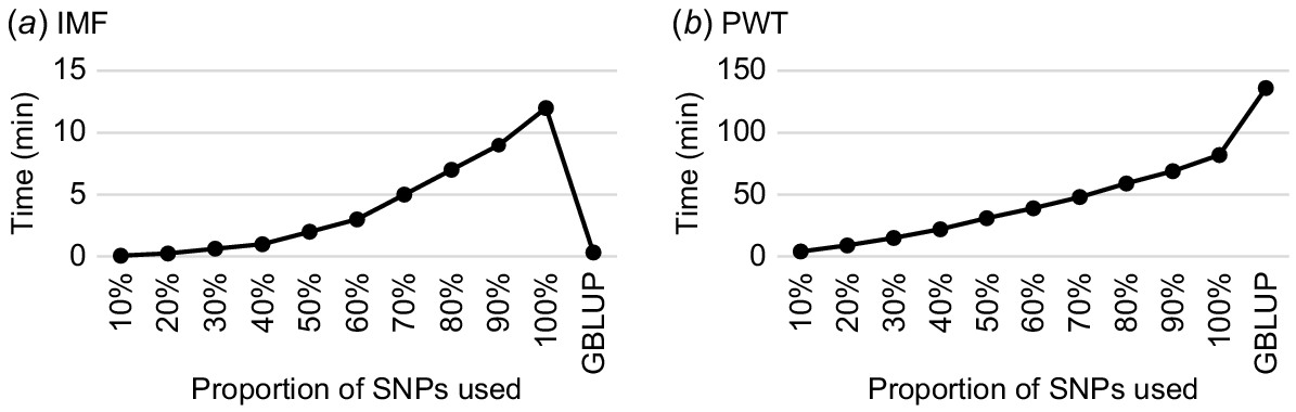
The PEVs obtained from the SNP–BLUP model by using all SNP markers for genotyped animals were found to be equivalent to those obtained from the GBLUP model for both IMF and PWT, as anticipated. When all 59 584 SNPs (100%) were used, computing time using the SNP–BLUP model was 43% less than that of the GBLUP model for PWT with 85 113 genotyped and phenotyped animals (Fig. 1). However, for IMF with 5784 genotyped and phenotyped animals, the GBLUP model was faster than SNP–BLUP for all SNPs (100%) and most subsets of SNPs (10–90% of total SNPs). Notably, for both IMF and PWT, the computing time decreased significantly as the number of SNPs in the subsets decreased in the SNP–BLUP model (Fig. 1). These results demonstrate that the SNP–BLUP model is more efficient when the number of genotyped and phenotyped animals exceeds the number of SNPs available.
Wall-clock time required to obtain PEVs in GBLUP and SNP–BLUP models, by using all SNPs (i.e. 100%) and nine subsets based on randomly selected 10%, 20%, …, and 90% of total SNPs (N = 59 584) for (a) intramuscular fat (IMF) and (b) post-weaning weight (PWT) from the MERINOSELECT sheep evaluation.
There were very high correlations (≥0.98) between PEVs calculated with all SNPs and most of the subsets of randomly selected SNPs for both IMF and PWT, except for the smallest (10%) subset for PWT (0.95) (Table 2). However, the mean PEV and the range decreased as the number of SNPs used in the subsets decreased. The same pattern was observed when the subsets of SNP were selected on the basis of the order of SNPs along the chromosomes (Table 3).
| IMF | PWT | |||||||||
|---|---|---|---|---|---|---|---|---|---|---|
| Proportion of SNPs used (%) | Mean | s.d. | Min | Max | Corr | Mean | s.d. | Min | Max | Corr |
| 100 | 0.422 | 0.044 | 0.117 | 0.659 | 1.00 | 0.184 | 0.034 | 0.040 | 0.476 | 1.00 |
| 90 | 0.421 | 0.043 | 0.116 | 0.656 | 1.00 | 0.181 | 0.033 | 0.038 | 0.467 | 1.00 |
| 80 | 0.419 | 0.043 | 0.115 | 0.656 | 1.00 | 0.177 | 0.032 | 0.036 | 0.454 | 1.00 |
| 70 | 0.417 | 0.043 | 0.114 | 0.651 | 1.00 | 0.172 | 0.031 | 0.035 | 0.445 | 1.00 |
| 60 | 0.415 | 0.043 | 0.114 | 0.645 | 1.00 | 0.165 | 0.030 | 0.032 | 0.422 | 1.00 |
| 50 | 0.410 | 0.042 | 0.113 | 0.636 | 1.00 | 0.157 | 0.028 | 0.030 | 0.398 | 1.00 |
| 40 | 0.405 | 0.042 | 0.110 | 0.632 | 1.00 | 0.146 | 0.026 | 0.025 | 0.377 | 1.00 |
| 30 | 0.398 | 0.041 | 0.101 | 0.622 | 0.99 | 0.130 | 0.022 | 0.021 | 0.319 | 0.99 |
| 20 | 0.382 | 0.039 | 0.094 | 0.587 | 0.99 | 0.106 | 0.017 | 0.015 | 0.257 | 0.98 |
| 10 | 0.342 | 0.035 | 0.074 | 0.549 | 0.98 | 0.063 | 0.009 | 0.008 | 0.133 | 0.95 |
Mean PEV (Mean), standard deviation (s.d.), minimum and maximum values (Min and Max), and correlations (Corr) with PEVs calculated with all SNPs (100%).
| IMF | PWT | |||||||||
|---|---|---|---|---|---|---|---|---|---|---|
| SNPs retained | Mean | s.d. | Min | Max | Corr | Mean | s.d. | Min | Max | Corr |
| All SNPs | 0.422 | 0.044 | 0.117 | 0.659 | 1.00 | 0.184 | 0.034 | 0.040 | 0.476 | 1.00 |
| 1 in 2 | 0.412 | 0.043 | 0.113 | 0.642 | 1.00 | 0.159 | 0.029 | 0.031 | 0.400 | 1.00 |
| 1 in 4 | 0.394 | 0.041 | 0.096 | 0.618 | 0.99 | 0.121 | 0.021 | 0.018 | 0.301 | 0.99 |
| 1 in 8 | 0.361 | 0.037 | 0.082 | 0.560 | 0.98 | 0.078 | 0.012 | 0.009 | 0.172 | 0.96 |
| 1 in 10 | 0.346 | 0.035 | 0.075 | 0.532 | 0.98 | 0.064 | 0.009 | 0.007 | 0.131 | 0.96 |
| 1 in 15 | 0.312 | 0.031 | 0.067 | 0.483 | 0.97 | 0.045 | 0.006 | 0.006 | 0.086 | 0.94 |
| 1 in 20 | 0.282 | 0.028 | 0.062 | 0.441 | 0.95 | 0.035 | 0.004 | 0.005 | 0.063 | 0.91 |
| 1 in 30 | 0.235 | 0.022 | 0.057 | 0.364 | 0.92 | 0.024 | 0.003 | 0.004 | 0.042 | 0.87 |
| 1 in 40 | 0.199 | 0.018 | 0.053 | 0.305 | 0.88 | 0.018 | 0.002 | 0.004 | 0.031 | 0.82 |
Mean PEV (Mean), standard deviation (s.d.), minimum and maximum values (Min and Max), and correlations (Corr) with PEVs calculated with all SNPs (100%).
The lowest correlation between PEVs from analysing a subset of SNPs compared with analysing the full set was for the smallest subset (every 40th SNP), namely 0.88 (IMF) and 0.82 (PWT). Mean, standard deviation and ranges were also lower as the amount of thinning increased. For the same number of SNPs, there was no significant difference between the PEVs by random selection and by thinning. For example, the mean PEV of random 10% SNPs and the correlation with all SNPs were 0.342 and 0.98 for IMF and 0.063 and 0.95 for PWT (Table 2), which were close to the PEVs observed when selecting every 10th SNP (1 in 10) (Table 3). A similar comparison can be made between a random selection of 50%, selecting every second SNP.
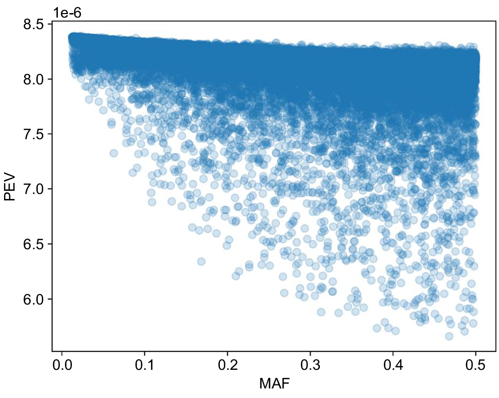
The PEVs for each SNP (i.e. the diagonals of C22 in Eqn 5 above) are shown by their allele frequency for IMF in Fig. 2. Unsurprisingly, SNPs with intermediate frequencies tend to have lower PEVs (higher accuracies) than do SNPs with extreme frequencies. Similar results were found for PWT (not shown).
Industry data sets
The computing times for PEV calculation based on the new SNP–BLUP method for the MERINOSELECT sheep and TACE beef evaluations are shown in Fig. 3. Across traits, computation times increased as the reference size increased, and decreased when the number of SNPs selected decreased. The equivalent GBLUP model could not be run on the server due to insufficient memory.
Computing times (wall-clock time, min) for each trait calculating PEV of genotyped animals using SNP–BLUP model for (a) the MERINOSELECT sheep evaluation from Feburary 2022 and (b) the Trans Tasman Angus Cattle Evaluation (TACE) from March 2022. Each trait is presented three times, once using all SNPs (59 583 for Merino and 70 026 for Angus), then every second SNP (2nd-SNP) and every fourth (4th-SNP) SNP.
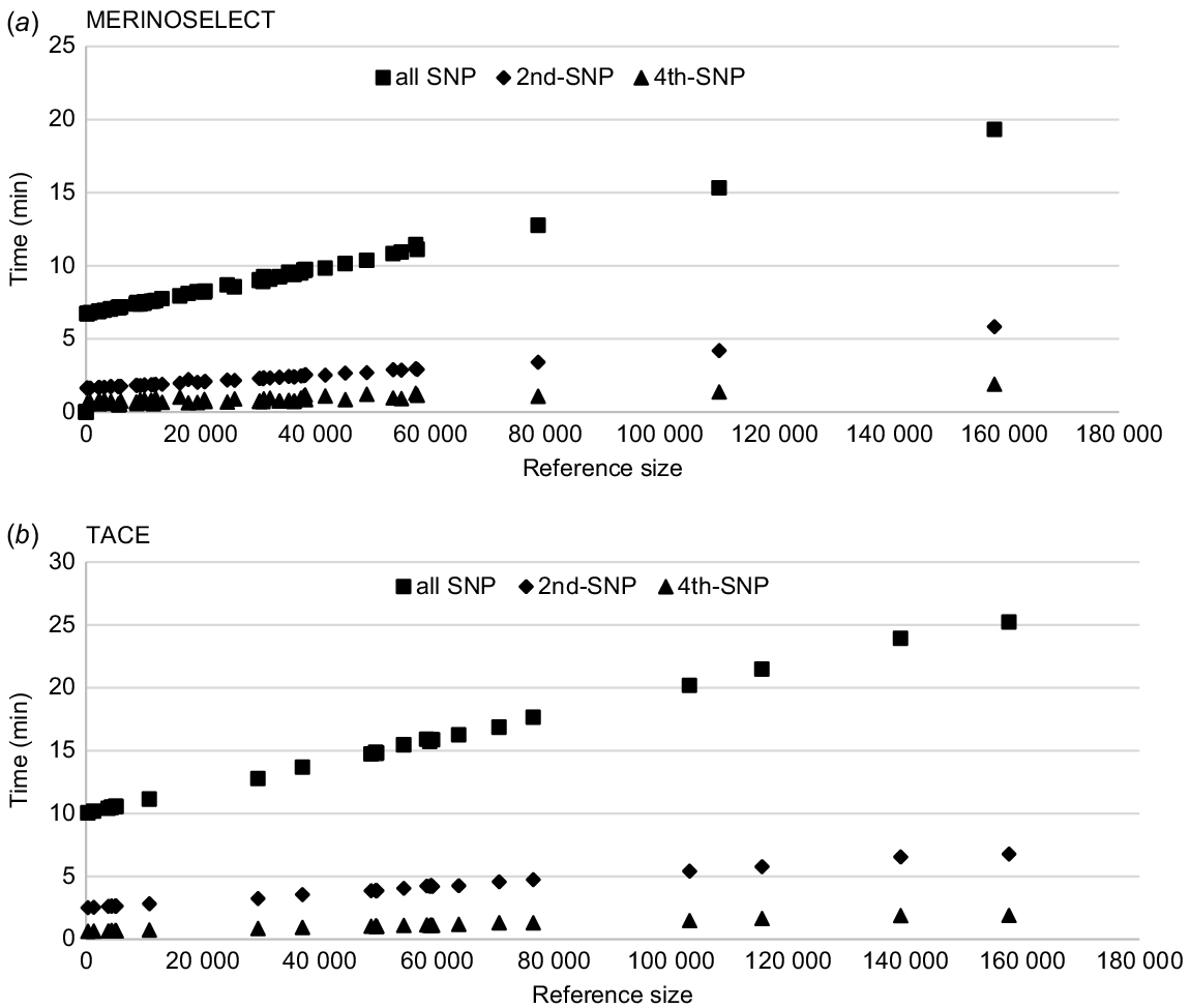
There were 61 traits (including eight maternal effects) in MERINOSELECT, and those with fewer than 60 000 reference animals took 6–12 min each. The maximum time was for a trait with about 160 000 reference animals. In the TACE data, of 28 traits (including four maternal effects), 24 traits had fewer than 80 000 reference animals, with computing time between 10 and 18 min each. As the total number of SNPs was 59 583 for MERINOSELECT and 70 026 for TACE, the computing time was longer for TACE, even given with similar reference population sizes. For example, computing times were about 20 min in MERINOSELECT and 25 min in TACE for the traits, with the largest references of ~160 000 animals in both (Fig. 3).
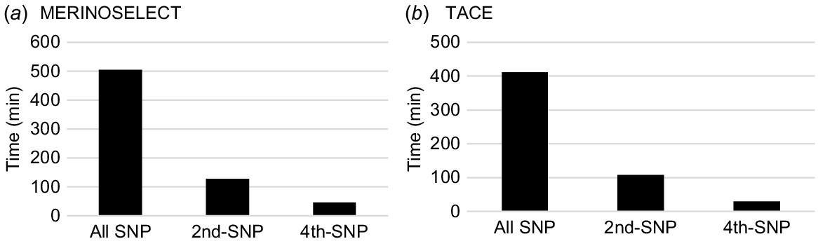
The total computing times across all traits were directly related to the total number of traits and the number of SNPs used in the SNP–BLUP model. They were ~500 min for all SNPs, ~129 min for the subset using every second SNP and ~47 min for the subset using every fourth SNP for MERINOSELECT. They were ~400 min for all SNPs, ~108 min for the subset using every second SNP, and ~29 min for the subset using every fourth SNP for TACE (Fig. 4).
Total computing times (wall-clock time, min) for calculating PEV of genotyped animals using SNP–BLUP model for 62 traits and eight maternal effects in a MERINOSELECT sheep evaluation from Feburary 2022 (a) and 24 traits and four maternal effects in a Trans Tasman Angus Cattle Evaluation (TACE) from March 2022 (b) using all SNPs, every second (2nd-SNP) and every fourth (4th-SNP) SNP.
Discussion
In Australia, the concept of EPNs from an animal’s own performance, its progeny, parents, correlated traits and genomic information has been successfully applied to approximate breeding-value accuracy in the BREEDPLAN beef cattle and Sheep Genetics single-step genetic evaluation systems. With the increasing numbers of genotyped animals, the derivation of genomic EPN based on the current GBLUP models was getting more and more difficult. This study focused on investigating an alternative method to calculating PEVs by a SNP–BLUP model to meet the most challenging part of the process. This study confirmed the equivalence of calculating PEVs via SNP–BLUP and GBLUP models and the efficiency of the SNP–BLUP when the number of genotyped and phenotyped animals is larger than the number of SNPs. The key calculation underpinning computation times for these methods is the inversion of the coefficient matrix, which benefits the SNP–BLUP approach when the number of genotyped and phenotyped animals exceeds the number of SNPs. Although most of the traits have fewer genotyped and phenotyped animals than SNPs used in the current genetic evaluation systems at this stage, performance benefits in terms of memory usage and computation times exist for highly recorded traits such as some weight traits. Traits with large numbers of reference animals are a major bottleneck in the PEV calculations in the current genetic evaluations.
For the implementation of this new SNP–BLUP model in the PEV approximation, a series of single-trait SNP–BLUP pseudo-analyses were conducted using Eqn 3 for genotyped animals. This model can fit fixed effects that were not included in the previous model (Li et al. 2017). This new improvement can account for an animal’s contemporary group as a fixed effect in the model. Furthermore, as X′X (in Eqn 5) is a diagonal matrix with the contemporary group size in the diagonal, the total group size including both genotyped and ungenotyped animals in a contemporary group is used instead of the group size for genotyped only animals. This model refinement is supposed to improve the approximation of PEVs.
When calculating for traits with large reference populations, there are usually two significant issues, namely, impractically long computing time and lack of computer memory. There are practical limits of ~200 000 genotyped animals for the GBLUP model for conducting the current Australian beef and sheep genetic evaluations with the existing computer capacity. The memory requirement is directly related to the size of the arrays required. In the implementation of this method, one optimisation performed was to use single precision for real variables with less precision required in accuracy approximations. This modification saves half of the memory usage for all those real vectors. For example, in the GBLUP model, a GRM of 180 000 genotypes stored at single precision requires 180 000 × 180 000 × 4 byte ≈ 121 Gb instead of 241 Gb for double precision. Memory usage for the SNP–BLUP model is reduced compared with the GBLUP model when the number of SNPs is smaller than the number of genotyped animals. For example, in the TACE data used here, the number of SNPs is about 70 000, and then the memory required to store the 70 000 by 70 000 SNP PEV matrix is ≈18 Gb with single precision.
Further, as SNP PEVs are converted to breeding-value PEVs, the memory usage requirements are reduced. As the number of predefined vectors and methods differ between the GBLUP and SNP–BLUP models, in general, the peak memory requirements for the SNP–BLUP model were found to be about one-third of the memory required for the GBLUP model for the data structures used in this study. To calculate Eqn 6, W has the dimensions of genotyped animals by SNPs. A dataset with 180 000 genotyped individuals and 70 000 SNPs would require 47 GB of memory. However, in most cases, we are not interested in the prediction-error covariance terms; the full W does not need to be stored in memory and can be calculated piece-wise for subsets of animals. This has not been implemented in the software described here, but allows for further memory savings as required in the future. Furthermore, the memory for the GBLUP model increases quadratically as the number of genotyped animals increases. However, if the number of markers remains constant, the memory needed for the SNP–BLUP model increases linearly with the increase of the genotyped animals. Therefore, the SNP–BLUP model is much more scalable with increasing numbers of animals genotyped.
If the number of markers increases, PEVs can still be calculated using subsets of SNPs by the SNP–BLUP model, with high correlations between PEVs from all SNPs and PEVs from subsets. Subsetting of SNPs was investigated by random selection and SNP thinning in this study, with a wide range of scenarios from 90% to 10% for random samplings and from every second to every 40th SNP for SNP thinning; both scenarios showed similar results when the number of SNPs was the same, indicating that the number of SNPs retained was more important than the method of subsetting. In this study, PEV based on the SNP–BLUP model using complete SNPs of ~60 000 was compared with PEVs using various subsets. The PEV using the total SNPs was highly correlated (1.0) with the PEV using randomly 50% or every second SNP (i.e. ~30 000), with a slight shrinkage distribution for the PEV using the subset. There were still very high correlations between PEV using complete SNPs and even 10% or every 10th SNP (i.e. the size of ~6000). However, the mean and standard deviation of PEVs decreases further as the size of the subset decreases, i.e. under-estimating of PEV occurs, which would lead to inflation of accuracies. These results were consistent with the findings of Sargolzaei et al. (2014) who also investigated the influence of subsets of SNPs on the approximation of reliability of EBVs. Therefore, caution should be taken to explore the proper subset size. This could be due to insufficient markers in linkage disequilibrium (LD) with the quantitative trait loci (QTL) affecting a specific trait in genomic selection. The number of markers needed to capture all genetic variance in genomic selection is related to the degree of LD decay in each species (Meuwissen and Goddard 2001); hence, defining subsets on the basis of LD pruning at different thresholds may be a more reasonable method to reduce the number of SNPs. The relationship between the marker PEV and the marker allele frequency showed that higher accuracy (lower PEV) of marker effects was found for those markers with intermediate frequency, suggesting that alternate sampling of SNPs on the basis of allele frequency and LD would be a good option.
One of the major advantages of genomic selection is to predict breeding values for genotyped animals that were not included in the genetic evaluations, i.e. young animals that have been genotyped since the latest analysis. Breeding values for these animals can be calculated as the sum of the SNP effects multiplied by its gene content. However, PEVs and, therefore, accuracies of those EBVs are non-trivial to calculate by the GBLUP model, although procedures have been proposed (Ferdosi et al. 2019). With the new SNP–BLUP model, the PEVs for these genotyped animals could be estimated by Eqn 5. With this flexibility, these animals could be compared with all other animals with the accuracy which is usually required by breeders to make selection decisions.
Conclusions
The SNP–BLUP model for PEV calculation for genotyped animals outperforms the GBLUP model regarding the compute cost. A new accuracy program (snpEPN) has been developed and used in routine sheep and beef genetic evaluation systems in Australia. This program provides an efficient and sustainable solution in PEV calculation to cater for increasing volumes of animals genotyped.
Data availability
Data used in this study were provided by MLA Sheep Genetics for MERINOSELECT data and Angus Australia for TACE data. Data were used on the condition that it will be kept confidential and cannot be shared publicly. Software developed as part of this research is commercial in confidence.
Acknowledgements
The authors acknowledge permission to access MERINOSELECT data from MLA Sheep Genetics, and TACE data from Angus Australia. We also acknowledge the contributions of dedicated breeders who contribute to these evaluation systems.
References
Ben Zaabza H, Mäntysaari EA, Strandén I (2020) Using Monte Carlo method to include polygenic effects in calculation of SNP-BLUP model reliability. Journal of Dairy Science 103, 5170-5182.
| Crossref | Google Scholar |
Ben Zaabza H, Van Tassell CP, Vandenplas J, VanRaden P, Liu Z, Eding H, McKay S, Haugaard K, Lidauer MH, Mäntysaari EA, Strandén I (2022) Invited review: reliability computation from the animal model era to the single-step genomic model era. Journal of Dairy Science 106, 1518-1532.
| Crossref | Google Scholar |
Bermann M, Lourenco D, Misztal I (2021) Efficient approximation of reliabilities for single-step genomic best linear unbiased predictor models with the algorithm for proven and young. Journal of Animal Science 100, skab353.
| Crossref | Google Scholar |
Brown DJ, Huisman AE, Swan AA, Graser H-U, Woolaston RR, Ball AJ, Atkins KD, Banks RB (2007) Genetic evaluation for the Australian sheep industry. Proceedings of the Association for the Advancement of Animal Breeding and Genetics 17, 187-194.
| Google Scholar |
Brown DJ, Swan AA, Boerner V, Li L, Gurman PM, McMillan AJ, van der Werf JHJ, Chandler HR, Tier B, Banks RG (2018) Single-step genetic evaluations in the Australian sheep industry. Proceedings of the World Congress on Genetics Applied to Livestock Production 11, 460.
| Google Scholar |
Edel C, Pimentel ECG, Erbe M, Emmerling R, Götz K-U (2019) Short communication: calculating analytical reliabilities for single-step predictions. Journal of Dairy Science 102, 3259-3265.
| Crossref | Google Scholar |
Ferdosi MH, Connors NK, Tier B (2019) An efficient method to calculate genomic prediction accuracy for new individuals. Frontiers in Genetics 10, 596.
| Crossref | Google Scholar |
Garcia A, Aguilar I, Legarra A, Tsuruta S, Misztal I, Lourenco D (2022) Theoretical accuracy for indirect predictions based on SNP effects from single-step GBLUP. Genetics Selection Evolution 54, 66.
| Crossref | Google Scholar |
Graser HU, Tier B (1997) Applying the concept of number of effective progeny to approximate accuracies of predictions derived from multiple trait analyses. Proceedings of the Association for the Advancement of Animal Breeding and Genetics 12, 547-551.
| Google Scholar |
Johnston DJ, Ferdosi MH, Connors NK, Boerner V, Cook J, Girard CJ, Swan AA, Tier B (2018) Implementation of single-step genomic BREEDPLAN evaluations in Australian beef cattle. Proceedings of the World Congress on Genetics Applied to Livestock Production 11, 269.
| Google Scholar |
Li L, Swan AA, Tier B (2017) Approximating the accuracy of single step EBVs. Proceedings of the Association for the Advancement of Animal Breeding and Genetics 22, 89-92.
| Google Scholar |
Liu Z, VanRaden PM, Lidauer M, Calus MPL, Benhajali H, Jorjani H, Ducrocq V (2017) Approximating genomic reliabilities for national genomic evaluation. Interbull Bulletin 51, 75-85.
| Google Scholar |
Meuwissen TH, Goddard ME (2001) Prediction of identity by descent probabilities from marker-haplotypes. Genetics Selection Evolution 33, 605–634.
| Crossref | Google Scholar |
Sargolzaei M, Schaeffer LR, Chesnais JP, Kistemaker G, Wiggans GR, Schenkel FS (2014) Approximation of reliability of direct genomic breeding values. Proceedings of the World Congress on Genetics Applied to Livestock Production 10, 485.
| Google Scholar |
Strandén I, Garrick DJ (2009) Technical note: derivation of equivalent computing algorithms for genomic predictions and reliabilities of animal merit. Journal of Dairy Science 92, 2971-2975.
| Crossref | Google Scholar |
VanRaden PM (2008) Efficient methods to compute genomic predictions. Journal of Dairy Science 91, 4414-4423.
| Crossref | Google Scholar |
Yang J, Benyamin B, McEvoy BP, Gordon S, Henders AK, Nyholt DR, Madden PA, Heath AC, Martin NG, Montgomery GW, Goddard ME, Visscher PM (2010) Common SNPs explain a large proportion of the heritability for human height. Nature Genetics 42, 565-569.
| Crossref | Google Scholar |