

Random regression models for multi-environment, multi-time data from crop breeding selection trials
J. De Faveri A B * , A. P. Verbyla A B and G. Rebetzke C
A CSIRO Data61, Atherton, Qld 4883, Australia.
B UQ QAAFI, St Lucia, Qld 4072, Australia.
C CSIRO Agriculture & Food Black Mountain, Canberra, ACT 2601, Australia.
Crop & Pasture Science 74(4) 271-283 https://doi.org/10.1071/CP21732
Submitted: 4 November 2021 Accepted: 13 July 2022 Published: 31 August 2022
© 2023 The Author(s) (or their employer(s)). Published by CSIRO Publishing. This is an open access article distributed under the Creative Commons Attribution-NonCommercial-NoDerivatives 4.0 International License (CC BY-NC-ND)
Abstract
Context: In order to identify best crop genotypes for recommendation to breeders, and ultimately for use in breeding, evaluation is usually conducted in field trials across a range of environments, known as multi-environment trials. Increasingly, many breeding traits are measured over time, for example with high-throughput phenotyping at different growth stages in annual crops or repeated harvests in perennial crops.
Aims: This study aims to provide an efficient, accurate approach for modelling genotype response over time and across environments, accounting for non-genetic sources of variation such as spatial and temporal correlation.
Methods: Because the aim is genotype selection, genetic effects are fitted as random effects, and so the approach is based on random regression, in which linear or non-linear models are used to model genotype responses. A method for fitting random regression is outlined in a multi-environment situation, using underlying cubic smoothing splines to model the mean trend over time. This approach is illustrated on six wheat experiments, using data on grain-filling over thermal time.
Key results: The method correlates genetic effects over time and environments, providing predicted genotype responses while incorporating spatial and temporal correlation between observations.
Conclusions: The approach provides robust genotype predictions by accounting for temporal and spatial effects simultaneously under various situations including those in which trials have different measurement times or where genotypes within trials are not measured at the same times. The approach facilitates investigation into genotype by environment interaction (G × E) both within and across environments.
Implications: The models presented have potential to increase accuracy of predictions over measurement times and trials, provide predictions at times other than those observed, and give a greater understanding of G × E interaction, hence improving genotype selection across environments for repeated-measures traits.
Keywords: crop variety selection, cubic smoothing splines, linear mixed models, MET, MEMT, multi-environment trials, random regression models, statistical genetics.
Introduction
The challenging objective of plant breeding programs is to improve crop performance through the development of new varieties. This requires the selection of the best performing breeding lines for traits of interest from breeding trials usually conducted across multiple environments (locations and years), known as multi-environment trials (METs). In order to optimise selection, it is important that the statistical methods used for analysing data from these breeding trials are as accurate and efficient as possible. A common approach for the analysis of METs is based on the linear mixed model (for a review, see Smith et al. 2005), which provides a flexible framework in which variety by trial effects can be modelled while accounting for within-trial error variation, for example due to spatial location, management practices and experimental design, even when data are unbalanced with not all varieties or breeding lines grown at all sites. Kelly et al. (2007) demonstrated the superiority of using linear mixed models with factor analytic (Smith et al. 2001) modelling of variety by trial effects, together with the spatial modelling approach of Gilmour et al. (1997), for selection of superior varieties in the MET situation.
Often, repeated measurements are taken on the plants within these breeding trials, for example multiple harvests in perennial crop trials, repeated sampling, or non-invasive measurements at various stages over the growth cycle of annual crops (e.g. with light detection and ranging (Rebetzke et al. 2016) or canopy temperature (Deery et al. 2016) through high-throughput phenotyping). The aim of these trials is to obtain accurate predictions for genotype performance over time and across a range of environments. Therefore, interest lies in the overall performance of varieties across time, as well as the interactions between genotype and time, genotype and environment, and genotype, time and environment.
Statistical analyses of data from such multi-environment, multi-time (MEMT) genotype selection trials need to model the genetic or genotype effects over time and sites in an appropriate way. These genotype effects may change over time and sites, and the effects may be correlated within and between sites. Because the aim of crop variety selection trials is selection of varieties, the standard approach is to treat these genotype effects as random effects. One approach to model the genotype effects over time is to model directly the variance–covariance matrix of genotype effects, for example using an unstructured genetic covariance model or factor analytic models. (Smith et al. 2007; De Faveri et al. 2015; Verbyla et al. 2021). This approach may be extended to the MET situation, using separable site by time models with unstructured or factor analytic models for each component, or by using a full direct modelling of the variance–covariance structure for sites by times using a factor analytic model (Smith et al. 2007; De Faveri 2013).
Although this approach may model the variance–covariance structure well, often the aim is to model the genetic response over time, and then to allow for prediction of genotype effects at times other than measurement times. The curves themselves may be of interest (De Faveri et al. 2015), and hence, a model for the (usually smooth) trend for genotypes over time is desired. An approach that allows for this is to model the genetic profiles over time using a random regression (or random coefficients) model (Laird and Ware 1982). The random regression model is commonly used to model lactation curves and cattle growth data (Meyer 1998, 2005a; Schaeffer 2004). It has also been applied in the genetic analysis of forestry trees at single sites (Apiolaza et al. 2000; Apiolaza and Garrick 2001; Wang et al. 2009), and single-site crop genetic analyses (De Faveri et al. 2015; Forknall et al. 2019), but its application in crop METs is limited. Often the random regression approach is implemented via orthogonal polynomials, Legendre or cubic polynomials (Campbell et al. 2018); however, more flexible bases such as splines can be used, for example B-splines (Meyer 2005b) or cubic smoothing splines (Verbyla et al. 1999; White et al. 1999; Huisman et al. 2002; DeGroot et al. 2003). Verbyla et al. (1999) used cubic smoothing spline random regression for modelling the unit effects in order to account for the temporal correlation between repeated observations, and De Faveri et al. (2015) used linear random regressions, with an underlying cubic smoothing spline for the mean response for persistence over time in a single lucerne breeding trial.
In the linear random regression models, the random intercepts and slopes are correlated to ensure that the model remains invariant to translation (Verbyla et al. 1999). When there are further spline random regression terms in the model, it is desirable to correlate all random intercept, slope and spline terms to ensure the model is invariant to a change in basis (White et al. 1999; Welham 2008; De Faveri 2013). However, fitting these models with a full set of correlations to ensure invariance to a change of basis is extremely difficult and often fails. Fortunately, in practice, although the underlying mean trend may require flexible spline modelling, the random variety or genotype deviations from the mean can often be modelled using simpler structures, for example linear or quadratic polynomial random regressions (Evans and Roberts 1979).
The genotype effects are the primary aim; however, they may be masked by non-genetic effects, which include effects due to the design of the trial and residual effects. It is important to model these non-genetic effects, including spatial and temporal correlation between observations within a trial (Smith et al. 2007; De Faveri et al. 2015; Verbyla et al. 2021).
In this paper, an approach will be presented for analysing data from MEMT crop genotype selection trials that accounts for both spatial and temporal variation and correlation within a trial, and also models the random genotype effects over time and trials, using underlying cubic smoothing splines, with linear deviations that are correlated across trials and times. The method of analysis was applied to data from a set of six experiments investigating repeated sampling of grainfill in wheat.
Materials and methods
Motivating data
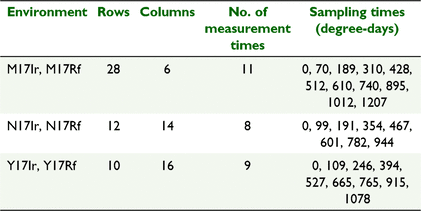
The motivating data come from a set of wheat genotype experiments conducted by CSIRO, investigating grain-filling over thermal days for 128 genotypes grown across six environments in 2017. The experiments were conducted at three locations (Narrabri, labelled N; Merredin, M; and Yanco, Y) with trials at each location being either irrigated (Ir) or rainfed (Rf), and hence grown as separate trials. The experiments were contained and managed in the national Managed Environment Facilities (Rebetzke et al. 2013). Each trial consisted of 128 entries in a partially replicated (p-rep) row–column design (Cullis et al. 2006) with 28 rows by 6 columns (168 plots) at M, 12 rows by 14 columns (168 plots) at N, and 10 rows by 16 columns at Y (160 plots).
The wheat genotypes represented high and low grain-filling wheats (Rebetzke et al. 2017) from four commercial breeding populations assessed in a previous study (G. Rebetzke, unpublished data). Several commercial and overseas introduced high grain-filling wheat varieties were also included. Plots were managed to control disease, and nutrients applied to maximise grain yield potential for the site. At each site, an irrigated treatment and a rainfed treatment were applied, with irrigation determined by measures of crop water use and soil-water availability (data not shown). Plots were monitored regularly for development and 15 ears harvested from each plot from immediately before flowering through to plot maturity. At each harvest, 15 heads were randomly sampled twice-weekly from each plot and then dried at 72°C for 4 days before weighing. Date of sampling was converted to thermal time (in degree-days) as the sum of daily mean temperature – base temperature (here assumed 0°C) from the first harvest (Day 0) to final harvest.
The trait investigated in this paper is ear weight over thermal time through grain-filling from immediately before flowering to harvest maturity. Data were collected on genotypes and control varieties in each experiment, over multiple times (8–11 measurement times, depending on the location) during the growing season, at varying degree-days, as given in Table 1. The aim of the trials to evaluate genotype responses for grainfill and investigate genotype by environment interaction for this trait.
|
A plot of the raw grainfill data over degree-days for the 128 genotypes in each environment is given in Fig. 1. The data show variation in ear dry weight over thermal time (in degree-days) between entries within a trial and differences between trials. The ear weight profiles follow a general similar overall trend with increasing weight over degree-days up to a point where the profiles flatten out and either reach an asymptote or start to decline. There are clear differences between environments, with N trials increasing more rapidly at the start than the other trials. Y trials increase more gradually and do not reach weights as high as the other trials. Note the difference in degree-day measurement times among the different locations (N, M and Y).

|
Statistical methods
De Faveri et al. (2015) presented a single-stage random regression analysis for repeated-measurement traits in crop variety selection trials for individual environments, based on a linear mixed model. A cubic smoothing spline was used to model the overall, non-linear mean underlying response profile, and a linear random regression was used to model the genotype deviations from the overall trend. In addition, the linear mixed model accounted for any residual spatial and temporal correlation present. Here, we extend the single-site approach to the multi-environment situation.
Suppose we have t trials in which m varieties are grown (not all varieties need to be grown in all trials). The jth trial consists of nj plots in a rectangular array consisting of cj columns by rj rows (nj = rjcj) and hj measurement times (degree-days in our study), which may vary across trials. The measurement times are given by tjk (k = 1,2,…,hj) for the jth trial. The total number of trial by time combinations is  , and the total number of observations is
  .
.
If yjs(i)(t) is the observation at time t for spatial location s (indexed by row and column) in trial j, with genotype i planted in that plot, the models fitted to the grain-filling data are of the form:

where all terms on the right-hand side are presented as dependent on time, although some need not be in some applications. The functions μj(t) represent an overall trend for each trial; fjs(t) are fixed effects (there could be several but they are represented by a single term here) that can depend on the trial and spatial location; uo,js(t) are non-genetic random effects that can depend on the trial and spatial location; and ejs(t) are residual effects, for example local spatial trends not explained by other terms in the model. The term ug,ij(t) is the genetic effect for genotype i at time t in trial j, and these effects are of primary interest.
Eqn 1 presents the observations as a continuous function of time, but the actual data are observed at the discrete sets of times given by tjk. Thus, let yj be the hjnj × 1 vector of observations for trial j, ordered as rows within columns within times. The data combined across trials are denoted by 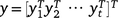 ; this is an N × 1 vector. Once all terms in Eqn 1 have been specified, a linear mixed model may be written for the data y (combined across times and trials) as:

where τ is a vector of fixed effects with design matrix X; ug is the h+m × 1 vector of genotype (or genetic) effects for individual trial by time combinations with associated design matrix Zg (N × h+m); uo is a vector of other random effects, with associated design matrix Zo; and e is the N × 1 vector of residuals.
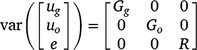
The random effects from the linear mixed model are assumed to follow a normal distribution with zero mean vector and variance–covariance matrix:
Modelling the underlying mean trend for each environment
The underlying mean trend for each environment (μj(t)) may be non-linear and may be modelled using polynomials. Alternatively, natural cubic smoothing splines (NCSS) (Verbyla et al. 1999) can be used to provide a more flexible specification. The NCSS (Green and Silverman 1994) can itself be formulated as a mixed model (Verbyla et al. 1999), with fixed terms (intercept and slope of a simple linear regression) for each environment. The curvature or non-linearity for each environment is included as an additional random effect with a variance parameter that relates to the underlying smoothing parameter of the NCSS. With the spline models, if there is replication it is possible to include a lack of fit or non-smooth random term, which is assumed to be independent and identically distributed. This term has been included for each environment in the analyses presented in this paper. All of the components described are trial-specific and contribute to Xτ and Zouo in Eqn 2.
Modelling non-genetic fixed and random effects
The only fixed effects in Eqn 2 are the fixed linear regressions for each trial; these are the fjs(t) of Eqn 1. Each trial was based on a row–column design, and hence for each trial by time combination, the block, row and column effects were included as non-genetic independent random effects, that is, in uo,js(t) in Eqn 1 and in Zouo in Eqn 2. In addition, a plot random effect at each trial connects the repeated measures over degree-days, also in uo,js(t) and Zouo.
Modelling residual effects
In METs, the full residual covariance matrix R is typically given by a block diagonal matrix:

where Rj is the residual variance matrix for the jth trial and diag forms a block diagonal matrix with blocks given by R1,R2,…,Rt. Therefore, each trial has its own residual covariance structure and residuals are assumed independent between trials.
The residual covariance matrix for the jth trial Rj models the spatial correlation and temporal correlation between repeated measurements in the trial. In this paper, these residual covariance matrices have been modelled using a three-way separable spatio-temporal process (Smith et al. 2007; De Faveri et al. 2015). Therefore, the structure is assumed to be:
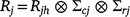
where Rjh is a covariance matrix that incorporates temporal correlation (between times) and possibly heterogeneous variance across times for trial j; and ∑cj and ∑rj are the column and row local spatial correlation matrices for trial j, here taken as autoregressive models of order 1 (ar1) with spatial correlation parameters ϕrj and ϕcj in the row and column directions, respectively (Gilmour et al. 1997). In the analyses, the temporal covariance components (Rjh) have been modelled using unstructured and ante-dependence models (Gabriel 1962; Kenward and Roger 1997). In these analyses, the separable residual models assume the same spatial correlation parameters ϕrj and ϕcj) for each time within each trial.
Modelling genetic effects
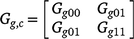
At the genetic level in MEMT trials, the aim is to model the interaction between trial, time within trial, and genotype. This is genotype by environment interaction (G × E), where environment not only includes location but also time effects. In general form, the variance matrix for these genetic effects across times and trials may be represented by  where Gth is a h+ × h+ genetic variance matrix indexed by all of the trial by time combinations, and Im is the assumed structure for the varieties (note that pedigree and/or genomic information could be included here, if available, to relate varieties via relationship matrices; see for example Oakey et al. 2006).
In the balanced (or near-balanced) case of the same number of times at the same times at each site, Smith et al. (2007) show that Gth may be modelled using a separable form, namely:

where Gt represents the trial genetic covariance structure (variances and covariances within and between trials), and Gh represents the time genetic covariance structure (variances and covariances for the times). The matrix Gt connects the environments and could be fully unstructured, or if t is large, a more parsimonious factor analytic structure (Smith et al. 2001, 2015) could be used, that is:

where Λt is a t × l matrix of loadings (l is the number of factors), and Ψt is a t × t diagonal matrix of the so-called specific variances. As the number of factors l increases, the approximation to a fully unstructured form generally improves. Note that the separable form (either unstructured or factor analytic) will require a constraint on the parameters for identifiability.
Note that, although the separable form Eqn 3 is desirable for ease of interpretation and computing advantages, the separable structure implies that the genetic correlation between pairs of times is the same for all trials. This may not be the case in practice.
The discussion above has focused on models for the variance structure of genetic effects. If the aim is to model the genotype responses over time using a continuous function, the random regression model (Laird and Ware 1982) provides a suitable approach for MEMT data.
Random regression approach
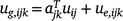
Although the underlying mean trend at each environment may be non-linear, the genotype deviations from this trend may often be linear over time (Evans and Roberts 1979), but they may vary over both varieties and environments. The intercept and slope of these lines may be taken as random rather than fixed, analogous to the basic quantitative genetics model in which genotype effects are taken as a random factor. If the genetic effects ug have components ug,ijk for genotype i, trial j and time k, where the actual time is tjk, a linear random regression model allowing for genotype by environment interactions is:

where uij0 and uij1 are the random intercept and slopes for genotype i at trial j; and ue,ijk is a residual deviation from the linear random regression, that is, a lack-of-fit term. The intercepts uij0 provide a prediction of performance at tjk = 0, so typically the time variable is centred so that the origin is at the midpoint, or average of the times. The slopes uij1 provide the rate of change of the effect of the genotype, and hence the speed at which the performance changes over time.
If  and
and  , Eqn 5 can be written as:
Putting the equations for varieties i together for site j and times tjk, we have:
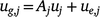
where the kth row of Aj is  ; and ug,j, uj and ue,j are vectors of total, linear random coefficients, and residual genotype effects for site j. For all sites, if A = diag(Aj), a block diagonal matrix with blocks Aj, the model for all genotype by time effects is:

In Eqn 6, both u and ue are independent random effects with zero mean. The linear random coefficients u have a variance matrix given by Gt2, where the t indicates dependence on the trials, and the two indicates linear (intercept and slope) for the time dimension; and the error or residual term ue has a variance matrix given by  .
.
The variance model for the genotype linear random regression effects u could be a separable or full structure. A separable structure for Gt2, the linear random coefficients across trials, would be of the form  , where:
is a (common across trials) 2 by 2 matrix of variances and covariances for intercepts and slopes. The matrix Gt can be unstructured or of factor analytic form given by Eqn 4.
As mentioned in the previous section, a separable structure may be too restrictive. A full structure for Gt2 is a 2t × 2t fully parameterised or unstructured variance matrix, which allows for differing variances and correlations of linear random coefficients both within and across trials. Again, if 2t is large, the fully unstructured covariance matrix may be difficult to fit, and then a more parsimonious factor analytic structure (Smith et al. 2001) may be used. In this case, like (Eqn 3):

where  is a 2t × l matrix of loadings, and Ψ is a 2t × 2t diagonal matrix.
Model comparison and testing
All analyses were performed in ASReml-R (Butler et al. 2018), using residual maximum likelihood (REML) estimation (Patterson and Thompson 1971) and best linear unbiased prediction (BLUP) of random effects (Robinson 1991). To test the significance of random effects in the linear mixed model, the residual maximum likelihood ratio test (REMLRT) can be used, but the distribution may be non-standard if the test involves variance parameters (see De Faveri et al. 2015). For non-nested models an information criterion, for example the Akaike information criterion (AIC), can be used, based on the full log-likelihood and REML estimates even if the fixed effects differ across models (Verbyla 2019).
Results
Analysis of each trial separately
First, an analysis of the data at each environment was conducted, in order to investigate spatial and temporal models for each trial. This analysis was based on a linear mixed model (as in Eqn 2 but for a single trial) (De Faveri et al. 2015). In each analysis, the mean underlying trend was modelled using a cubic smoothing spline, and linear random regressions were used to model the genotype deviations from the mean trend. Further genotype curvature was tested by fitting additional genotype cubic smoothing spline terms, but these were not statistically significant in all environments (although close to significant at N17Rf and Y17Rf; 0.05 < P < 0.10).
In each analysis, the random design terms for block, row and column for each measurement time were included in the model. In addition to accounting for the trial design, the spatial analysis approach of Gilmour et al. (1997) and Stefanova et al. (2009) was followed, including terms for extraneous and global trend and modelling local spatial correlation using a separable autoregressive process of order 1 in the row and column directions. Temporal correlation was incorporated into the model through three-way, separable spatio-temporal residual models together with a plot or unit/subject effect (Diggle 1988; De Faveri et al. 2015). Various spatio-temporal residual models were compared, using AIC, for each environment (Table 2).

|
The residual models tested for the single-site analyses included a single residual variance model (R1) with no account for spatial or temporal correlation and assuming a common variance across all times (Table 2). Although this model is not advocated, it is sometimes used, but as can be seen here (based on AIC comparisons), it is very restrictive and simplistic and can be greatly improved. The second residual model (R2) allowed for different residual variances for each time and separate ar1 spatial parameters in row and column directions at each time. There was no account for temporal correlation. The model was a significant (P < 0.05) improvement from R1 (Table 2). The third model (R3) was a separable residual model with different residual variances for each time (as in model R2) but included common spatial parameters across the times. Once again, this model did not incorporate temporal correlation between repeated measurements. This model was a significant (P < 0.05) improvement from model R2 at each environment (Table 2), indicating that in this case, a separable model assuming common spatial correlation parameters across the times could be suitable. The next model (R4) modelled the temporal correlation with an ante-dependence structure of order 1, using a three-way separable model. This model was a significant (P < 0.05) improvement on previous models, indicating the importance of modelling the temporal correlation. The final model (R5) also fitted a three-way separable spatio-temporal residual model, but this time used an unstructured covariance model for the temporal component. In this model, the plot term was omitted. This model was the best at five of the six environments (with M17Rf not converging) (Table 2). Hence, a mixture of ante-dependence and unstructured residual models (R4 for M17Rf and R5 for M17Ir, N17Ir, Y17Ir, N17Rf, Y17Rf) was chosen for the across-environment MET analysis, described in the following section.
Analysis of MET data (across trials)
The data were then combined across environments and a full MET random regression model (METRR) was fitted using Eqn 2. There was significant (P < 0.05) underlying curvature for the mean trend in each environment. In turn, this curvature was modelled using a separate cubic smoothing spline for each environment. The genotype deviations about the underlying environment mean responses were modelled using linear random regressions with correlated random intercepts and slopes, using a fully unstructured variance–covariance matrix of size 12 × 12. Thus, variances for all random intercepts and slopes for the six environments were estimated, as were the covariances (or correlations) for all pairs of the full set of 12 effects, and therefore 12 × 11/2 = 66 covariances or correlations.
The genetic variance components for the intercepts and slopes at each environment are presented in Table 3 (along the diagonal), and the genetic correlations between intercepts and slopes across and within environments are given off-diagonal.

|
As seen in Table 3, there was genetic variance for intercepts and slopes within each trial. There was genotype by environment variation, because the estimated genetic variances for intercepts differed across environments, as did the estimated variances for the slopes or linear trends; thus, the ‘average’ overall performance (intercepts) and the rate of change over time (slopes) exhibited G × E variation. Environments M17Ir, M17Rf, N17Ir and N17Rf had larger genetic variance for intercepts than Y17Ir and Y17Rf. These intercepts were predicted at the midpoint of degree-days across the trials (503 degree-days) and show that there was variation between genotypes in the actual level of ear weight at this point. The genetic variance for slopes was also greater for environments M17Ir, M17Rf, N17Ir and N17Rf than Y17Ir and Y17Rf. Large slope genetic variance indicates that varieties differed in their linear slope component of the non-linear response.
The genetic correlation between experiments for intercepts was high (0.78–0.99). Thus, the ranking of genotypes, in terms of their ‘average’ performance was similar across all environments. Similarly, the genetic correlation between experiments for slopes was high (0.61–0.99), and hence, the ranking of genotypes in terms of rate of change over time was similar across environments. The intercepts and slopes at each environment were highly correlated (0.92–0.99), and hence, genotypes that had high ear weight at the midpoint of degree-day measurements (503 degree-days) also had high slopes. Thus, genotypes with high ‘average’ performance also had high rate of change over time. Therefore, in terms of trends over time, there was little evidence for crossover of genotypes within a trial, and this is clear in Fig. 2 where the fitted curves for all genetic effects over time are presented.

|
In terms of the full set of genetic correlation between intercepts and slopes, the values were generally high (0.63–0.99), so that rankings of ‘average’ performance and rate of change were reasonably consistent, although not as high as within a trial.
A selection of genotypes and their predicted response profiles across thermal time for each environment is presented in Fig. 3. These genotypes were chosen from the full set of 128 entries because they exhibited high or low ear weight, or genotype by environment interaction. This can be seen more clearly in Fig. 4 where the linear deviations for each of these genotypes are plotted for each environment. For example, entries INQALAB91, SB169 and 3113 had consistently higher slope over all experiments, resulting in consistently higher ear weight and faster time to reach maximum weight. Some genotypes (e.g. SB171) had a very large slope in some experiments but smaller slope in others, showing G × E interaction. Some genotypes had consistent negative deviation slopes, indicating that they take longer to reach maximum and have smaller ear weight than average (e.g. DH_117, DH0085 and DH0117). Some genotypes had large negative slopes in some experiments but not at all (e.g. 3151 and 3133).

|

|
Plots of predicted intercepts (predicted at the midpoint 503 degree-days) against slopes for a subset of genotypes in the six experiments are shown in Fig. 5. In selection of better genotypes, those having both a large intercept and large slope may be preferred. For example, SB169 and INQALAB91 produce both large intercept and slope, whereas line 2995 is opposite, producing both a negative intercept and negative slope in all experiments (Fig. 5). Line 2995 could not be recommended based on performance and rate of filling. On the other hand, based on those criteria, line SB171 could be a recommended line in genotype selection. Thus, the pairs of intercepts and slopes provide a selection index in terms of grain-filling.

|
While genotype comparisons and interactions with environment may be investigated through the intercepts and slopes of genotype deviations from the underlying mean profiles, other measures can also be obtained for comparison. Of direct interest to the breeder is the maximum ear (grain) weight and time to reach maximum weight. By taking derivatives of the cubic smoothing splines for each genotype and equating to zero (Green and Silverman 1994; J De Faveri, AP Verbyla, G Rebetzke, in prep.), the time to maximum ear weight can be estimated and, hence, provide the maximum ear weight at this time. These measures are shown in Fig. 6.

|
Discussion
The analysis presented in this paper provides a single-stage approach for modelling repeated-measures traits in a multi-environment crop genotype or variety trial setting, correlating genetic effects over trials and times, while accounting for sources of non-genetic spatial and temporal correlation and trends. The approach allows insight into G × E by investigating the genetic variance matrix (Table 1). The approach also shows flexibility in providing robust solutions for situations where not all environments have the same number or range of measurement times.
In this analysis, linear random regressions were implemented for the genotype deviations from underlying environment mean profiles. The random intercepts and slopes were correlated across the six environments by using an unstructured 12 × 12 variance–covariance matrix. With further trials and, hence, more parameters to be correlated, the unstructured matrix may be difficult to fit; therefore, more parsimonious covariance models such as the factor analytic model could be used (Smith et al. 2001). ASReml-R (Butler et al. 2018) code for fitting both the unstructured and factor analytic models are given in Supplementary material File S1.
In this case, the variety deviations were able to be modelled using linear random regressions; however, other situations may require a non-linear model. For example, quadratic (or higher order polynomial) random regression terms could be used, in which case a full unstructured covariance matrix for the random coefficients would be required. Alternatively, a cubic smoothing spline could be used. In that case, a full set of covariances between the linear (intercepts and slopes) and the spline random effects would be required to provide a model that is invariant to translation and change of basis. In the cubic smoothing spline situation this can prove difficult in practice. Instead, it may be better to use B-splines, with coefficients correlated across trials. This is the subject of current research.
The approach presented here accounts for spatial and temporal correlation within a trial, using a three-way separable, spatio-temporal residual model, together with an overall plot or unit/subject effect. Although this separable model accounts for the important sources of variation, it is somewhat restrictive and assumes common spatial correlation parameters across the measurement times. In the example presented here, the separable model was shown to be a suitable option, but in other situations this assumption may not hold. More flexible residual models allowing for varying spatial correlation may provide an improvement, for example 2DIMVAR1 residual models (De Faveri et al. 2017) or three-dimensional tensor spline residual models (Verbyla et al. 2021). This is also the subject of further work.
The analysis enables prediction of genotype responses for grainfill and facilitates investigation into G × E interaction in the grainfill process among genotypes under different environments. The results show some entries with consistently higher ear weight and faster time to reach maximum ear weight across environments, and other entries with more variation in their response across environments. The splines implemented in this analysis provide a flexible approach to modelling the grainfill process with allowance for the non-asymptotic nature of the genotype responses. Resulting derivatives of the predicted splines allow for estimation of further traits of interest such as maximum weight, time to maximum, and a continuous rate of grainfill function (not presented here). This is in contrast to some classical two-stage methods of fitting curves such as the logistic or Gompertz to such data and subsequently analysing derived parameters. A comparison of these different approaches is the subject of a paper in preparation (J. De Faveri, A. P. Verbyla and G. Rebetzke).
The models presented in this paper result in accurate genetic predictions over measurement times and trials by optimally accounting for non-genetic effects, allowing for predictions at times other than those observed, and giving a greater understanding of G × E interaction, hence improving genotype selection across environments for repeated-measures traits.
Supplementary material
Supplementary material is available online.
Data availability
The data that support this study will be shared upon reasonable request to the corresponding author.
Conflicts of interest
The authors declare no conflicts of interest.
Declaration of funding
The authors thank the Grains Research and Development Corporation for funding both the experimental aspects of the Grain filling project and the statistical aspects through the SAGI-NORTH project.
References
Apiolaza LA, Garrick DJ (2001) Analysis of longitudinal data from progeny tests: some multivariate approaches. Forestry Science 47, 129–140.Apiolaza LA, Gilmour AR, Garrick DJ (2000) Variance modelling of longitudinal height data from a Pinus radiata progeny test. Canadian Journal of Forest Research 30, 645–654.
| Variance modelling of longitudinal height data from a Pinus radiata progeny test.Crossref | GoogleScholarGoogle Scholar |
Butler DG, Cullis BR, Gilmour AR, Gogel BJ, Thompson R (2018) ‘ASReml-R reference manual. Version 4.’ (VSN International: Hemel Hempstead, UK)
Campbell M, Walia H, Morota G (2018) Utilizing random regression models for genomic prediction of a longitudinal trait derived from high-throughput phenotyping. Plant Direct 2, 1–11.
| Utilizing random regression models for genomic prediction of a longitudinal trait derived from high-throughput phenotyping.Crossref | GoogleScholarGoogle Scholar |
Cullis BR, Smith AB, Coombes NE (2006) On the design of early generation variety trials with correlated data. Journal of Agricultural, Biological, and Environmental Statistics 11, 381–393.
| On the design of early generation variety trials with correlated data.Crossref | GoogleScholarGoogle Scholar |
De Faveri J (2013) Spatial and temporal modelling of perennial crop variety selection trials. PhD Thesis, The University of Adelaide, SA, Australia. Available at http://digital.library.adelaide.edu.au/dspace/handle/2440/83114
De Faveri JD, Verbyla AP, Pitchford WS, Venkatanagappa S, Cullis BR (2015) Statistical methods for analysis of multi-harvest data from perennial pasture variety selection trials. Crop & Pasture Science 66, 947–962.
| Statistical methods for analysis of multi-harvest data from perennial pasture variety selection trials.Crossref | GoogleScholarGoogle Scholar |
De Faveri J, Verbyla AP, Cullis BR, Pitchford WS, Thompson R (2017) Residual variance–covariance modelling in analysis of multivariate data from variety selection trials. Journal of Agricultural, Biological and Environmental Statistics 22, 1–22.
| Residual variance–covariance modelling in analysis of multivariate data from variety selection trials.Crossref | GoogleScholarGoogle Scholar |
Deery DM, Rebetzke GJ, Jimenez-Berni JA, James RA, Condon AG, Bovill WD, Hutchinson P, Scarrow J, Davy R, Furbank RT (2016) Methodology for high-throughput field phenotyping of canopy temperature using airborne thermography. Frontiers in Plant Science 7, 1808
| Methodology for high-throughput field phenotyping of canopy temperature using airborne thermography.Crossref | GoogleScholarGoogle Scholar |
DeGroot BJ, Keown JF, Kachman SD, Van Vleck D (2003) Cubic splines for estimating lactation curves and genetic parameters of first lactation Holstein cows treated with bovine somatotropin. Conference on Applied Statistics in Agriculture 1, 150–163.
| Cubic splines for estimating lactation curves and genetic parameters of first lactation Holstein cows treated with bovine somatotropin.Crossref | GoogleScholarGoogle Scholar |
Diggle P (1988) An approach to the analysis of repeated measurements. Biometrics 44, 959–971.
Evans JC, Roberts EA (1979) Analysis of sequential observations with applications to experiments on grazing animals and perennial plants. Biometrics 35, 687–693.
| Analysis of sequential observations with applications to experiments on grazing animals and perennial plants.Crossref | GoogleScholarGoogle Scholar |
Forknall CR, Simpfendorfer S, Kelly AM (2019) Using yield response curves to measure variation in the tolerance and resistance of wheat cultivars to fusarium crown rot. Phytopathology 109, 932–941.
| Using yield response curves to measure variation in the tolerance and resistance of wheat cultivars to fusarium crown rot.Crossref | GoogleScholarGoogle Scholar |
Gabriel KR (1962) Ante-dependence analysis of an ordered set of variables. The Annals of Mathematical Statistics 33, 201–212.
| Ante-dependence analysis of an ordered set of variables.Crossref | GoogleScholarGoogle Scholar |
Gilmour AR, Cullis BR, Verbyla AP (1997) Accounting for natural and extraneous variation in the analysis of field experiments. Journal of Agricultural, Biological, and Environmental Statistics 2, 269–293.
| Accounting for natural and extraneous variation in the analysis of field experiments.Crossref | GoogleScholarGoogle Scholar |
Green PJ, Silverman BW (1994) ‘Nonparametric regression and generalised linear models.’ (Chapman and Hall: London, UK)
Huisman AE, Veerkamp RF, van Arendonk JAM (2002) Genetic parameters for various random regression models to describe the weight data of pigs. Journal of Animal Science 80, 575–582.
| Genetic parameters for various random regression models to describe the weight data of pigs.Crossref | GoogleScholarGoogle Scholar |
Kelly AM, Smith AB, Eccleston JA, Cullis BR (2007) The accuracy of varietal selection using factor analytic models for multi-environment plant breeding trials. Crop Science 47, 1063–1070.
| The accuracy of varietal selection using factor analytic models for multi-environment plant breeding trials.Crossref | GoogleScholarGoogle Scholar |
Kenward M, Roger J (1997) The precision of fixed effects estimates from restricted maximum likelihood. Biometrics 53, 983–997.
Laird NM, Ware JH (1982) Random-effects models for longitudinal data. Biometrics 38, 963–974.
| Random-effects models for longitudinal data.Crossref | GoogleScholarGoogle Scholar |
Meyer K (1998) Estimating covariance functions for longitudinal data using a random regression model. Genetics Selection Evolution 30, 221
| Estimating covariance functions for longitudinal data using a random regression model.Crossref | GoogleScholarGoogle Scholar |
Meyer K (2005a) Random regression analyses using B-splines to model growth of Australian Angus cattle. Genetics Selection Evolution 37, 473
| Random regression analyses using B-splines to model growth of Australian Angus cattle.Crossref | GoogleScholarGoogle Scholar |
Meyer K (2005b) Advances in methodology for random regression analyses. Australian Journal of Experimental Agriculture 45, 847–858.
| Advances in methodology for random regression analyses.Crossref | GoogleScholarGoogle Scholar |
Oakey H, Verbyla A, Pitchford W, Cullis B, Kuchel H (2006) Joint modeling of additive and non-additive genetic line effects in single field trials. Theoretical and Applied Genetics 113, 809–819.
| Joint modeling of additive and non-additive genetic line effects in single field trials.Crossref | GoogleScholarGoogle Scholar |
Patterson HD, Thompson R (1971) Recovery of interblock information when block sizes are unequal. Biometrika 31, 100–109.
Rebetzke GJ, Chenu K, Biddulph B, Moeller C, Deery DM, Rattey AR, Bennett D, Barrett-Lennard EG, Mayer JE (2013) A multisite managed environment facility for targeted trait and germplasm phenotyping. Functional Plant Biology 40, 1–13.
| A multisite managed environment facility for targeted trait and germplasm phenotyping.Crossref | GoogleScholarGoogle Scholar |
Rebetzke GJ, Jimenez-Berni JA, Bovill WD, Deery DM, James RA (2016) High-throughput phenotyping technologies allow accurate selection of stay-green. Journal of Experimental Botany 67, 4919–4924.
| High-throughput phenotyping technologies allow accurate selection of stay-green.Crossref | GoogleScholarGoogle Scholar |
Rebetzke GJ, Richards RA, Holland JB (2017) Population extremes for assessing trait value and correlated response of genetically complex traits. Field Crops Research 201, 122–132.
| Population extremes for assessing trait value and correlated response of genetically complex traits.Crossref | GoogleScholarGoogle Scholar |
Robinson GK (1991) That BLUP is a good thing: the estimation of random effects. Statistical Science 6, 15–51.
Schaeffer LR (2004) Application of random regression models in animal breeding. Livestock Production Science 86, 35–45.
| Application of random regression models in animal breeding.Crossref | GoogleScholarGoogle Scholar |
Smith A, Cullis B, Thompson R (2001) Analysing variety by environment data using multiplicative mixed models and adjustments for spatial field trend. Biometrics 57, 1138–1147.
| Analysing variety by environment data using multiplicative mixed models and adjustments for spatial field trend.Crossref | GoogleScholarGoogle Scholar |
Smith AB, Cullis BR, Thompson R (2005) The analysis of crop cultivar breeding and evaluation trials: an overview of current mixed model approaches. The Journal of Agricultural Science 143, 449–462.
| The analysis of crop cultivar breeding and evaluation trials: an overview of current mixed model approaches.Crossref | GoogleScholarGoogle Scholar |
Smith AB, Stringer JK, Wei X, Cullis BR (2007) Varietal selection for perennial crops where data relate to multiple harvests from a series of field trials. Euphytica 157, 253–266.
| Varietal selection for perennial crops where data relate to multiple harvests from a series of field trials.Crossref | GoogleScholarGoogle Scholar |
Smith AB, Ganesalingam A, Kuchel H, Cullis BR (2015) Factor analytic mixed models for the provision of grower information from national crop variety testing programs. Theoretical and Applied Genetics 128, 55–72.
| Factor analytic mixed models for the provision of grower information from national crop variety testing programs.Crossref | GoogleScholarGoogle Scholar |
Stefanova KT, Smith AB, Cullis BR (2009) Enhanced diagnostics for the spatial analysis of field trials. Journal of Agricultural, Biological, and Environmental Statistics 14, 392
| Enhanced diagnostics for the spatial analysis of field trials.Crossref | GoogleScholarGoogle Scholar |
Verbyla AP (2019) A note on model selection using information criteria for general linear models estimated using REML. Australian & New Zealand Journal of Statistics 61, 39–50.
| A note on model selection using information criteria for general linear models estimated using REML.Crossref | GoogleScholarGoogle Scholar |
Verbyla AP, Cullis BR, Kenward MG, Welham SJ (1999) The analysis of designed experiments and longitudinal data by using smoothing splines. Journal of the Royal Statistical Society: Series C (Applied Statistics) 48, 269–311.
| The analysis of designed experiments and longitudinal data by using smoothing splines.Crossref | GoogleScholarGoogle Scholar |
Verbyla AP, De Faveri J, Deery DM, Rebetzke GJ (2021) Modelling temporal genetic and spatio-temporal residual effects for high-throughput phenotyping data. Australian & New Zealand Journal of Statistics 63, 284–308.
| Modelling temporal genetic and spatio-temporal residual effects for high-throughput phenotyping data.Crossref | GoogleScholarGoogle Scholar |
Wang C, Andersson B, Waldmann P (2009) Genetic analysis of longitudinal height data using random regression. Canadian Journal of Forest Research 39, 1939–1948.
| Genetic analysis of longitudinal height data using random regression.Crossref | GoogleScholarGoogle Scholar |
Welham SJ (2008) Smoothing spline models for longitudinal data. In ‘Longitudinal data analysis’. (Eds G Fitzmaurice, M Davidian, G Verbeke, G Molenberghs) pp. 253–289. (Chapman and Hall: London, UK)
White IMS, Thompson R, Brotherstone S (1999) Genetic and environmental smoothing of lactation curves with cubic splines. Journal of Dairy Science 82, 632–638.
| Genetic and environmental smoothing of lactation curves with cubic splines.Crossref | GoogleScholarGoogle Scholar |