

Proximal and remote sensing – what makes the best farm digital soil maps?
Patrick Filippi A * , Brett M. Whelan A and Thomas F. A. Bishop A
A
Abstract
Digital soil maps (DSM) across large areas have an inability to capture soil variation at within-fields despite being at fine spatial resolutions. In addition, creating field-extent soil maps is relatively rare, largely due to cost.
To overcome these limitations by creating soil maps across multiple fields/farms and assessing the value of different remote sensing (RS) and on-the-go proximal (PS) datasets to do this.
The value of different RS and on-the-go PS data was tested individually, and in combination for mapping three different topsoil and subsoil properties (organic carbon, clay, and pH) for three cropping farms across Australia using DSM techniques.
Using both PS and RS data layers created the best predictions. Using RS data only generally led to better predictions than PS data only, likely because soil variation is driven by a number of factors, and there is a larger suite of RS variables that represent these. Despite this, PS gamma radiometrics potassium was the most widely used variable in the PS and RS scenario. The RS variables based on satellite imagery (NDVI and bare earth) were important predictors for many models, demonstrating that imagery of crops and bare soil represent variation in soil well.
The results demonstrate the value of combining both PS and RS data layers together to map agronomically important topsoil and subsoil properties at fine spatial resolutions across diverse cropping farms.
Growers that invest in implementing this could then use these products to inform important decisions regarding management of soil and crops.
Keywords: broadacre cropping, digital soil mapping, precision agriculture, proximal sensing, remote sensing, soil constraints, soil spatial variability.
Introduction
Digital soil mapping (DSM) has been gaining in popularity over the past few decades, and this has been driven by the abundance of spatial datasets and increased computing power and data analytical techniques now available. There have been a large number of reviews written on DSM in recent years (e.g. McBratney et al. 2019; Searle et al. 2021), but it is an area of research that still has many challenges to overcome for the products to provide genuine value to a range of stakeholders. The majority of DSM studies are conducted across large areas, with many researchers often trying to map as large an area as possible (Grunwald et al. 2011; Arrouays et al. 2017). While these studies often predict at fine spatial resolutions (e.g. 30 m) over large extents, a problem is that the maps do not represent fine-scale variability well, such as the variation within an agricultural field. While many DSM studies promote the importance of the products for farmers, many farmers do not know they exist; or if they do, they may not trust the quality of the predictions. A study by Han et al. (2022) demonstrated how poor global, national, and state DSM products were at representing within-farm variability across a collection of diverse cropping fields and farms in Australia.
Creating bespoke DSM products for farmers at the field extent is less common, primarily due to the large expense of collecting samples (this varies by region/country), and the lack of skilled practitioners. Mapping soil within-fields is usually a step towards implementing management practices using precision agriculture principles. One common approach is to implement a grid sampling approach and use a simple interpolation technique such as inverse distance weighting (IDW) to create spatial maps.
However, to capture the true scale of variation in soil across space data often needs to be collected on dense grids, which can be a prohibitively expensive task (Kerry et al. 2010). Another common approach is to collect proximally-sensed data (e.g. from an electromagnetic induction sensor) and then strategically sample soil based on this information. This can be a more cost-effective approach as fewer soil samples are often required to cover the extent of variability compared to standard grid sampling (Kerry et al. 2010). When this latter approach is adopted, operators generally use simple approaches, such as using a single spatial variable to create models and maps. Nonetheless, cost can still be a limitation in these scenarios. A typical farmer in Australia can often have more than 10 fields, and having enough soil observations per field to create a simple linear model is generally a challenge. Many commercial operators in Australia work off a sampling density of one sample per 50–100 ha as this is something that can be realistically implemented (SPAA 2022).
In Australia, over half of the continent is used for agriculture. So creating useful and affordable soil maps is an important step to help farmers in improving the management of our soils. Given the issues raised above, a promising approach is to create bespoke soil maps for whole farms, as opposed to individual fields. While traditional precision agriculture focused on single fields in isolation, there has recently been a shift to combining data from multiple fields for analysis (Filippi et al. 2019a). This is due to a few reasons, such as the high cost of sampling and analysing soil, and the fact that more data can be utilised as it is from multiple fields. However this presents some challenges, for example, differences in management practices between fields (e.g. crop rotations) can result in differences in the state of soil properties (e.g. moisture), which can then impact on the data collected by proximal sensors. This has the potential to impact the value and usefulness of proximal sensing when modelling and mapping across multiple fields.
Proximal sensing is described as using a sensor in contact, or within 2 m of the soil, whereas remote sensing is described as using a sensor at least 2 m from the soil (Tilse et al. 2023). There are different components of proximal sensing, but for the purpose of this paper, we refer to sensors that are best described as on-the-go proximal sensors. This includes sensors such as electromagnetic induction (EM), or gamma radiometric sensors which are typically mounted to a ground-based vehicle and measurements are taken and recorded as the vehicle passes over fields. This is opposed to handheld, point-based proximal sensors such as visible near-infrared sensors. A more detailed description of these different types of technologies can be found in Tilse et al. (2023).
Using on-the-go proximal sensing data has been seen as the gold standard for DSM at the smaller scale. However, there is now an abundance of data collected by various remote sensors that can represent the within-field variability of soil. For example, in Australia there is now public access to airborne gamma radiometrics data (Minty et al. 2009), elevation and terrain attributes (CSIRO 2023), bare earth (BE) imagery (Roberts et al. 2019), and imagery from a range of satellites such as Landsat and Sentinel (Gorelick et al. 2017). While combining proximal data with remotely-sensed data is not a new concept, there is often a view by the industry (e.g. commercial service providers) that if proximal sensing data is present, there is limited value in the addition of remote sensing data. However, variation in soil properties is driven by a number of different factors and their interactions, and these proximal and remote sensing variables can provide surrogates that represent these.
This study aims to assess the value of different proximal and remote sensing data individually, as well as the combination of the two for mapping three different important soil properties (organic carbon, clay, and pH). This is done across multiple fields for three farms in different biogeographical locations across Australia, and in the topsoil (0–10 cm) and subsoil (30–60 cm). This could guide decisions about whether or not growers should invest in collecting proximally-sensed data. This study aims to demonstrate a robust, realistic, and cost-effective approach to mapping soil properties at the whole-farm scale for farmers and land managers which could be valuable in informing management decisions.
Materials and methods
Study sites and soil datasets
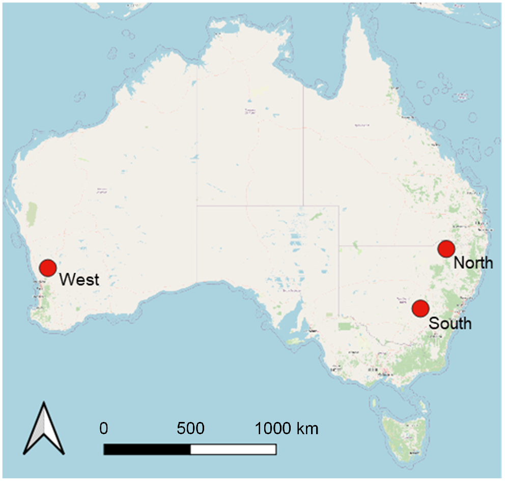
Three different farm sites were used in this study: (1) a farm in the wheatbelt of Western Australia, ‘West Farm’ (7200 ha); (2) a farm in northern NSW, ‘North Farm’ (4900 ha); and (3) a farm in southern NSW, ‘South Farm’ (2000 ha) (Fig. 1). West Farm has a mix of soil types, typically of sandier texture and gravel layers; North Farm is characterised by uniformly textured clay soils; and South Farm has a mix of duplex and gradational textured soil types. Soil cores were extracted and sub-sampled at 0–10 cm and 30–60 cm depths.
Soil pH (1:5 soil:H20) was measured by a pH meter with an ion-selective electrode. Organic carbon was measured by the combustion method as no carbonates were present in any samples. Soil carbon data was only available for the topsoil. Soil clay content was assessed by the hydrometer method. These particular soil properties were chosen as they contribute to important characteristics of soil, such as water holding capacity, chemical constraints, and nutrient availability, and are of key interest to farmers.
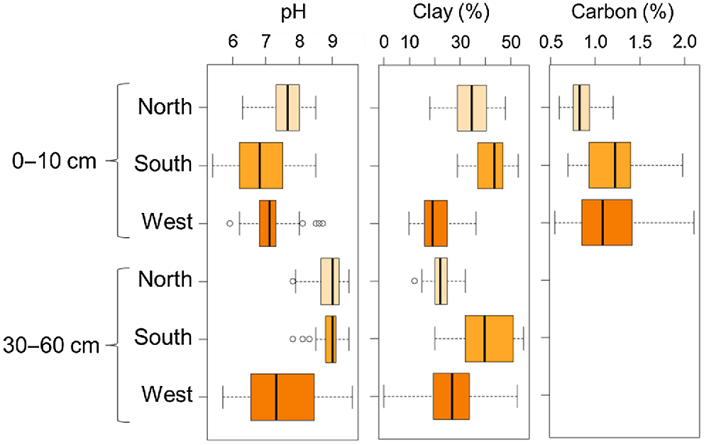
In terms of median pH values, North Farm had the highest topsoil pH, as well as alkaline subsoils (Fig. 2). South Farm was characterised by a more acidic topsoil and an alkaline subsoil. West Farm had consistent neutral median pH values, but with quite a bit of variation in the subsoil. Clay content was highest overall for South Farm, followed by North Farm and then West Farm. South Farm had the highest median topsoil organic carbon content, which was then followed by West Farm and then North Farm.
Summary statistics of the soil laboratory analysis for pH, clay content, and organic carbon content across the three study farms and two sampled depths.
The number of sampling sites where a soil core was extracted for each farm varied from 22 to 91, relative to the size of the farm (Table 1). In Australia, soil sampling and analysis is expensive, and realistically growers and land managers are restricted by the cost. Although a larger number of samples would likely produce more accurate predictions, the reality is that this is not economically feasible. The sampling density for this study ranges from one sample per ~80–100 ha.
| Farm | Farm size (ha) | No. of sites | Number of fields | Proximal electromagnetic induction available | Proximal gamma available | |
|---|---|---|---|---|---|---|
| West Farm | 7200 | 91 | 52 | 50 cm, 150 cm | K, Th, U, TC | |
| North Farm | 4900 | 48 | 5 | 50 cm, 150 cm | K | |
| South Farm | 2000 | 22 | 4 | 50 cm, 150 cm | K |
K, potassium; Th, thorium; U, uranium; TC, total count.
Proximally-sensed data
A proximal soil sensing survey was conducted to collect high-resolution apparent soil electrical conductivity (ECa) and gamma radiometrics data. The proximal soil sensing survey was conducted on 24 m swaths, and the position was recorded with differential GPS (DGPS) equipment. Continuous surface layers were obtained by kriging with local variograms onto a standard 10-m grid through the software R (R Core Team 2020).
Apparent soil electrical conductivity (ECa) was measured via EM using a DUALEM-21S instrument (Dualem Inc., Milton, Ontario, Canada). Information representing depths to 50 cm and 150 cm of the profile was used for all farms in this study (Fig. 3).
Gamma radiometric data was recorded using an RSX-1 gamma radiometric detector with a 4 L Sodium-Iodine crystal (Radiation Solutions Inc., Mississauga, Ontario, Canada). Data for potassium (K), thorium (Th), uranium (U), and total dose were available for West Farm, however, only K was available for both North Farm and South farm.
Remotely-sensed data
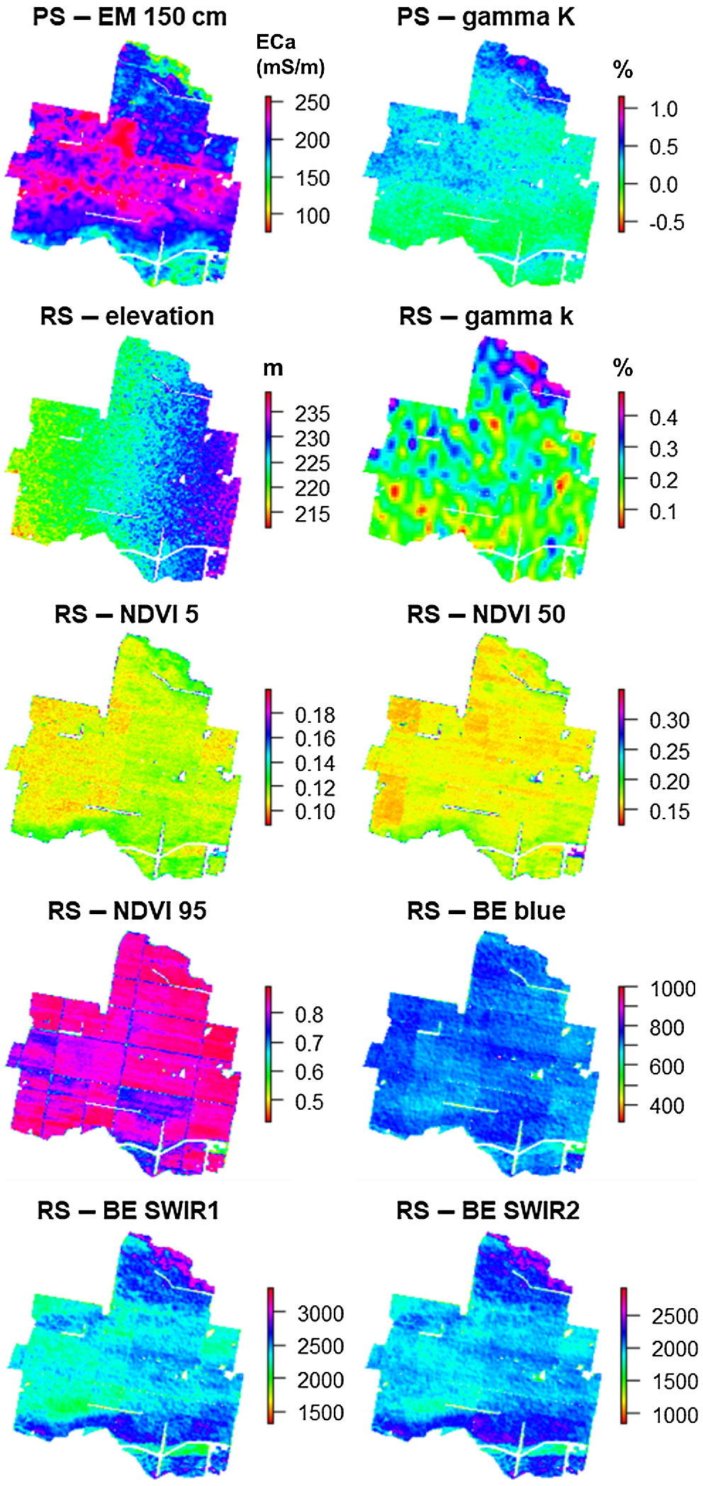
A subset of covariate maps are in Fig. 3 for North Farm as an example. This subset was chosen to showcase the differences in spatial variation and patterns for each different type of data described in Table 2.
| Data type | Category | Data description | Spatial resolution (m) | |
|---|---|---|---|---|
| Proximallysensed data | Electro-magnetic induction | ECa 50 cm | 10 | |
| ECa 150 cm | 10 | |||
| Ground-based gamma radiometrics | Potassium (%) | 10 | ||
| Thorium (ppm) | 10 | |||
| Uranium (ppm) | 10 | |||
| Total dose | 10 | |||
| Remotely-sensed data | Terrain attributes | DEM (m) | 30 | |
| TWI | 30 | |||
| Airborne gamma radiometrics | Potassium (%) | 100 | ||
| Thorium (ppm) | 100 | |||
| Uranium (ppm) | 100 | |||
| Total dose | 100 | |||
| Landsat NDVI | NDVI 5th percentile [2000–2020] | 30 | ||
| NDVI 50th percentile [2000–2020] | 30 | |||
| NDVI 95th percentile [2000–2020] | 30 | |||
| Landsat bare earth image | Blue band | 25 | ||
| Red band | 25 | |||
| Green band | 25 | |||
| NIR band | 25 | |||
| SWIR1 band | 25 | |||
| SWIR2 band | 25 |
ECa, soil electrical conductivity; DEM, digital elevation model; TWI, topographic wetness index; NIR, near infra-red; SWIR, shortwave infra-red; NDVI, normalised difference vegetation index.
A digital elevation model (DEM) at ~30 m resolution derived from the Shuttle Radar Topography Mission (SRTM) acquired by NASA (Farr et al. 2007) was obtained from the ELVIS (ELeVation Information System) platform (Department of Finance, Services, and Innovation 2023). A map of topographic wetness index (TWI), which was also derived from the SRTM, was downloaded through CSIRO’s Data Access Portal (CSIRO 2023).
Air-borne gamma radiometric potassium, thorium, uranium, and total dose data was obtained through the Geophysical Archive Data Delivery System (GADDS), Geoscience Australia. This data is known to represent the parent material of the soil, and soil types. This data was collected on varying swath widths across Australia and is provided as a ~100-m resolution gridded product. Airborne radiometric products were processed with a low pass filter to remove noise (Minty et al. 2009).
NDVI imagery from the Landsat 7 satellite at a ~30-m resolution was obtained from 1 January 2000 to 31 December 2020. A cloud-masking filter was applied to these images to remove all pixels that were affected by cloud cover. The 5th, 50th and 95th percentile statistics were then calculated to represent the most common value (50th percentile, or median), and the lower and upper distribution of the imagery (5th and 95th percentile, respectively) over the time period. These different percentiles of NDVI reflect long-term trends in crop biomass, and therefore a surrogate for variation in production.
BE imagery for the Australian continent is available from https://nationalmap.gov.au/, and is described by Roberts et al. (2019). This BE imagery is obtained from 30-years of Landsat data from three different Landsat mission: Landsat 5, 7, and 8. These databases were used to capture an image of the earth at its barest state at a ~25-m resolution. For this study, six different bands on the electromagnetic spectrum were used for the modelling analysis, including blue, green, red, near infra-red (NIR), shortwave infra-red 1 (SWIR1), and shortwave infra-red 2 (SWIR2).
Modelling
The goal of the modelling analysis in this study was to identify the remote and proximal sensing variables that produce the best models for mapping three different soil properties across three different farms. All proximal and remote sensing covariate data were collocated using nearest neighbour interpolation to a standard 10-m grid, and then this information was extracted at each soil sampling site.
Multiple linear regression (multivariate linear models) were used to build predictive models of the soil properties. Although there are many more advanced modelling approaches available, such as machine learning, these are generally suited to larger datasets (e.g. hundreds of observations). A highly suitable approach when mapping soil using relatively few samples is a linear mixed model (Lark et al. 2006). However, this approach was not implemented in this study because the random effects component of the linear mixed model is analogous to kriging, and if no spatial relationship is found in the data, then the model reverts back to simple multiple linear regression. This would mean that some models may have a spatial component, and some may not, which would obscure the interpretation of which variables are the best predictors, which is one of the primary aims of the study. Furthermore, we adopted an approach that could realistically be implemented by a commercial provider in software which requires compromises on model sophistication.
A separate model for each soil property, depth, and farm was used. Models were created for two depths (0–10 cm; 30–60 cm) for clay content and pH, and only at the 0–10 cm depth for total carbon. This approach is often referred to as ‘2D’ soil mapping, and is the recommended approach when consistent and complete soil sample data is available (e.g. no missing soil sample data). Three different data scenarios were considered in this study, including:
All of these combinations resulted in a total of 45 different models. To reduce the number of variables included in each model, the first step was to compute the variance inflation factor (VIF) to identify multi-collinearity between predictor variables. In spatial data analysis, predictor variables are often highly correlated (McMillen 2010), and this can make it difficult to interpret the resultant model. The VIF approach was implemented as it could be expected that several of the variables in Table 2 would be highly correlated. In this procedure, all predictors available were first included in the model, and then the VIF was calculated. The predictor variable that had the largest VIF was then removed if the VIF value was greater than 10 (Liu et al. 2021). This process was repeated with the model with reduced variables until all predictor variables had a VIF smaller than 10.
After this, a stepwise function was then used to further reduce the model and remove redundant variables. The final combination of variables was selected using the Akaike Information Criterion (AIC), where the model with the lowest AIC represents the most parsimonious model. This was done using the ‘MASS’ package in the software R (Venables and Ripley 2002).
The predictive ability of the models were then assessed using leave-one-site-out cross-validation (LOSOCV). This was reiterated so that every sample was used as validation once for each model. The results of the validation at every site were then combined, and the Lin’s concordance correlation coefficient (LCCC) and the root mean square error (RMSE) were used to assess the model quality. The LCCC assesses the fit of the values to the 1:1 line, and is unitless, making it a useful tool to compare models of different soil properties, farms, and depths. It is considered to be a more useful indicator than the coefficient of determination (R2) when assessing the relationship between observed and predicted data.
Results
Model validation statistics
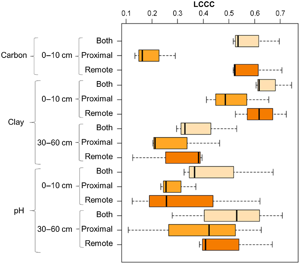
Fig. 4 and Table 3 show the LCCC values from the LOSOCV procedure for all soil properties, farms, depths, and data scenarios. Overall, the average results across all three farms showed that the models using both proximal and remote sensing data resulted in the best LCCC values. This was the case for all three soil properties (organic carbon, clay, and pH) in both the topsoil and subsoil. Using remote sensing data only produced the next best model predictions on average. Based on this study, using proximally-sensed data only produced, on average, the poorest model predictions.
Distribution of Lin’s concordance correlation coefficient (LCCC) across different farms for all models using leave-one-site-out cross-validation (LOSOCV).
| Soil property | Model | Depth (cm) | West Farm | North Farm | South Farm | Average | |
|---|---|---|---|---|---|---|---|
| Organic carbon (%) | Proximal and remote | 0–10 | 0.53 | 0.54 | 0.64 | 0.56 | |
| Proximal only | 0.16 | 0.29 | 0.13 | 0.20 | |||
| Remote only | 0.53 | 0.54 | 0.62 | 0.55 | |||
| Clay content (%) | Proximal and remote | 0–10 | 0.61 | 0.63 | 0.78 | 0.68 | |
| Proximal only | 0.41 | 0.49 | 0.66 | 0.52 | |||
| Remote only | 0.60 | 0.55 | 0.72 | 0.62 | |||
| Proximal and remote | 30–60 | 0.38 | 0.34 | 0.53 | 0.42 | ||
| Proximal only | 0.20 | 0.21 | 0.46 | 0.29 | |||
| Remote only | 0.38 | 0.12 | 0.44 | 0.31 | |||
| pH | Proximal and remote | 0–10 | 0.32 | 0.37 | 0.65 | 0.45 | |
| Proximal only | 0.24 | 0.25 | 0.37 | 0.29 | |||
| Remote only | 0.26 | 0.12 | 0.57 | 0.27 | |||
| Proximal and remote | 30–60 | 0.72 | 0.53 | 0.28 | 0.51 | ||
| Proximal only | 0.63 | 0.42 | 0.11 | 0.39 | |||
| Remote only | 0.67 | 0.41 | 0.39 | 0.46 |
*LCCC values are ranked by colour. Green, best; Orange, middle; Yellow, worst.
When looking at individual farm results, a similar pattern in the LCCC value for the combined models being superior to the remote or proximal only models was observed on all farms (Table 3). However, in the performance assessment between remote or proximal only models. On North Farm, the proximal models for soil pH at both depths, and subsoil clay content out-performed the remote only models. On South Farm, a similar result was observed for the subsoil clay content.
Table 4 shows the corresponding RMSE values for all models. Overall, the results reveal a similar pattern to the LCCC analysis, with the average RMSE of the combined proximal and remote sensing models from the three farms always making the most accurate predictions (lowest RMSE) and the remote only models generally the next best method. Again, when looking at individual farm results, a similar pattern in the RMSE value for the combined models being superior to the remote or proximal only models was observed on all farms. The RMSE assessment between remote or proximal only models also showed that on North Farm, the proximal models for soil pH at both depths, and subsoil clay content out-performed the remote only models. On South Farm, the same result was observed for the subsoil clay content
| Soil property | Model | Depth (cm) | West Farm | North Farm | South Farm | Average | |
|---|---|---|---|---|---|---|---|
| Organic carbon (%) | Proximal and remote | 0–10 | 0.29 | 0.11 | 0.28 | 0.23 | |
| Proximal only | 0.35 | 0.13 | 0.34 | 0.27 | |||
| Remote only | 0.30 | 0.11 | 0.28 | 0.23 | |||
| Clay content (%) | Proximal and remote | 0–10 | 5.25 | 5.60 | 3.86 | 4.85 | |
| Proximal only | 5.96 | 6.18 | 4.81 | 5.65 | |||
| Remote only | 5.23 | 5.99 | 4.49 | 5.24 | |||
| Proximal and remote | 30–60 | 10.27 | 3.72 | 8.21 | 7.40 | ||
| Proximal only | 10.94 | 3.75 | 8.53 | 7.74 | |||
| Remote only | 10.31 | 3.97 | 8.94 | 7.73 | |||
| pH | Proximal and remote | 0–10 | 0.46 | 0.46 | 0.58 | 0.50 | |
| Proximal only | 0.47 | 0.47 | 0.70 | 0.55 | |||
| Remote only | 0.47 | 0.51 | 0.66 | 0.55 | |||
| Proximal and remote | 30–60 | 0.77 | 0.34 | 0.41 | 0.51 | ||
| Proximal only | 0.86 | 0.37 | 0.44 | 0.56 | |||
| Remote only | 0.82 | 0.37 | 0.41 | 0.56 |
*LCCC values are ranked by colour. Green, best; Orange, middle; Yellow, worst.
Variables included in final model
After calculating the VIF to remove highly correlated predictors, and stepwise elimination to remove redundant predictors, the variables in the final model were recorded for all three data scenarios: proximal and remote (Table 5), proximal only (Table 6), and remote only (Table 7).
| Soil property | Depth interval (cm) | Farm | Proximal sensing data | Remote sensing data | ||||||||||||||||
|---|---|---|---|---|---|---|---|---|---|---|---|---|---|---|---|---|---|---|---|---|
| EM 50 cm | EM 150 cm | K | Th | U | DEM | TWI | K | Th | U | NDVI_5 | NDVI 50 | NDVI 95 | Blue | Red | SWIR1 | SWIR2 | ||||
| Carbon | 0–10 | West Farm | X | X | X | X | X | X | X | X | X | |||||||||
| Carbon | 0–10 | North Farm | X | X | X | X | X | X | X | |||||||||||
| Carbon | 0–10 | South Farm | X | X | X | X | X | X | X | X | ||||||||||
| Clay | 0–10 | West Farm | X | X | X | X | X | X | X | X | ||||||||||
| Clay | 0–10 | North Farm | X | X | X | X | X | |||||||||||||
| Clay | 0–10 | South Farm | X | X | X | |||||||||||||||
| pH | 0–10 | West Farm | X | X | X | X | X | |||||||||||||
| pH | 0–10 | North Farm | X | X | X | X | ||||||||||||||
| pH | 0–10 | South Farm | X | X | X | X | X | |||||||||||||
| Clay | 30–60 | West Farm | X | X | X | X | ||||||||||||||
| Clay | 30–60 | North Farm | X | X | X | X | X | X | X | |||||||||||
| Clay | 30–60 | South Farm | X | X | ||||||||||||||||
| pH | 30–60 | West Farm | X | X | X | X | X | X | ||||||||||||
| pH | 30–60 | North Farm | X | X | X | |||||||||||||||
| pH | 30–60 | South Farm | X | |||||||||||||||||
| Total occurrence | 1 | 6 | 10 | 1 | 3 | 3 | 6 | 4 | 5 | 4 | 7 | 2 | 7 | 7 | 1 | 8 | 2 | |||
EM, electromagnetic induction; DEM, digital elevation model; TWI, topographic wetness index; NIR, near infra-red; SWIR, shortwave infra-red; K, potassium; Th, thorium; U, uranium. Frequency of occurence, red = few; green = many.
| Soil property | Depth interval (cm) | Farm | Proximal sensing data | ||||
|---|---|---|---|---|---|---|---|
| EM 50 cm | EM 150 cm | K | U | ||||
| Carbon | 0–10 | West Farm | X | X | |||
| Carbon | 0–10 | North Farm | X | ||||
| Carbon | 0–10 | South Farm | X | ||||
| Clay | 0–10 | West Farm | X | X | X | ||
| Clay | 0–10 | North Farm | X | X | |||
| Clay | 0–10 | South Farm | X | X | |||
| pH | 0–10 | West Farm | X | ||||
| pH | 0–10 | North Farm | X | ||||
| pH | 0–10 | South Farm | X | ||||
| Clay | 30–60 | West Farm | X | ||||
| Clay | 30–60 | North Farm | X | ||||
| Clay | 30–60 | South Farm | X | ||||
| pH | 30–60 | West Farm | X | X | |||
| pH | 30–60 | North Farm | X | X | |||
| pH | 30–60 | South Farm | X | ||||
| Total occurrence | 5 | 5 | 10 | 2 | |||
Gamma radiometric Th and Total dose were not used in any of the models and so are not included in the Table.
EM, electromagnetic induction; K, potassium; U, uranium. Frequency of occurence, red = few; green = many.
| Soil property | Depth interval (cm) | Farm | Remote sensing data | ||||||||||||
|---|---|---|---|---|---|---|---|---|---|---|---|---|---|---|---|
| DEM | TWI | K | Th | U | NDVI 5 | NDVI 50 | NDVI 95 | Blue | Red | SWIR1 | SWIR2 | ||||
| Carbon | 0–10 | West Farm | X | X | X | X | X | X | X | X | |||||
| Carbon | 0–10 | North Farm | X | X | X | X | X | X | |||||||
| Carbon | 0–10 | South Farm | X | X | X | X | X | X | X | ||||||
| Clay | 0–10 | West Farm | X | X | X | X | X | X | |||||||
| Clay | 0–10 | North Farm | X | X | X | X | |||||||||
| Clay | 0–10 | South Farm | X | X | X | X | |||||||||
| pH | 0–10 | West Farm | X | X | X | X | X | ||||||||
| pH | 0–10 | North Farm | X | X | X | X | |||||||||
| pH | 0–10 | South Farm | X | X | X | X | |||||||||
| Clay | 30–60 | West Farm | X | X | X | X | X | ||||||||
| Clay | 30–60 | North Farm | X | X | X | ||||||||||
| Clay | 30–60 | South Farm | X | X | X | ||||||||||
| pH | 30–60 | West Farm | X | X | X | X | X | ||||||||
| pH | 30–60 | North Farm | X | X | X | ||||||||||
| pH | 30–60 | South Farm | X | X | X | ||||||||||
| Total occurrence | 3 | 5 | 5 | 4 | 8 | 8 | 6 | 7 | 11 | 1 | 8 | 4 | |||
EM, electromagnetic induction; DEM, digital elevation model; TWI, topographic wetness index; NIR, near infra-red; SWIR, shortwave infra-red; K, potassium; Th, thorium; U, uranium. Frequency of occurence, red = few; green = many.
Table 5 shows the variables included in the final model for each farm, soil property, and depth for the model where proximal and remote sensing data was available. Overall, proximally-sensed gamma radiometrics potassium was the most included of all variables in the study, being included in 10 of the 15 combined models. The EM data (150 cm) was the next most included proximally-sensed variable, being in six of the 15 combined models.
In terms of the remotely-sensed data, it was clear that the variables based on satellite imagery (NDVI and bare earth) were the most useful. In particular, the SWIR1 band from the barest earth Landsat imagery was the variable most included in the combined models (eight times). This was followed by the BE blue band, and NDVI 5th and 95th percentile (seven times each). This suggests that remotely-sensed imagery of crop biomass and bare soil can represent the variation in these important soil properties well on these farms. Further, the long-term NDVI imagery used here likely represents the whole soil profile as crop roots typically explore the upper metre of the soil profile. In contrast, the bare soil products likely represents the surface soil, which may or may not be related to the subsoil.
Variables that were not included in any of the combined models were the BE green and NIR band, and the total dose from both the proximal and remote gamma radiometric sensor (not shown in table). Other remotely-sensed variables that were rarely used in models were the BE red and SWIR2 band, NDVI 50th, and DEM. For proximally-sensed variables, EM (50 cm) was only included in one model. While thorium and uranium were often not included in models, this data was only available at one farm so this must be taken into account. Overall, only three of the 15 models used no proximally-sensed data, suggesting that proximal sensing provides considerable value when added to remote sensing data.
Table 6 also shows that gamma radiometrics potassium was the most included of all variables in the proximal sensing only data scenario models, being included in 10 of the 15 models. Both EM data layers (50 cm; 150 cm) were included five times each, but never in the same model. This suggests that these variables provide very similar information, and it is well known the EM at different depths are highly correlated. Although only available at one farm (West Farm), of the other proximally-sensed gamma radiometrics variables only U appeared in any models (two out of five).
Table 7 revealed a pattern of variable inclusion in the remote only models that was similar to that shown in the combined models (Table 5). Overall, the BE and satellite imagery variables were again predominant. The most included variable was the BE blue band (11 of the 15 models), followed by BE SWIR1 and NDVI 5th (eight times), and NDVI 95th (seven times). The airborne gamma radiometrics variables (especially U) were included in more models for the remote sensing only scenario than the combined models, likely because the proximally-sensed gamma data was not included. While the airborne, and ground-based gamma radiometrics are collected at very different spatial resolutions (100 m and 10 m, respectively), they would still represent the same broad patterns across fields and farms. The variables not included in any models were again the BE green and NIR bands, and the total dose from the airborne gamma radiometric sensor, similarly to the combined sensing data scenario.
Discussion
It is not unexpected that using both proximal and remote sensing data for modelling soil properties was found to generally result in the best model predictions. Variation in soil is driven by a number of different factors and their interaction. This can be described by the Scorpan framework (McBratney et al. 2003), and several of these factors are represented by the covariates used in this study. For example, the NDVI variables represent crop biomass, and therefore the vegetation variable (organisms, o), the elevation data reflects the relief variable (r), and the gamma radiometrics data represents the parent material variable (p). It is therefore logical that the proximal and remote data scenario produces the best model predictions as there is a larger suite of variables that describe the variation of soil.
While proximal sensing data has been seen as the ‘gold standard’ for within-field digital soil mapping (SPAA 2022), there are some other important reasons that may explain why the proximal sensing data only scenario generally produced the poorest predictions in this study. Proximal sensing data, such as soil ECa from an EMI instrument can identify within-field soil type variability well, however, when aggregating several fields together there are some limitations. Differences in management between fields can result in considerable differences in some soil properties, such as the soil moisture levels. This can lead to stark differences in absolute ECa values between fields, which is not driven by changes in soil type. This exaggerated extent of variability across the site reduces its usefulness as a covariate for modelling other soil properties. Many remote sensing variables do not suffer from the same problems, for example, the sensing of elevation and airborne gamma radiometrics are largely unaffected by agricultural management. It would be expected that if the focus of the study was on mapping individual fields under these different data scenarios that the proximal sensing only scenario would produce improved results from those observed in the current study.
Overall, the quality of the model predictions in this study varies considerably (Fig. 3, Table 3), and this is expected due to the differences in soil properties, depths, farms, and data scenarios. Although direct comparisons to results from other studies must be done with caution, the LCCC values from the LOSOCV procedure were similar to other published studies for clay content (Zhao et al. 2022), pH (Filippi et al. 2019b), and organic carbon (Wang et al. 2022).
The proximally-sensed predictor that was commonly identified as an important predictor across various farms, soil properties, and depths was the gamma radiometrics potassium. Compared to EM instruments, ground-based gamma sensors are relatively rare. To the best of our knowledge, only a few sensors are operational in Australia. Gamma potassium is known to be related to variation in soil type, parent material, and texture (Reinhardt and Herrmann 2019), so it is logical that this was identified as an important predictor for soil pH, clay content, and organic carbon. It is also known to be less impacted by differences in soil moisture compared to EM instruments (Whelan and Taylor 2013), which could also explain why it was identified as important when mapping across multiple agricultural fields in this study. The soil ECa data was identified as important for models in the proximal and remote data scenario (seven of 15 models), and the proximal only data scenario (10 of 15 models). Soil ECa data collected from EM instruments is very common worldwide, and it is well known that this data can be correlated to soil texture, moisture content, and overall soil fertility when salinity is not a dominant issue (Whelan and Taylor 2013).
While EM and gamma radiometric proximal sensors were used in the study due to prevalence of the sensors and data availability, there are also other on-the-go proximal sensors available to use in digital soil mapping on-farm. In particular, Veris Technologies have a suite of soil sensors available that utilise electrochemical sensors for on-the-go pH measurement, and visible and near-infrared (Vis-NIR) sensors to infer carbon and organic matter content of soils (Viscarra Rossel and Lobsey 2016). In the current study, the results showed that the average predictions of topsoil carbon were poor for the proximal only data scenario (Fig. 4). It could be envisioned that including data from these on-the-go Vis-NIR sensors would improve these predictions. The inclusion of some of these other proximal sensors should be considered in future research.
The BE and NDVI variables derived from satellite imagery were the variables that stood out in terms of their inclusion in models. The different percentiles (5th, 50th, 95th) of NDVI from 2000 to 2020 used in this study represent long-term trends in crop biomass and therefore production. Variation in crop production is linked to soil variability, particularly the soil properties modelled in the current study, which are important drivers of production. The BE imagery product based on the Landsat 5, 7 and 8 satellites (Roberts et al. 2019) proved important for modelling soil pH, clay content, and organic carbon. In particular, the blue band and SWIR1 band were prevalent in many models. The SWIR1 band, which covers wavelengths 1.55–1.75 μm for Landsat 5 and 7, and 1.57–1.65 μm for Landsat 8, is useful in discriminating the moisture content, and therefore water holding capacity of topsoil (Tian and Philpot 2015). Moisture content can be related to other soil properties, such as clay content. This could explain why the SWIR1 band was included in 8 of the 12 soil clay content models for the proximal and remote, and remote only data scenarios (Tables 5 and 7). The blue band, which covers 0.45–0.52 μm for Landsat 5 and 7, and 0.45–0.51 μm for Landsat 8, is known to help distinguish soil from vegetation. However, it is likely that the blue band is picking up differences in soil colour, which can be well related to the soil properties modelled in this study (Zhang et al. 2023).
Airborne gamma is commonly used in many Australian DSM studies at the national (Viscarra Rossel et al. 2015), regional (Pozza et al. 2022), and farm level (Filippi et al. 2019b). This gamma data has proven useful in modelling the variation in several soil properties. However, this study shows that satellite-derived sensor data (from the visible and near-infrared parts of the electromagnetic spectrum) of crops/plants and soil are also highly valuable in representing within-field and farm variability of important soil properties.
The increasing quantity of remote sensing and satellite imagery presents an invaluable opportunity for digital soil assessment. The accessibility of this data is improving considerably with platforms such as Google Earth Engine (Gorelick et al. 2017), and the quality is also rising. For example, the Sentinel 2 satellites can capture imagery at 10–20 m resolution, and includes a suite of bands in crucial parts of the electromagnetic spectrum (e.g. red edge). While many DSM studies have used satellite imagery as a covariate, there can be considerable differences in the type of imagery and the processing implemented. For example, some studies use a single-day remotely-sensed satellite image (Mirzaee et al. 2016), whereas others use multitemporal satellite images (Pozza et al. 2022). Many things need to be considered when processing satellite data for use as a covariate. Some of the primary factors are the satellite system (e.g. Landsat 8 or Sentinel 2), the time period (e.g. single image or some statistic of a collection of images), and the band or spectral index to select. These decisions can be made based on the specific goals of the study, but can result in an overwhelming amount of options.
In contrast, the BE imagery (Roberts et al. 2019) is a downloadable product, and does not require the same processing and decisions as the NDVI variables used in this study. This makes it much easier to use, and also more reproducible and accessible. These freely available products present a great opportunity for creating farm-scale digital soil maps for consultants and service providers.
Conclusions
This study assessed the value of using proximal and remote sensing data for mapping three different soil properties (organic carbon, clay, and pH), at two depths, and across multiple fields for three farms in different biogeographical locations across Australia. Three different data scenarios were considered: (1) using proximal sensing data only; (2) using remote sensing data only; and (3) using a combination of proximal and remote sensing. The results showed that using a combination of both proximal and remote sensing data resulted in the best predictions. Using remote sensing data only generally led to better predictions than proximal sensing data only. One possible reason for this is that soil variation is driven by a number of factors (e.g. organisms/vegetation, relief, parent material), and there is a larger and more diverse suite of remotely-sensed variables that can be used to represent these factors. Another thing to consider is that proximal sensing data is often affected by differences in management between fields, and combining data across multiple fields as we have done in this study may impact the value of this. Nonetheless, it was found that the proximally-sensed gamma radiometrics potassium was the most widely used of all the available variables for the proximal and remote data scenario. The remote sensing variables based on satellite imagery (NDVI and BE) were the standout predictors for many of the models in the data scenarios that included remote sensing data. This demonstrates that remotely-sensed imagery of crop/plant biomass and bare soil can represent the variation in important soil properties well. In particular, the BE imagery product presents a great opportunity for improving farm-scale digital soil mapping in Australia as it is also free and easily accessible as a downloadable product. Overall, this study shows that combining freely available and fine-scale remotely-sensed products to proximally-sensed data leads to more accurate farm-scale soil property maps that could inform important management decisions.
Data availability
The data that support this study cannot be publicly shared due to privacy reasons and may be shared upon reasonable request to the corresponding author if appropriate.
Conflicts of interest
Professor Thomas Bishop is an Editor of Soil Research but was blinded from the peer review process for this paper. The authors declare no other conflicts of interest.
Declaration of funding
This research was partly funded by the Grains Research and Development Corporation (GRDC).
Acknowledgements
The authors acknowledge Precision Cropping Technologies (PCT) for collecting the on-farm data, and the farms for collaborating and sharing data for this project.
References
Arrouays D, Lagacherie P, Hartemink AE (2017) Digital soil mapping across the globe. Geoderma Regional 9, 1-4.
| Crossref | Google Scholar |
CSIRO (2023) CSIRO data access portal. Available at https://data.csiro.au/ [Retrieved 8 June 2023]
Department of Finance, Services and Innovation (2023) NSW foundation spatial data framework-elevation and depth-digital elevation model. Available at https://data.nsw.gov.au/data/dataset/8f73f5ca-4f7f-4707-bfe2-0efbb9027107 [Retrieved 8 June 2023]
Farr TG, Rosen PA, Caro E, Crippen R, Duren R, Hensley S, Kobrick M, Paller M, Rodriguez E, Roth L, Seal D, Shaffer S, Shimada J, Umland J, Werner M, Oskin M, Burbank D, Alsdorf D (2007) The shuttle radar topography mission. Reviews of Geophysics 45, RG2004.
| Crossref | Google Scholar |
Filippi P, Jones EJ, Wimalathunge NS, Somarathna PDSN, Pozza LE, Ugbaje SU, Jephcott TG, Paterson SE, Whelan BM, Bishop TFA (2019a) An approach to forecast grain crop yield using multi-layered, multi-farm data sets and machine learning. Precision Agriculture 20, 1015-1029.
| Crossref | Google Scholar |
Filippi P, Jones EJ, Ginns BJ, Whelan BM, Roth GW, Bishop TFA (2019b) Mapping the depth-to-soil pH constraint, and the relationship with cotton and grain yield at the within-field scale. Agronomy 9, 251.
| Crossref | Google Scholar |
Gorelick N, Hancher M, Dixon M, Ilyushchenko S, Thau D, Moore R (2017) Google earth engine: planetary-scale geospatial analysis for everyone. Remote Sensing of Environment 202, 18-27.
| Crossref | Google Scholar |
Grunwald S, Thompson JA, Boettinger JL (2011) Digital soil mapping and modeling at continental scales: finding solutions for global issues. Soil Science Society of America Journal 75, 1201-1213.
| Crossref | Google Scholar |
Han SY, Filippi P, Singh K, Whelan BM, Bishop TFA (2022) Assessment of global, national and regional-level digital soil mapping products at different spatial supports. European Journal of Soil Science 73, e13300.
| Crossref | Google Scholar |
Lark RM, Cullis BR, Welham SJ (2006) On spatial prediction of soil properties in the presence of a spatial trend: the empirical best linear unbiased predictor (E-BLUP) with REML. European Journal of Soil Science 57, 787-799.
| Crossref | Google Scholar |
Liu M, Hu S, Ge Y, Heuvelink GBM, Ren Z, Huang X (2021) Using multiple linear regression and random forests to identify spatial poverty determinants in rural China. Spatial Statistics 42, 100461.
| Crossref | Google Scholar |
McBratney AB, Mendonça Santos ML, Minasny B (2003) On digital soil mapping. Geoderma 117, 3-52.
| Crossref | Google Scholar |
McBratney A, de Gruijter J, Bryce A (2019) Pedometrics timeline. Geoderma 338, 568-575.
| Crossref | Google Scholar |
McMillen DP (2010) Issues in spatial data analysis. Journal of Regional Science 50, 119-141.
| Crossref | Google Scholar |
Minty B, Franklin R, Milligan P, Richardson M, Wilford J (2009) The radiometric map of Australia. Exploration Geophysics 40, 325-333.
| Crossref | Google Scholar |
Mirzaee S, Ghorbani-Dashtaki S, Mohammadi J, Asadi H, Asadzadeh F (2016) Spatial variability of soil organic matter using remote sensing data. Catena 145, 118-127.
| Crossref | Google Scholar |
Pozza LE, Filippi P, Whelan B, Wimalathunge NS, Jones EJ, Bishop TFA (2022) Depth to sodicity constraint mapping of the Murray-Darling Basin, Australia. Geoderma 428, 116181.
| Crossref | Google Scholar |
R Core Team (2020) ‘R: a language and environment for statistical computing.’ (R Foundation for Statistical Computing: Vienna, Austria) Available at https://www.R-project.org/
Reinhardt N, Herrmann L (2019) Gamma-ray spectrometry as versatile tool in soil science: a critical review. Journal of Plant Nutrition and Soil Science 182, 9-27.
| Crossref | Google Scholar |
Roberts D, Wilford J, Ghattas O (2019) Exposed soil and mineral map of the Australian continent revealing the land at its barest. Nature Communications 10, 5297.
| Crossref | Google Scholar |
Searle R, McBratney A, Grundy M, Kidd D, Malone B, Arrouays D, Stockman U, Zund P, Wilson P, Wilford J, Van Gool D, et al. (2021) Digital soil mapping and assessment for Australia and beyond: a propitious future. Geoderma Regional 24, e00359.
| Crossref | Google Scholar |
Tian J, Philpot WD (2015) Relationship between surface soil water content, evaporation rate, and water absorption band depths in SWIR reflectance spectra. Remote Sensing of Environment 169, 280-289.
| Crossref | Google Scholar |
Tilse M, Stockmann U, Filippi P (2023) Proximal soil sensing in the field. In ‘Encyclopedia of soils in the environment’. (Eds MJ Goss, M Oliver) pp. 579–589. (Elsevier) doi:10.1016/B978-0-12-822974-3.00188-9
Viscarra Rossel R, Lobsey C (2016) Scoping review of proximal soil sensors for grain growing. p. 52. (CSIRO) Available at https://doi.org/10.13140/RG.2.2.34785.51049
Viscarra Rossel RA, Chen C, Grundy MJ, Searle R, Clifford D, Campbell PH (2015) The Australian three-dimensional soil grid: Australia’s contribution to the GlobalSoilMap project. Soil Research 53(8), 845-864.
| Crossref | Google Scholar |
Wang J, Zhao D, Zare E, Sefton M, Triantafilis J (2022) Unravelling drivers of field-scale digital mapping of topsoil organic carbon and its implications for nitrogen practices. Computers and Electronics in Agriculture 193, 106640.
| Crossref | Google Scholar |
Whelan B, Taylor J (2013) ‘Precision agriculture for grain production systems.’ (CSIRO) doi:10.1080/17538947.2013.817183
Zhang Y, Hartemink AE, Huang J, Minasny B (2023) Digital soil morphometrics. ln ‘Encyclopedia of Soils in the Environment’. 2nd edn. (Eds MJ Goss, M Oliver) pp. 568–578. (Academic Press) doi:10.1016/B978-0-12-822974-3.00008-2
Zhao D, Wang J, Zhao X, Triantafilis J (2022) Clay content mapping and uncertainty estimation using weighted model averaging. Catena 209, 105791.
| Crossref | Google Scholar |