

Estimating surrogates, utility graphs and indicator sets for soil capacity and security assessments using legacy data
Wartini Ng A * , Sandra J. Evangelista A , José Padarian A , Julio Pachon A , Tom O’Donoghue A , Peipei Xue A , Nicolas Francos A and Alex B. McBratney A
A
Abstract
Legacy data from prior studies enable preliminary analysis for soil security assessment which will inform future research questions.
This study aims to utilise the soil security assessment framework (SSAF) to evaluate the capacity of soil in fulfilling various roles and understand the underlying drivers.
The framework entails: (1) defining a combination of role(s) × dimension(s) and identifying a target indicator (a soil property that can be used to evaluate a particular role × dimension combination) or a surrogate indicator (an alternative indicator when there is not a clear target indicator); (2) transforming the indicator into a unitless score (ranging from 0 to 1) using a utility graph based on expert knowledge; (3) fitting the remaining soil properties (potential indicators) into utility graphs and weighing them using (a) ordination and (b) regression method. The application of this framework is demonstrated in evaluating two soil roles: nutrient storage and habitat for biodiversity (with pH and microbial DNA Shannon’s diversity index as surrogates, respectively) for an area in the lower Hunter Valley region, New South Wales, Australia.
The regression model provides utility estimates that were similar to those obtained from surrogates, in comparison to the utility derived from the ordination model.
This study provides a methodological pathway to examine the capacity and drivers of fulfilling different soil roles. The standardisation of this method opens the door to a complete quantification under the SSAF.
Indicators derived from a legacy dataset can be used for soil security assessment.
Keywords: habitat for biodiversity, indicator, indicator selection, legacy dataset, minimum dataset, nutrient storage, ordination, principal component analysis, regression, soil security assessment framework, surrogates, utility graphs.
Introduction
Soil is an essential natural resource for the existence of our life on the planet. Its significance extends beyond food production, as it provides a habitat for a vast range of biodiversity, acts as a carbon and nutrient store, and supports various life-sustaining functions. Various soil concepts have been developed since the early to the mid-twentieth century (Karlen et al. 2019; Evangelista et al. 2023a) which highlight the evolution of these concepts through time. All these concepts were aimed to raise awareness of the need to protect soil. Contemporary soil concepts such as soil health are described to be more holistic about the overall well-being of the soil environment; however, they often focus on the soil function to produce food and biomass. In order to perpetuate humanity and planetary functioning, there is a need to consider all of the soil security dimensions as described by Evangelista et al. (2023a, 2023b).
Soil security (McBratney et al. 2014) is an overarching concept that aims to protect the soil based on five dimensions (capacity, condition, capital, connectivity, and codification) and three different roles: its functions, services, and resilience to threats (Evangelista et al. 2023b). A full assessment will require multiple sub-assessments for each function, service, and threat. Through these roles and dimensions, the soil security concept encompasses soil health and soil quality, which correspond most closely with the dimensions of condition and capacity, respectively. Furthermore, broader evaluations of soil quality or health with respect to soil threats and other services has rarely been implemented (Bünemann et al. 2018).
Reviews of existing soil assessments (Bünemann et al. 2018), the history of soil assessments (Karlen et al. 2019), and future prospects of soil assessments (Lehmann et al. 2020) have been recently published. In this paper, we review six assessment frameworks to highlight differences in their approach and structure: the functional capability classification (FCC; Sanchez 2019), the environmental assessment of soil for monitoring (ENVASSO; Huber et al. 2008), soil management assessment framework (SMAF; Andrews et al. 2004), soil quality sssessment (SQAPP; Spiegel et al. 2015), the comprehensive assessment of soil health (CASH; Moebius-Clune et al. 2016), and the soil security assessment framework (SSAF; Evangelista et al. 2023a, 2023b).
A common factor for all assessment frameworks is the need to select soil indicators, defined as a collection of soil properties that have greatest sensitivity to changes in the assessment for a particular soil function, service and/or threat under a particular soil dimension. Indicators should integrate physical, chemical, and biological soil properties and processes (Doran and Parkin 1997) and whenever possible, be inexpensive and easy to measure to enable greater rates of sampling or monitoring (Schoenholtz et al. 2000). Prescriptive assessment frameworks such as the CASH, ESMAF, and SQAPP have selected indicators based on regional datasets from which indicators were narrowed down from a larger list created by expert knowledge. These frameworks have 18, ~14, and six indicators for the CASH, ESMAF, and SQAPP, respectively. However, the availability of indicators in prescriptive assessments may not be captured by existing datasets or legacy data, resulting in the need to gather new information, which may be time and cost intensive. By not utilising existing or legacy data, the ability to investigate soil security in the past is also hindered. Hence, there is a demand for an objective and adaptable framework, such as the SSAF, which is capable of utilising existing and legacy databases to derive insights into past soil security and inform future research.
The SSAF is more advanced than the other frameworks in the sense that it does not necessarily require a target indicator. If the target indicator has been independently measured, a utility graph (transformation of indicator values into utility scores) as a function of target indicator can be fitted. However, in the case where the target indicator is not available, a surrogate indicator can be nominated. The use of a surrogate has been adopted by various stakeholders, namely modellers, scientists, agriculturalists, and land managers; thus, total organic carbon can be used as a proxy for various soil processes, such as aggregate formation, water retention, and nutrient cycling. Utility score, usually represented on a common scale (0–1), explains the variation of relationships between the soil indicator and assessment for a particular soil role. In this paper, we investigate methods which build upon a standardised approach using an ordination method, such as principal component analysis (PCA) (Andrews and Carroll 2001; Andrews et al. 2002a, 2002b) and a regression method to quantitatively select and integrate indicators from existing and legacy datasets, enabling the derivation of soil security information. Such an objective and adaptable framework should also guide users on the integration of chosen indicators which serve as a crucial communication tool among stakeholders, allowing a comprehensive understanding of the underlying factors associated with each indicator.
Although soil provides humanity with many different roles, in this study, we will explore the use of the proposed framework on two case studies exploring different soil functions in the capacity dimension: habitat for biodiversity and store and regulator of nutrients. Biodiversity contributes to many important ecosystem functions (Wall et al. 2015; Guerra et al. 2020). Soil microbial biodiversity indicators may be especially important to understand changes in soil processes given their interaction with soil structure and their sensitivity to land management (Hartmann and Six 2023). Furthermore, soil also serves as a reservoir of nutrients, providing essential macro- and micronutrients to sustain plant and animal growth and contribute to a range of environmental services such as climate regulation through the cycling of nutrients. The decomposition of various sources in the soil (e.g. organic matter) and weathering of parent material (e.g. minerals) contribute to elemental storage, and the cycling of nutrients is regulated through the transformation and translocation by various soil properties (e.g. environmental factors). A nutrient imbalance in soils has been increasingly considered a primary limiting factor of agricultural productivity in Africa and India (Pathak 2010; Stewart et al. 2020). Where soil infertility is recognised as poor soil quality (capacity) and in poor health (condition), it poses a great threat to soil security, thus exacerbating global challenges.
Soil assessment frameworks
The SSAF, a newly developed comprehensive framework, offers a cohesive approach to understanding soils, guiding surrogate selections for soil functions, services, and threats (Evangelista et al. 2023b). It encompasses five key dimensions: capacity, condition, capital, connectivity, and codification, enabling a holistic perspective on soil analysis. Following this concept allows us to acknowledge gaps in our understanding about what may be impacting a site’s soil security. Like the SMAF and CASH, the SSAF follows three steps: (1) selecting indicators for a management goal from the existing dataset; (2) interpreting indicators by transforming the selected indicators into a unitless value or score; and (3) where appropriate, integrating the scores into a single value. The SSAF and SMAF do not prescribe indicators to use or the type of integration, recognising that there are an increasing number of algorithms that may be used (Evangelista et al. 2023b). Although the SSAF is not prescriptive on the indicators to use, its all-inclusivity provides guidance as to what indicators to seek and how to connect different aspects of soil security together.
The fertility capability classification (FCC), created in 1975 to characterise plant growth limitations in the tropics due to its focus on the function of soil as a producer of food and biomass, now describes soil characteristics relevant to both agronomic and ecologic disciplines across the world (Sanchez 2019). This framework is different from the others discussed by its focus on quantifying soil attributes of the top 50 cm considered to be inherent, or not easily changed within a span of years to decades (Sanchez et al. 2003), and being highly relevant to understanding soil security, such as soils with high phosphorous sorption capabilities, high leaching potential, and sodic soils. A set of 31 binary indicators, presence or absence, describing 20 different soil attributes along with a textural description of topsoil and subsoil have been developed over 40 years from expert knowledge. Within the SSAF framework, these inherent indicators would be classified under the capacity dimension and distinguished by their connection to a soil function of food and biomass production.
In Europe, as part of the ENVASSO project, 27 soil indicators were identified from an initial selection of 290 to protect soils in the EU (Huber et al. 2008). Potential indicators (PI) were obtained from literature review; indicators were then linked to nine soil threats and key issues within the respective threat, and final indicators chosen by expert judgment. This framework is slightly different from the other frameworks mentioned due to its distinctiveness in choosing a more specific set of indicators comprising three indicators per threat assessed, called TOP3. These indicators were carefully selected based on expert insights, considering their alignment with EU policy objectives. Similarly, the SSAF also considers policy aspect within its codification dimension which can be evaluated across various roles.
The SMAF, introduced by Andrews et al. (2004), is a site-specific tool designed to assess and evaluate soil management practices, particularly in relation to soil quality (capacity). As described above, the SMAF introduced the three steps used in the SSAF and CASH. This flexible framework is not prescriptive; however, the authors have identified over 70 PI and developed scoring functions for over a dozen along with a protocol to create the scoring functions (Wienhold et al. 2009). The CASH framework was derived based on the SMAF (Moebius-Clune et al. 2016) and focused on overall soil health (condition) within agricultural systems through the combined use of a predefined set of 18–25 indicators (from basic to NRCS-216 level of soil health analysis) covering the physical, biological, and chemical soil properties. It is then transformed into a score following the method described in Andrews et al. (2004), with value ranging from 0 to 100, with a higher number indicating optimum or near optimum condition. The scoring functions are texture based but undergoing efforts to account for texture, suborder classes, and mean annual temperature and precipitation in the continental USA using the Soil Health Assessment Protocol and Evaluation (SHAPE; Nunes et al. 2021). The overall soil health index (SHI) is determined by taking the average of all indicators measured. Within the SSAF, these indicators which are sensitive to anthropogenic activities would be classified under the condition dimension. In the SSAF, condition indicators of a target are compared to an area with similar pedogenic origin but minimal anthropogenic impact. Pedogenon can be defined as a conceptual soil taxon created from a regionalised set of quantitative state variables representing the soil-forming factors for a given reference time (Román Dobarco et al. 2021).
The SQAPP was formed to account for the impact that agricultural land management has had on soil properties and functions to be accessed via a mobile application. Six soil quality indicators were ultimately chosen based on work by Spiegel et al. (2015) and Bünemann et al. (2018): soil organic matter (SOM) content, pH, aggregate stability, water-holding capacity, and number of earthworms. The indicators are meant to show gradual soil quality and fertility changes in a span of more than 5 years, be soil and site specific, related to potential changes in soil functions and threats, and be easily interpretable by farm and land managers (Bai et al. 2018). Indicators in the SQAPP are presented as response ratios (RR) where the treatments were paired; for example, crop rotation versus monoculture. Rather than providing an integrating score, the SQAPP presents the results in radar charts, consistent with the idea that each indicator needs to be looked at individually. With the use of an application, this framework is focused on improving the connectivity different land managers have with their soil; connectivity is another dimension recognised under the SSAF and under which SQAPP data can be used to inform researchers and legislators.
The uniqueness of the SSAF lies in its ability to encompass multifaceted aspects of soil security. Unlike its counterpart’s framework that focuses solely on a certain dimension, the SSAF adopts a holistic approach. In the next section, methods implemented in the SSAF framework will be described.
The aims of this paper are to:
Present a new approach by identifying surrogate indicator and fitting a utility graph,
Develop a workflow of screening for potential indicators and estimating their utility using: (a) ordination, and (b) regression methods, and
Investigate two case studies testing the proposed approach and making a brief comparison of the two different methods mentioned above.
Methods
Study area and dataset
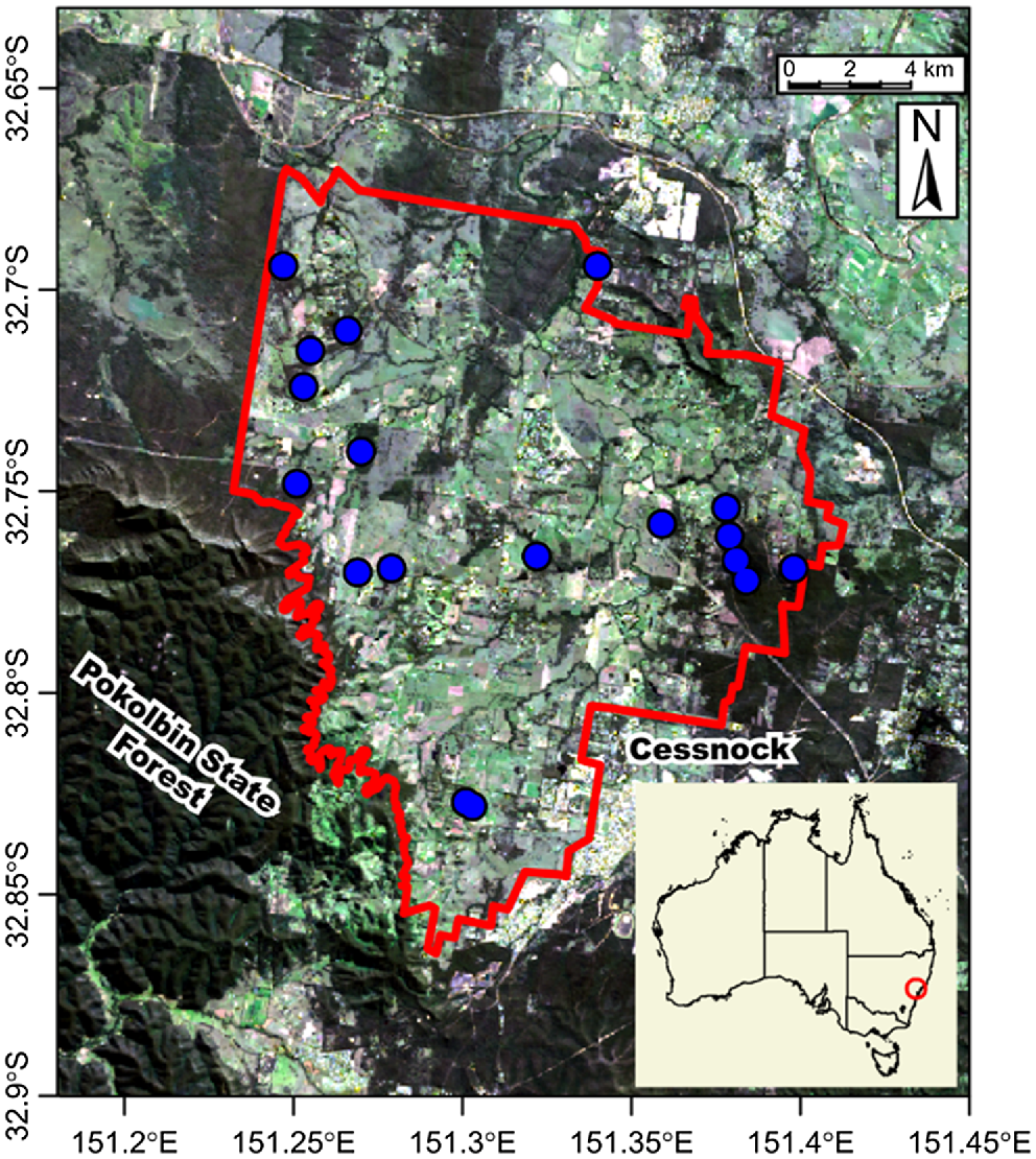
The study area is located in the Hunter Wine Country Private Irrigation District (HWCPID), New South Wales, Australia, covering an area of approximately 220 km2 (Fig. 1). The climate in this region is temperate, with annual rainfall of 750 mm and seasonal temperature ranging from 4 to 30°C. The soil samples were collected in October 2019 across from the native forests belonging to three dominant soil orders (Chromosols, Kurosols, and Calcarosols) according to the Australian Soil Classification system (ASC). Following the soil map developed by Huang et al. (2018), the soil types within the study area can be mainly categorised into: Brown Chromosol, Brown and Red Kurosol, and Red Calcarosol.
Location of the sampling points for case studies within the Hunter Wine Country Private Irrigation District (HWCPID) shown in the red border on a May 2023 Landsat-9 image courtesy of the U.S. Geological Survey. The inset shows the location of the HWCPID within Australia. The Australian map shows territory and state divisions.
The dataset used corresponds to a subset of the data collected for a previous study by Xue et al. (2023). Eighteen sampling sites were selected, in which three soil cores (10 cm diameter) were collected as replicates. Within each soil core, the soil samples were collected across three depths (5–15 cm, 45–55 cm, and 90–100 cm) from the soil surface to 1 m depth.
A series of soil analyses were performed. For each soil sample, half was air-dried and ground to <2 mm prior to analysis through a commercial laboratory for 16 physico-chemical properties following methods described in Rayment and Lyons (2011). Analysis measured include (with method codes from Rayment and Lyons 2011): pH (1:5 CaCl2) – 4B2; organic carbon (OC; Walkley and Black 1934) – 6A1; total nitrogen (N) (combustion) – 7A5; electrical conductivity (EC; 1:5 water) – 3A1; exchangeable aluminium (exch. Al; 1 M KCl) – 15G1; exchangeable sodium (exch. Na; 1 M NH₄CH₃CO₂) – 15D3; cation exchange capacity (CEC) – 15J1; and total (acid digest) phosphorus (P), copper (Cu), calcium (Ca), magnesium (Mg), manganese (Mn), nickel (Ni), potassium (K), sulfur (S), and zinc (Zn) – 17B1. Any elemental values that fall below the detection limit were recorded as zero (absent). The other half of the soil sample was subsampled and stored in the freezer (~ −20°C) before soil DNA extraction. Soil DNA was extracted from 10 g soil following the protocol provided in the supplementary (Supplementary A) in Metagen Lab®. DNA concentration was quantified using the Quantifluor dsDNA system (Promega, WI, USA). Primer sets of ArBa515F/Arch806R were used for polymerase chain reaction amplifications. Amplicon pyrosequencing was then sequenced on the Illumina MiSeq platform (PE 300). The sequencing data was filtered and merged using USEARCH (v.7.0) (Edgar 2010) and the merged sequences were clustered into operational taxonomic units (OTUs) by UPARSE (Edgar 2013). Soil microbial alpha diversity was calculated by Shannon index using the rarefied OTU table with vegan package (v2.6.2; Dixon 2003). For detailed information about the methods, we refer the reader to the original study (Xue et al. 2023). Two examples from this dataset are presented to exemplify the utilisation of the SSAF.
SSAF procedure
To evaluate the soil security assessment, a combination of a single or multiple roles (function, service, or threat) along with a single or multiple dimensions per role (capacity, condition, capital, connectivity, and codification) needs to be identified, as outlined in the SSAF (Evangelista et al. 2023b).
Once the combination of role(s) and dimension(s) have been identified, the SSAF procedure shown in Fig. 2 can be undertaken.
Identify a surrogate indicator,
Transform the surrogate indicator to a utility score using the utility graph,
Transform the remaining indicators (potential indicators) to utility scores by fitting them against the utility graphs of the surrogate indicator and screen indicators fit using an F-test,
Weigh these screened potential indicators using:
The subsequent sections will elaborate on each step of the SSAF procedure.
Conceptual framework for proposed soil security assessment framework (SSAF) method to create minimum dataset using (IVa) ordination and regression (IVb) method. U* is the utility of the transformed surrogate, PI is potential indicators, is the utility of F-test screened potential indicators (SPI), and is the estimated utility. The obelisk (†) shows that the choice of regression will impact the outputs. In the case of neural networks, is the main output.
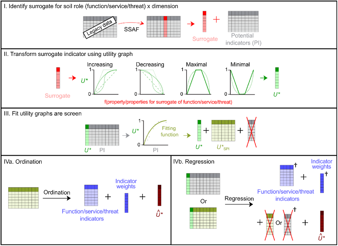
Although it is vital to measure soil security as a whole, the assessment can be done through a combination of role and dimension depending on the goals set by the stakeholders. In most cases, a directly measurable target indicator that encapsulates a particular role × dimension pairing is rarely available and expert opinion is leveraged to infer a suitable surrogate indicator (Fig. 2 – section I).
To facilitate interpretation and possible integration of role × dimension combinations, the variable or surrogate indicator needs to be transformed into an ordinal or unitless score using a utility graph as discussed by Evangelista et al. (2023a). A utility graph represents the relationship between the values of the surrogate indicator on the x-axis and the utility of role × dimension combination (U*) (Fig. 2 – section II).
Once a surrogate for the role × dimension combination is chosen, the remaining soil properties in the dataset are referred to as PI.
Each PI is mapped against U* across various possible curves to identify the best fit, be it linear, quadratic, exponential, or logarithmic. Subsequently, an F-test is applied to each fit to determine its statistical significance, with a P-value threshold set at less than 0.05. Indicators that demonstrate a significant correlation are retained, hereon referred to as screened potential indicators (SPI). This method is similar to the non-parametric approach described by Andrews and Carroll (2001). Feature selection based solely on numerical reasoning is regularly done to make the models more robust, handle multicollinearity, reduce overfitting, and increase computer efficiency.
Two of the most commonly used methods of weighting PI were explored: ordination and regression.
Principal component analysis is used as the ordination technique to assign weights to the PI, following the methods described in Andrews and Carroll (2001), Andrews et al. (2002a), and Andrews et al. (2002b) with slight modifications (Fig. 2 – section IVa). First, the transformed was used instead of using the SPI directly, and also normalised the final weights to add up to one. Details of this method are described in Fig. 3.
Conceptual framework using PCA for dimension reduction with steps proposed in this paper indicated by an obelisk (†). PC is the principal component, is the utility of F-test screened potential indicators, Wn = % variation explained by nth selected PC/∑ % variation explained by all selected PCs.
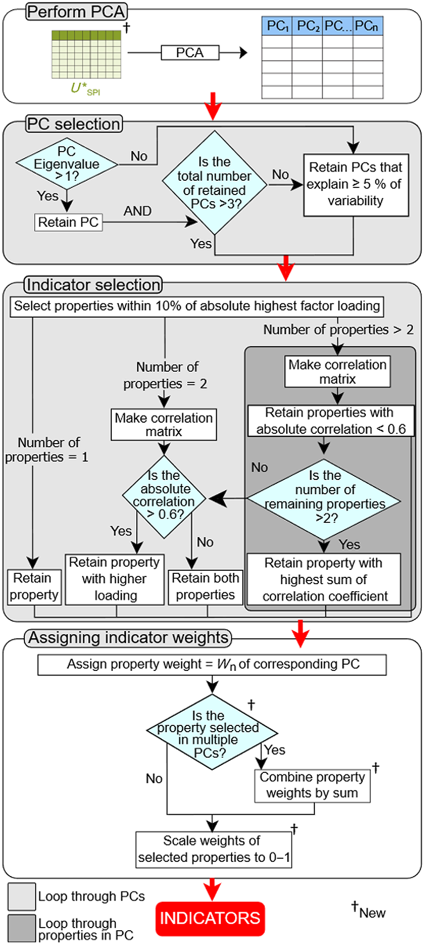
In short, the principal components (PC) with large eigenvalues (≥1) were selected (Andrews and Carroll 2001; Andrews et al. 2002a, 2002b). However, if less than three PC had eigenvalues of ≥1, another PC that explained ≥5% variations within the dataset was also included (Andrews et al. 2002a). Within a particular PC, any SPI that had absolute values of loadings within the range of 10% of the highest factor loading were kept. The following steps depend on the number of identified properties:
If there is only one property identified, the property is included in the selected indicators.
If there are two properties identified, a correlation analysis is performed. If the properties are uncorrelated (|r| < 0.6), both properties are included in the selected indicators. (Andrews et al. 2002a). However, if both properties are correlated, the property that has the higher loading is included.
If there are more than two properties identified, a correlation analysis is also performed. Properties that are uncorrelated (|r| < 0.6) are included in the selected indicators. From the correlated properties, if only two are left, the one with the higher loading is included. If more than two are left, only the property that has the highest absolute values of sum of correlation coefficient is included.
Each selected indicator has a weight corresponding to the PC from which it was selected. The weights for each PC can be obtained by dividing the percent of variation explained by the PC by the sum of percent variation explained of all selected PC (eigenvalues ≥ 1). Note that an indicator can be selected in more than one PC. This happens when there is a non-linear relationship with the rest of the properties and a single PC is not capable of capturing all the variation. We could not find examples of this in previous studies. Additionally, unlike Andrews et al. (2002b), the final weights were normalised to sum to one, instead of having an unbounded score, greater than one.
The final estimated utility of a role, () then corresponds to the weighted sum of all the selected indicators (Eqn 1).
Where is the estimated utility of soil for the given role, Wi is the weight of indicator i, and is the utility of indicator i to support a particular certain role.
In the ordination case, obtaining best-fit curves for each of the indicators corresponds to generating a series of univariate regressions to predict the utility. Each indicator can then generate its own estimate of the utility and all the estimates are combined using a weighted average where the weights are obtained by PCA. This approach helps to rationalise the effect of each individual indicator but disregards interactions between indicators.
To overcome the limitations of the ordination method, the use of multivariate regression approach using a neural networks model is explored. In this context, neural networks present two desirable properties: (a) they can fit non-linear relationships between indicators and the utility, and (b) they can also consider interactions between indicators (Fig. 2 – section IVb).
Here, two types of regression methods were explored: (1) with the complete set of PI and (2) only using indicators selected by the F-test screening. Since the number of observations was limited, a small neural network architecture was utilised with two hidden-layers and tanh activation functions. The number of neurons was set depending on the number of inputs, with 15 and five neurons for the two hidden layers in the case of using the 16 PI and four or five, and two for the hidden layers in the case of only using selected indicators. For the output of the model, a sigmoid activation function, which limits the output to the 0–1 range, was used. The models were trained for 200 epochs, using a learning rate of 0.0005 and a batch size of 10 samples. The hyper-parameters were found using a grid search using two randomly selected sites as validation set. The model was also trained with early stopping in place to avoid overfitting.
In the case of regression, it is not always possible to obtain explicit weights for each indicator as in the case of ordination (PCA). If that is a priority, multiple linear regression can be utilised to obtain weights for each indicator. In the case of neural networks, the final estimated utility is predicted directly using the internal weights of the neurons which are adjusted during the training process.
Model evaluation
The performance of the ordination and regression model was evaluated using coefficient of determination (R2), and root mean square error (RMSE) based on the agreement of the estimated utility from the surrogates and those from PI and SPI. R2 represents the proportion of total variance in the target variable explained by the model. It assesses how well the utility is approximated by model predictions. RMSE utilises the square root of the sum of the squares of the residuals to evaluate the performance of the model, where it is adjusted by the number of observations. It describes how close the estimated utility from the model is to the observed utility from the surrogates.
Implementation
The data analyses were conducted in Python (v3.6.9; Python Software Foundation 2021) using packages from matplotlib (v3.6.2; Hunter 2007), statsmodels (v0.13.5; Seabold and Perktold 2010), scikit-learn (v1.2.0; Pedregosa et al. 2011), and Tensorflow (v2.4.1; Abadi et al. 2016).
Results
Case study 1. Function: a habitat for, and of, biodiversity
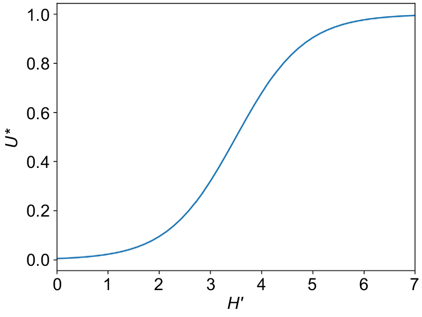
For this case study, Shannon diversity index (H′) is selected as the surrogate indicator. The Shannon index (Shannon 1948) is one of the popular metrics used in ecology. It’s based on Claude Shannon’s formula for entropy and estimates species diversity, which considers the number of species living in a habitat (richness) and their relative abundance (evenness).
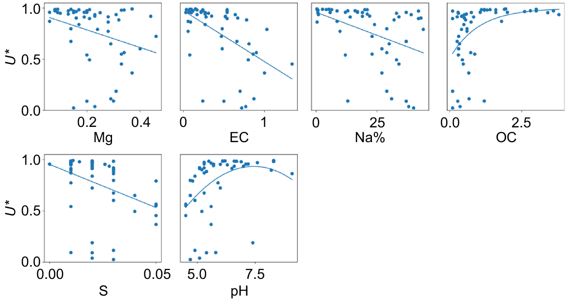
The utility graph of Shannon index shows increasing utility as the Shannon index increases, as a diverse microbial community is desired. It is also assumed that this relationship is sigmoidal, reflecting the idea that synergistic interactions between soil fauna improves the utility up to a certain point. Overall, the sigmoidal shape (Eqn 2) of our utility graph covers the range in our data and has the inflection point at the mid-point (Fig. 4).
After selection of the surrogate property, the remaining datasets are the PI. Upon screening with the F-test, only six models fit the population of their respective property well enough to be passed on to the next step: Mg, EC, exch. Na, OC, S, and pH (Fig. 5). The following variables were thus not part of the subsequent PCA: total N, P, Cu, Ca, Mn, Ni, K, and Zn, as well as exch. Al and CEC.
Out of the six SPI, Table 1 shows the PCA indicators selected for the utility of biodiversity, in decreasing order of importance: EC, OC, pH, and Mg. For this area, Na and S were highly correlated with the selected indicators, hence redundant to assess biodiversity.
| Property | |||||||
|---|---|---|---|---|---|---|---|
| Weight | 0.53 | 0.22 | 0.17 | 0.09 | – | – |
Overall, the PCA led to overestimation of low utility scores (Fig. 6d) of biodiversity with R2 = 0.35 and RMSE = 0.23. In the case of biodiversity, the final index can be obtained by the weighted sum of the indicators (Eqn 3):
Comparison of utility graphs (U*; blue circle) and predicted utility (; orange triangle) for soil as a habitat of biodiversity using (a) ordination by principal component analysis of screened potential indicators (SPI), (b) regression of all potential indicators (PI), and (c) regression of SPI. Model agreement between utility graphs and predicted utility from (d) principal component analysis of SPI, (e) regression of all PI, and (f) regression of SPI.
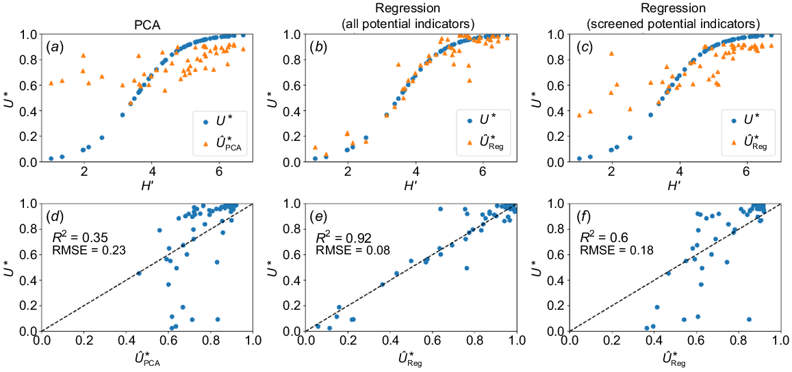
The regression case is more straightforward compared with the ordination method since the utility is predicted directly from the untransformed indicators. Both neural networks, outperformed the PCA method obtaining a R2 = 0.92 and RMSE = 0.08 when using all the PI (Fig. 6e) and an R2 = 0.6 and RMSE = 0.18 when only using the SPI (Fig. 6f).
To summarise all of the methods, the regression performed better than the ordination by PCA when estimating the utility (Fig. 6). The regression results highlight the ability to capture complex relationships and interactions which is reflected in the better performance. It also highlights the trade-off between performance and data requirements, which is a factor to consider when implementing the method in the future.
Case study 2. Function: a store and regulator of nutrients
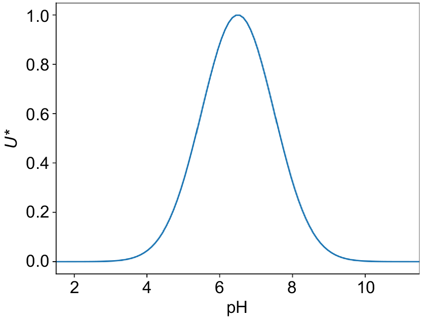
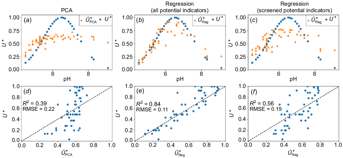
In this case study, pH was selected as the surrogate indicator to assess the ability of soil to store and regulate nutrients under the capacity dimension. It has been well researched that pH influences the availability of elements within the soil where many essential plant nutrients, contaminants, and cycles (i.e. nitrogen cycle, carbon cycle) are sensitive to pH changes. We acknowledge that pH can be considered both an indicator of capacity and condition since it has been extensively used to assess soil quality (capacity) and soil health (condition) (Karlen et al. 1992; Arshad and Martin 2002; Shukla et al. 2006; Allen et al. 2011). Though capacity refers to the inherent properties of soil, pH may still be employed as an indicator when referring to genosoils. With that, our data only included soils under native vegetation to represent this.
Most elements are plant available within a certain range around the pH of 7 while the same elements may become unavailable towards both extremes of the pH scale or become toxic at those pH extremes. As such, a maximal utility graph best describes the utility of pH. A Gaussian model was fitted with the parameters of μ = 6.5 and σ = 1. This produced a similar utility graph to the scoring function devised by Andrews et al. (2002b) (Fig. 7).
Upon screening with the F-test, only five models fit the population of their respective property well enough to be passed on to the next step: total N, exch. Al, EC, total S, and CEC (Fig. 8). The following variables were thus not part of the proceeding PCA: total OC, P, Cu, Ca, Mn, Ni, K, and Zn, as well as exch. Na.
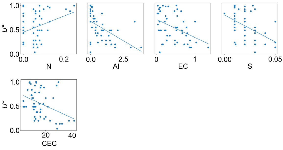
Out of the five SPI, Table 2 shows the PCA indicators selected for the utility of nutrient storage, in decreasing order of importance: S, Al, N, and CEC. For this area, EC is not an important factor for biodiversity.
| Property | ||||||
|---|---|---|---|---|---|---|
| Weight | 0.52 | 0.25 | 0.15 | 0.07 | – |
Overall, the PCA led to overestimation of the utility of nutrient storage and regulation at pH below 5.5, underestimation of the utility between 5.5 and 7.5, and overestimation of utility above 7 with R2 of 0.39 and RMSE of 0.22 (Fig. 9d).
Comparison of utility graphs (U*; blue circle) and predicted utility (; orange triangle) for soil as a store and regulator of nutrients using (a) principal component analysis of screened potential indicators (SPI), (b) regression of all potential indicators (PI), and (c) regression of SPI. Model agreement between utility graphs and predicted utility from (d) principal component analysis of SPI, (e) regression of all PI, (f) and regression of SPI.
Similar to the previous case study, the final index (Eqn 4) for nutrient cycling and storage can be obtained by the weighted sum of the indicators:
Similar to the previous case study, both neural networks outperformed the PCA method, obtaining an R2 of 0.84 and RMSE of 0.11 when using all the PI (Fig. 9e) and R2 of 0.56 and RMSE of 0.19 when only using the SPI (Fig. 9f).
Again, lower performance of the PCA ordination compared with the regression was observed, and the number of predictors playing an important role in the final performance, enforcing the importance of a method that captures non-linearities and interactions.
Discussion
If a single surrogate was used for each of the roles and dimensions of soil security, we would need a maximum of 115 surrogates to cover the roles and dimensions necessary to fully comprehend the security of the soil in an area (Evangelista et al. 2023b). Existing and legacy data can be used as an initial assessment of soil security and attempt to understand as many roles and dimensions as possible, as well as the gaps in our understanding. Once an initial assessment is done, focused and strategic data collection can be done efficiently, avoiding the time and resource allocation on dimensions that can already be understood. In the case where a surrogate is difficult to obtain, such as Shannon’s index, the SSAF serves to estimate the surrogate from properties that are more easily monitored. In the case of an easily monitored surrogate, it can be used to understand the drivers of a utility.
Under the SSAF, the utility graph for a surrogate changes with the role and dimension. The utility graph developed is currently site-specific and mainly informed by expert knowledge. To extend from a site to a broader region, utility values will need to be validated and incorporate pedogenic and land-use characteristics. The utility of many dimensions will look different for each role depending on the land management role, and the intention of the capacity dimension is to match a land use to a site rather than geoengineering a site for a land use. Indeed, geoengineering a site away from the capacity of a soil will lower its utility. A central focus of research in the future will be on understanding the scope under which different utility functions are viable and their validation.
For this study, the transformation of all PI into utility graphs was explored based on the utility of the surrogate to find the minimum dataset that estimates (in the case of biodiversity) or explains (in the case of nutrient storage and provision) a soil role and dimension. In the case of the ordination method, it is necessary to include information about the surrogate or direct utility. If the transformation is not used, a group of PI will always yield the same result (weights and final score), regardless of the role (function, service, or threat). In the case of the regression method, the transformation is not necessary since we are explicitly modelling the relationship between indicators and utility.
The F-test enables the identification of indicators that describes the utility of the surrogates well. In our case study, out of the 14 PI, six and five indicators describe the utility of the surrogates for biodiversity and nutrient storage and provisioning, respectively. Although using all data provided the best estimation when using neural networks, the reduction of indicators led to similar results in certain ranges of utilities. Other easily obtainable indicators sensitive to the areas where the estimations did not do well need be sought out in the future. Although the monitoring of over 115 surrogates is expected by the SSAF, we hypothesise that the indicators required to obtain those surrogates will be much smaller and many soil properties will overlap for different roles and dimensions.
In the future, we believe that the multivariate regression approach should be preferred rather than the commonly used ordination by PCA. Some regression methods have already been used in the context of soil health/quality (Zornoza et al. 2007; Fine et al. 2017; Zhang et al. 2023) but it is important to select a model that can deal with non-linear relationships between the indicators and the target utility, as well as interactions. In terms of interpretability, the ordination method is generally attractive because it deals with the effect of a single indicator at a time, which makes interpretation easier. In our regression example, the power of a neural network is greater but also its complexity. We show how neural network regression can be used even with limited data to provide good estimation of utilities. There are methods such as SHAP values (Lundberg and Lee 2017) that have been used to examine the relationships extracted by soil models (Padarian et al. 2020) that we plan to explore in future work.
Conclusions
The derivation of utility graphs for soil quality, soil health, and soil security assessment (particularly soil capacity, condition, and capital) are challenging because a direct measure of utility is not available, so some kind of expert judgement is generally required.
Surrogates can often be designated and relationships between observable surrogates and the utility can be constructed by expert knowledge.
Functional relationships can be fit between the surrogate utility and the observed PI.
The screening process can eliminate indicators that do not have a significant relationship to the surrogate utility.
The neural network regression model provides similar estimates of utility to those from the surrogates, in comparison to the ordination by PCA method.
The constructed utility graphs and predictive indicators can be used as priors in subsequent study areas especially when expensive-to-measure indicators are not available.
Data availability
The data that support this study will be shared upon reasonable request to the corresponding author.
Declaration of funding
We acknowledge the support of the Australian Research Council Laureate Fellowship (FL210100054) on Soil Security entitled ‘A calculable approach to securing Australia’s soils’.
References
Abadi M, Agarwal A, Barham P, Brevdo E, Chen Z, Citro C, Corrado GS, Davis A, Dean J, Devin M, Ghemawat S, Goodfellow I, Harp A, Irving G, Isard M, Jia Y, Jozefowicz R, Kaiser L, Kudlur M, Levenberg J, Mane D, Monga R, Moore S, Murray D, Olah C, Schuster M, Shlens J, Steiner B, Sutskever I, Talwar K, Tucker P, Vanhoucke V, Vasudevan V, Viegas F, Vinyals O, Warden P, Wattenberg M, Wicke M, Yu Y, Zheng X (2016) TensorFlow: large-scale machine learning on heterogeneous distributed systems. arXiv preprint.
| Crossref | Google Scholar |
Andrews SS, Carroll CR (2001) Designing a soil quality assessment tool for sustainable agroecosystem management. Ecological Applications 11(6), 1573-1585.
| Crossref | Google Scholar |
Andrews SS, Karlen DL, Mitchell JP (2002a) A comparison of soil quality indexing methods for vegetable production systems in Northern California. Agriculture, Ecosystems & Environment 90(1), 25-45.
| Crossref | Google Scholar |
Andrews SS, Mitchell JP, Mancinelli R, Karlen DL, Hartz TK, Horwath WR, Pettygrove GS, Scow KM, Munk DS (2002b) On-farm assessment of soil quality in California’s Central Valley. Agronomy Journal 94(1), 12-23.
| Google Scholar |
Andrews SS, Karlen DL, Cambardella CA (2004) The soil management assessment framework: a quantitative soil quality evaluation method. Soil Science Society of America Journal 68(6), 1945-1962.
| Crossref | Google Scholar |
Arshad MA, Martin S (2002) Identifying critical limits for soil quality indicators in agro-ecosystems. Agriculture, Ecosystems & Environment 88(2), 153-160.
| Crossref | Google Scholar |
Bai Z, Caspari T, Gonzalez MR, Batjes NH, Mader P, Bunemann EK, de Goede R, Brussaard L, Xu M, Ferreira CSS, Reintam E, Fan H, Mihelic R, Glavan M, Toth Z (2018) Effects of agricultural management practices on soil quality: a review of long-term experiments for Europe and China. Agriculture, Ecosystems & Environment 265, 1-7.
| Crossref | Google Scholar |
Bünemann EK, Bongiorno G, Bai Z, Creamer RE, De Deyn G, de Goede R, Fleskens L, Geissen V, Kuyper TW, Mäder P, Pulleman M, Sukkel W, van Groenigen JW, Brussaard L (2018) Soil quality – a critical review. Soil Biology and Biochemistry 120, 105-125.
| Crossref | Google Scholar |
Dixon P (2003) VEGAN, a package of R functions for community ecology. Journal of Vegetation Science 14(6), 927-930.
| Crossref | Google Scholar |
Edgar RC (2010) Search and clustering orders of magnitude faster than BLAST. Bioinformatics 26(19), 2460-2461.
| Crossref | Google Scholar | PubMed |
Edgar RC (2013) UPARSE: highly accurate OTU sequences from microbial amplicon reads. Nature Methods 10(10), 996-998.
| Crossref | Google Scholar | PubMed |
Evangelista SJ, Field DJ, McBratney AB, Minasny B, Ng W, Padarian J, Román Dobarco M, Wadoux AMJC (2023b) A proposal for the assessment of soil security: soil functions, soil services and threats to soil. Soil Security 10, 100086.
| Crossref | Google Scholar |
Fine AK, van Es HM, Schindelbeck RR (2017) Statistics, scoring functions, and regional analysis of a comprehensive soil health database. Soil Science Society of America Journal 81(3), 589-601.
| Crossref | Google Scholar |
Guerra CA, Heintz-Buschart A, Sikorski J, Chatzinotas A, Guerrero-Ramírez N, Cesarz S, Beaumelle L, Rillig MC, Maestre FT, Delgado-Baquerizo M, Buscot F, Overmann J, Patoine G, Phillips HRP, Winter M, Wubet T, Küsel K, Bardgett RD, Cameron EK, Cowan D, Grebenc T, Marín C, Orgiazzi A, Singh BK, Wall DH, Eisenhauer N (2020) Blind spots in global soil biodiversity and ecosystem function research. Nature Communications 11(1), 3870.
| Crossref | Google Scholar | PubMed |
Hartmann M, Six J (2023) Soil structure and microbiome functions in agroecosystems. Nature Reviews Earth & Environment 4(1), 4-18.
| Crossref | Google Scholar |
Huang J, McBratney AB, Malone BP, Field DJ (2018) Mapping the transition from pre-European settlement to contemporary soil conditions in the Lower Hunter Valley, Australia. Geoderma 329, 27-42.
| Crossref | Google Scholar |
Huber S, Prokop G, Arrouays D, Banko G, Bispo A, Jones RJA, Kibblewhite MG, Lexer W, Möller A, Rickson RJ, Shishkov T, Stephens M, Toth G, Van den Akker JJH, Varallyay G, Verheijen FGA, Jones AR (2008) Environmental assessment of soil for monitoring. Volume I: indicators & criteria. European Commission.
Hunter JD (2007) Matplotlib: a 2D graphics environment. Computing in Science & Engineering 9(3), 90-95.
| Crossref | Google Scholar |
Karlen DL, Eash NS, Unger PW (1992) Soil and crop management effects on soil quality indicators. American Journal of Alternative Agriculture 7(1–2), 48-55.
| Crossref | Google Scholar |
Karlen DL, Veum KS, Sudduth KA, Obrycki JF, Nunes MR (2019) Soil health assessment: past accomplishments, current activities, and future opportunities. Soil and Tillage Research 195, 104365.
| Crossref | Google Scholar |
Lehmann J, Bossio DA, Kogel-Knabner I, Rillig MC (2020) The concept and future prospects of soil health. Nature Reviews Earth & Environment 1(10), 544-553.
| Crossref | Google Scholar |
Lundberg SM, Lee S-I (2017) A unified approach to interpreting model predictions. In ‘Advances in neural information processing systems’. pp. 4765–4774. (Curran Associates, Inc.) Available at https://proceedings.neurips.cc/paper/2017/hash/8a20a8621978632d76c43dfd28b67767-Abstract.html
McBratney A, Field DJ, Koch A (2014) The dimensions of soil security. Geoderma 213, 203-213.
| Crossref | Google Scholar |
Nunes MR, Veum KS, Parker PA, Holan SH, Karlen DL, Amsili JP, van Es HM, Wills SA, Seybold CA, Moorman TB (2021) The soil health assessment protocol and evaluation applied to soil organic carbon. Soil Science Society of America Journal 85(4), 1196-1213.
| Crossref | Google Scholar |
Padarian J, McBratney AB, Minasny B (2020) Game theory interpretation of digital soil mapping convolutional neural networks. Soil 6(2), 389-397.
| Crossref | Google Scholar |
Pathak H (2010) Trend of fertility status of Indian soils. Current Advances in Agricultural Sciences 2(1), 10-12.
| Google Scholar |
Pedregosa F, Varoquaux G, Gramfort A, Michel V, Thirion B, Grisel O, Blondel M, Prettenhofer P, Weiss R, Dubourg V, Vanderplas J, Passos A, Cournapeau D, Brucher M, Perrot M, Duchesnay E (2011) Scikit-learn: machine learning in Python. The Journal of Machine Learning Research 12, 2825-2830.
| Google Scholar |
Román Dobarco M, McBratney A, Minasny B, Malone B (2021) A modelling framework for pedogenon mapping. Geoderma 393, 115012.
| Crossref | Google Scholar |
Sanchez PA, Palm CA, Buol SW (2003) Fertility capability soil classification: a tool to help assess soil quality in the tropics. Geoderma 114(3), 157-185.
| Crossref | Google Scholar |
Schoenholtz SH, Van Miegroet H, Burger JA (2000) A review of chemical and physical properties as indicators of forest soil quality: challenges and opportunities. Forest Ecology and Management 138(1–3), 335-356.
| Crossref | Google Scholar |
Shannon CE (1948) A mathematical theory of communication. The Bell System Technical Journal 27(3), 379-423.
| Crossref | Google Scholar |
Shukla MK, Lal R, Ebinger M (2006) Determining soil quality indicators by factor analysis. Soil and Tillage Research 87(2), 194-204.
| Crossref | Google Scholar |
Spiegel H, Zavattaro L, Guzmán G, D’Hose T, Pecio A, Lehtinen T, Schlatter N, ten Berge H, Grignani C (2015) Compatibility of agricultural management practices and mitigation and soil health: impacts of soil management practices on crop productivity, on indicators for climate change mitigation, and on the chemical, physical and biological quality of soil. Deliverable reference number D3.371, CATCH-C Project (www.catch-c.eu).
Stewart ZP, Pierzynski GM, Middendorf BJ, Prasad PVV (2020) Approaches to improve soil fertility in sub-Saharan Africa. Journal of Experimental Botany 71(2), 632-641.
| Crossref | Google Scholar | PubMed |
Walkley A, Black IA (1934) An examination of the Degtjareff method for determining soil organic matter, and a proposed modification of the chromic acid titration method. Soil Science 37(1), 29-38.
| Crossref | Google Scholar |
Wall DH, Nielsen UN, Six J (2015) Soil biodiversity and human health. Nature 528(7580), 69-76.
| Crossref | Google Scholar | PubMed |
Wienhold BJ, Karlen DL, Andrews SS, Stott DE (2009) Protocol for indicator scoring in the soil management assessment framework (SMAF). Renewable Agriculture and Food Systems 24(4), 260-266.
| Crossref | Google Scholar |
Xue P, Minasny B, McBratney A, Wilson NL, Tang Y, Luo Y (2023) Distinctive role of soil type and land use in driving bacterial communities and carbon cycling functions down soil profiles. Catena 223, 106903.
| Crossref | Google Scholar |
Zhang J, Li Y, Jia J, Liao W, Amsili JP, Schneider RL, van Es HM, Li Y, Zhang J (2023) Applicability of soil health assessment for wheat-maize cropping systems in smallholders’ farmlands. Agriculture, Ecosystems & Environment 353, 108558.
| Crossref | Google Scholar |
Zornoza R, Mataix-Solera J, Guerrero C, Arcenegui V, García-Orenes F, Mataix-Beneyto J, Morugán A (2007) Evaluation of soil quality using multiple lineal regression based on physical, chemical and biochemical properties. Science of The Total Environment 378(1–2), 233-237.
| Crossref | Google Scholar | PubMed |