

Estimating soil erodibility for the RUSLE with rainfall simulation in central Queensland, Australia
B. Bosomworth A B * , B. Yu A and A. E. Elledge B
A
B
Abstract
Land use change in central Queensland has led to increased sediment and nutrient loads in the Great Barrier Reef (GBR) lagoon, impacting water quality. Accurate soil loss prediction is essential for managing these impacts, necessitating improved erodibility estimates for grazing lands.
The objective of this study was to advance the prediction of fine sediment exports to the GBR lagoon from hillslope sources. It specifically aims to enhance hillslope erosion modelling by refining the Revised Universal Soil Loss Equation (RUSLE) soil erodibility estimates (K-factors) for grazed lands.
An integrative approach was employed, combining the empirical RUSLE with the process-based Water Erosion Prediction Project (WEPP). This study leverages observed soil loss data from simulated rainfall experiments to calibrate WEPP and produce an annual average soil loss to substitute into RUSLE. Prevalent soil types in the Fitzroy Basin were studied.
The WEPP was calibrated with observations and shown to be able to simulate observed sediment loss with good performance indicator values (R2 = 0.9, PBIAS = 1.9%, and NSE = 0.87). The study identified that the existing RUSLE nomograph-derived K-factors would overestimate soil erodibility by up to 63% for the soils evaluated. Traditional methods predict higher erodibility; however, results from this study classify these soils as having low to moderate erodibility, attributed to local soil consolidation and limited erosion detachment processes typical in grazed areas.
Findings suggest that the conventional RUSLE erodibility nomograph does not adequately reflect the erodibility of consolidated or highly aggregating grazing soils found in the GBR catchments, leading to overestimated K-factor values and, subsequently, overestimated contribution of hillslope erosion to the sediment budget for the GBR catchments.
This research contributes to delivering a cost-effective, measurement-based method for K-factor estimation to improve hillslope erosion prediction for grazing lands in central Queensland.
Keywords: erosion, grazing, Great Barrier Reef, hillslope erosion, rainfall simulation, RUSLE, soil erodibility, WEPP.
Introduction
Anthropologic land use changes in the Great Barrier Reef (GBR) catchment of Queensland, Australia, have resulted in declining water quality due to increased sediment loads caused by reduced vegetative surface cover, application of fertilisers and pesticides, and agricultural tillage and grazing pressures (Seabrook et al. 2006; Packett et al. 2009; Carroll et al. 2012; Brodie et al. 2013; Lewis et al. 2021; Waterhouse et al. 2024). Management of these sediment loads is critical to the health of the GBR, with sediment load targets for each of the 35 GBR catchments outlined in the Reef 2050 Water Quality Improvement Plan (WQIP) (The State of Queensland 2018). To understand the relationship between upland erosion processes and fine sediment discharge at the end of catchment, modelling frameworks are used to predict sediment exports against monitored loads. Estimates of fine sediment loads discharged to the GBR lagoon, and their likely sources and dominant erosion processes contributing to end-of-catchment loads, are of particular importance to management of the GBR as a natural resource. Sources of sediment relevant to the GBR are defined as surface (hillslope) or subsurface (gully and streambank).
The contribution of sediment from grazed land in the GBR catchment increased in the late twentieth century (Bainbridge et al. 2018; Bartley et al. 2018; Wilkinson et al. 2018; Lewis et al. 2021; McCloskey et al. 2021); modelling has suggested that grazing accounts for 60% of the fine sediment exported to the GBR lagoon from surface and subsurface sources (Prosser and Wilkinson 2024). Modelled fine sediment exported from the 156,000 km2 Fitzroy catchment within the GBR catchment area (423,000 km2) is over 1300 kt year−1, where 73% of the land use in that catchment is grazed (Prosser and Wilkinson 2024).
Soil losses from grazing land in the GBR catchment are modelled with the GBR Dynamic SedNet catchment model (Dynamic SedNet). This model facilitates understanding of major sediment sources, dominant erosion processes, and associated land-use driving these processes (McCloskey et al. 2021). Conceptually within Dynamic SedNet, the sources of sediment are classified as surface and sub-surface to represent either the disturbance of the upper surface profile or the deeper soil profiles, respectively (McCloskey et al. 2021). Recent Dynamic SedNet estimates indicate that hillslope erosion is exporting 22% of the total sediment from the GBR catchment (McCloskey et al. 2021; Prosser and Wilkinson 2024). Predicting erosion from non-point and often diffuse hillslope sources in the GBR grazing land within Dynamic SedNet is based on the empirical Revised Universal Soil Loss Equation (RUSLE) (Waters et al. 2014; Ellis 2018; McCloskey et al. 2021).
The RUSLE is a simple, convenient, erosion prediction model that includes a range of factors and conditions, most of which can be confidently evaluated and reliably applied (Wischmeier 1976; Renard et al. 1997). The RUSLE has five major empirical factors used to predict soil loss: rainfall erosivity, soil erodibility, slope length and steepness, cover, and practice. Soil erodibility (K), the susceptibility of a soil to erosive forces, is an important soil-related factor considered in the RUSLE and is defined as the rate of soil loss per unit of rainfall erosivity for a bare unit plot (Renard et al. 1997). Erodibility in the RUSLE equation is rarely field-measured and is estimated using an empirical nomograph equation based on soil properties including organic matter, soil texture, structure, and permeability properties (Wischmeier and Mannering 1969; Loch and Rosewell 1992; Silburn 2011). In Dynamic SedNet, soil erodibility is calculated using soil properties in a state-wide soil database using a modified nomograph (Loch et al. 1998; Lu et al. 2003; McCloskey et al. 2021).
The nomograph method for estimating RUSLE erodibility was originally developed on cultivated croplands and construction sites in the USA on medium-textured (silty) soils by Wischmeier and Smith (1978), and is a widely used alternative to direct measurement of soil erodibility. This was often made necessary due to the resources and time required to measure the mean annual soil loss at the plot scale over a period of at least 20 years (Renard et al. 1997). Measuring sediment loss from a catchment or USLE plot is both time-consuming and costly, and therefore rarely done here in Australia. The nomograph method for estimating soil erodibility from measurable soil properties has been found to perform poorly on Australian soils with a high clay content (Loch and Rosewell 1992), nor has the nomograph been assessed in Australia for soils under grazing (Loch 2015a). Loch and Rosewell (1992) also raised concerns with the clay fraction represented in the original nomograph, suggesting that this size class is more likely present within the soil as aggregates within the range defined for silt and very fine sand. Other factors for resistance, or susceptibility of a particular soil to erosion, include pre-existing conditions such as organic carbon content, soil strength, texture, moisture conditions, and aggregate stability (Wischmeier and Mannering 1969; Young and Mutchler 1977; Coote et al. 1988; Kok and McCool 1990). The erodibility nomograph is therefore likely to be applicable only to soils similar to those considered in the original USA dataset (Loch and Rosewell 1992; Ciesiolka et al. 1995).
Loch and Rosewell (1992) also made the point that the nomograph equation does not consider the impact of consolidation of the soil surface due to surface sealing under repeated rainfall events. This finding led to the development of a modified nomograph equation, Km. Research by Brooks et al. (2014) measured hillslope erosion across grazed savannah in the Wet Tropics (Cape York catchment) and concluded that without local estimates of K, RUSLE can considerably overestimate hillslope contribution to the sediment budget. While adjustments of the original nomograph equation to fit Australian soils have been advocated by several authors (Loch and Rosewell 1992; Loch et al. 1998; Silburn 2011), few studies in Australia have directly measured field soil erodibility of grazing lands.
Process-based erosion models, such as the Water Erosion Prediction Project (WEPP) can be calibrated on an event basis with runoff and soil loss measurements from simulated rainfall events. In contrast to the empirical RUSLE model, the WEPP incorporates a series of hydrological and erosion processes related to soil, runoff, infiltration, plant growth, hydraulics, management, and climate (Nearing et al. 1989). The WEPP also describes detachment and deposition processes, shear stress, and sediment transport capacity, which vary in space and time (Foster et al. 1995). The WEPP used simulated rainfall data to develop predictive equations for interrill erosion, rill erosion, and critical sheer stress based on soil properties (Elliot and Flanagan 2023).
The suitability of WEPP has been validated for selected sites in New South Wales and southern Queensland (Yu et al. 2000; Yu and Rosewell 2001). Both WEPP and RUSLE share the same ultimate output to provide an estimate of mean annual soil loss. It is therefore reasoned that an appropriately calibrated WEPP could be used to predict long-term mean annual soil loss, which in turn could be used to derive the soil erodibility factor for the RUSLE through rearrangement of the RUSLE equation. This will provide a low-cost, measurement-based alternative to estimate the K for RUSLE to assist in the modelling of GBR catchment sediment sources, and to better guide sediment reduction strategies to meet Reef 2050 WQIP targets.
This study aims to combine the two erosion prediction models, WEPP and RUSLE, to define and estimate a K-factor based on observed erosion data from plot-scale, simulated rainfall and runoff to determine alternative erodibility estimates to improve hillslope erosion modelling in the GBR catchments. We will estimate K by substituting the WEPP-predicted average annual soil loss (A) into the RUSLE equation for six soils located on grazed land in the Fitzroy Basin of Queensland, Australia. We will compare these estimates against pre-existing K values calculated with the original and modified nomograph equations.
Methods
The experimental design is shown in Fig. 1 where annual soil loss from the RUSLE (A) was replaced with a WEPP-generated annual soil loss (AWEPP).
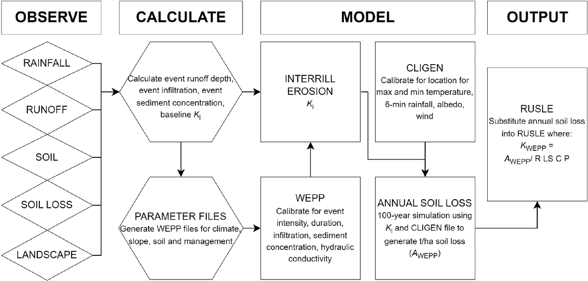
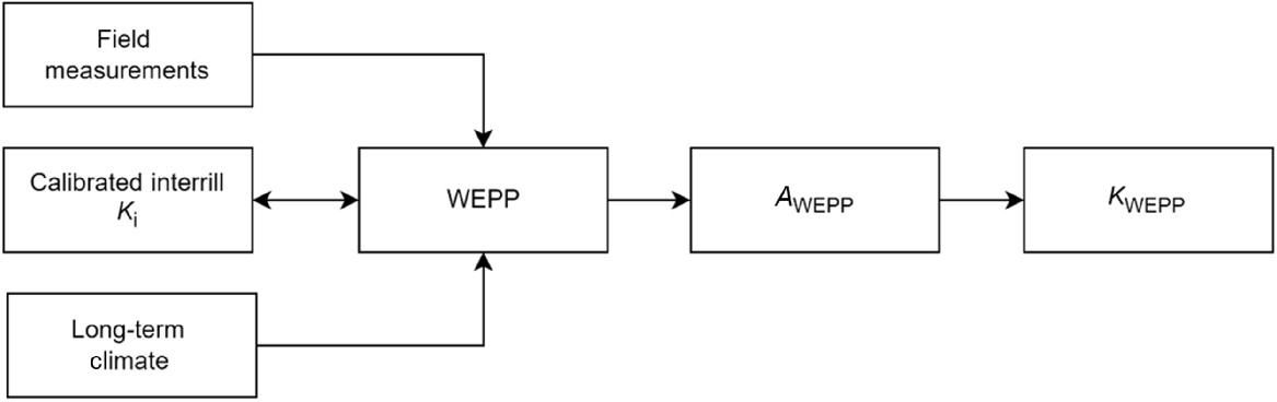
This is essentially a two-part process where WEPP was calibrated based on field measurements and used to calculate event hydrological and sediment data, which were input into WEPP to estimate erodibility parameters (Ki). The calibrated parameter values, along with site-derived long-term climate data, were then used to run a simulated climate scenario for a 100-year period to generate a long-term mean annual soil loss resulting in AWEPP. The AWEPP was then used to compute KWEPP using RUSLE (Fig. 2), where AWEPP was substituted for A in Eqn 4.
Site description
Data were collected from two beef cattle grazing properties within the semi-arid Fitzroy Basin: (1) the Brigalow Catchment Study and surrounds in 2017; and (2) Belmont Research Station in 2021 (Fig. 3).
Relative location of the Fitzroy Basin in the Great Barrier Reef catchments, Queensland, Australia (left), and study locations within the Fitzroy Basin (right).
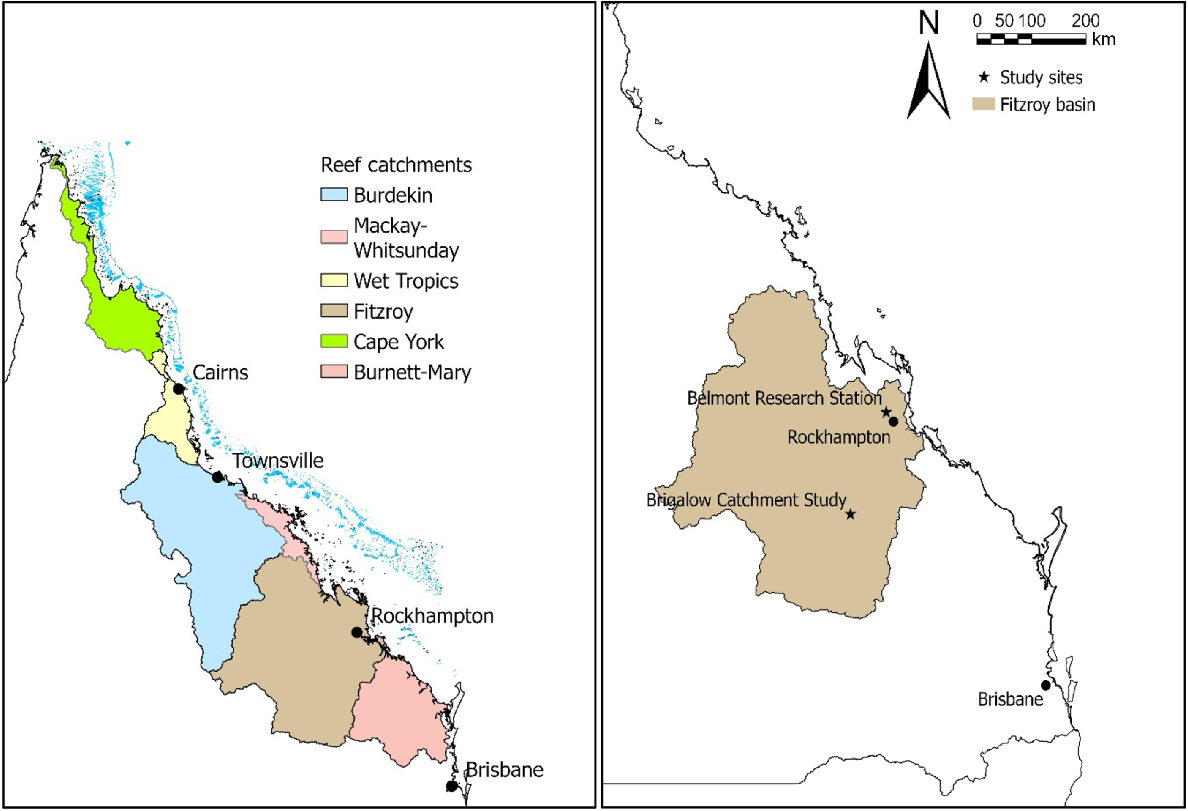
The Brigalow Catchment Study is located near Theodore in central Queensland (24.81°S, 149.80°E, GDA 94) and was described in detail in Cowie et al. (2007). It is located in the Dawson River catchment of the Fitzroy Basin, and the climate is semi-arid to subtropical with a mean annual rainfall of 650 mm. Average maximum monthly temperature in summer is 33°C (December–February) and average minimum temperature in winter of 6.5°C (June–August). Four sites were investigated in this location: two Brown Sodosols and two Black Vertosols. Sites with similar soil types showed enough soil texture variation to be considered separately as Vertosol1 and Vertosol2, and Sodosol1 and Sodosol2. These soil types are representative of 56% of the Fitzroy Basin with the land use of grazing: Vertosols (28%) and Sodosols (28%) (Roots 2016; Elledge and Thornton 2017). The two Sodosols in this study have a low average exchangeable sodium percentage (ESP) in the 0–0.1 m depth of 0.4% for Sodosol1 and 4.5% for Sodosol2. Vertosol1 showed ESP at the depth of 0–0.1 m was 6.8%, indicating marginal sodicity (Hazelton and Murphy 2007).
Belmont Research Station is located approximately 37 km north of Rockhampton adjacent to the Fitzroy River in the Fitzroy catchment of the Fitzroy Basin (23.23°S, 150.39°E GDA 94) and was described in detail in Coventry and Murtha (1976). The station is located close to the Tropic of Capricorn, and the climate is sub-tropical with a mean annual rainfall of 800 mm. Average maximum monthly temperature in summer is 32°C (December–February), and average minimum monthly temperature in winter is 9°C (June–August). Two sites and soil types were investigated in this location including a Leptic Tenosol and a Black Dermosol. These soils are collectively representative of 14% of the Fitzroy Basin under grazing: Dermosols (11%) and Tenosols (3%) (Roots 2016).
Treatments
All soils were studied in situ to preserve soil consolidation and organic bonds. The plot surface was prepared as an artificially scalded surface to represent consolidated bare ground by mechanically removing the surface organic A1 horizon to expose the hard-set layer beneath and was left to weather and reconsolidate for up to three months. Use of artificial scalds in place of natural scalds was validated in Loch (2015a) and Loch (2017).
The Vertosol and Sodosol soils had an additional natural scald treatment as well as an artificial scald. This treatment identified bare surfaces which had been weathered in situ for at least a year, eroding the remnant A surface horizon to a hard-set layer.
Rainfall simulation, runoff generation, and water quality sampling
Plots were bunded by inserting flat galvanised panels approximately 0.2 m high into the ground to a depth of at least 0.05 m. The plots sizes on the Brigalow Catchment Study were 2.0 m × 1.5 m (3 m2) and those on Belmont Research Station were 2.0 m long by 1.4 m wide (2.8 m2). All plots were on slope gradients less than 5%. A triangular galvanised flume narrowing into a collection pipe was placed downslope to collect runoff water. The difference in plot sizes was due to the width of the flume available at the time of the experiment. Potable water, or rainwater, with low electrical conductivity (<200 mS m−1) was applied using the rainfall simulator described in Loch et al. (2001) at a target intensity of 80 mm h−1 with VeeJet 80100 nozzles. The target intensity was selected to meet a one in 20 year rainfall event as determined by the Bureau of Meteorology Average Recurrence Interval data (Bureau of Meteorology 2022). Runoff was collected in 1-L sample bottles at the commencement of steady state runoff, with water quality samples taken every 3–5 min for 20–30 min. Each runoff sample was timed during collection and weighed after the event to calculate a runoff rate (mm h−1). Water quality samples were analysed at the Department of Environment, Tourism, Science and Innovation Chemistry Centre for total solids and volatile solids (method 2540B) and total suspended solids (method 2540D). Water analysis methods were based on APHA AWWA (2012). Each site was visited once with three rainfall simulation repetitions conducted on each soil type and treatment. A comparison of the observed hydrograph and sediment output per plot and treatment was conducted to validate each plot.
Soil sampling
Surface soil samples (0–0.1 m) were collected pre- and post-rainfall simulation events to determine soil moisture conditions. Soil cores were analysed for air dried moisture content, cation exchange capacity, total organic carbon, bulk density, and particle size fractions of clay, silt, and sand using the methods of Rayment and Lyons (2011). Percent of undispersed particles less than 0.125 mm in the rainfall wet soil surface (P125) was determined according to Loch and Rosewell (1992) (Table 1).
| Soil | Plot area (m2) | Slope (%) | Clay (<0.002 mm) (%) | Silt (0.02–0.002 mm) (%) | Fine sand (0.2–0.02 mm) (%) | Coarse sand (>0.2 mm) (%) | P125 (<0.125 mm) (%) | Estimated wet density (Mg m−3) | Organic carbon (%) | Cation exchange capacity (cmolc kg−1) | Bulk density (g cm−3) | |
|---|---|---|---|---|---|---|---|---|---|---|---|---|
| Dermosol | 2.8 | 3.5 | 30.1 | 24.4 | 22.1 | 25.0 | 63.7 | 1.68 | 1.52 | 18 | 1.31 | |
| Sodosol1 | 3.0 | 2.8 | 10.7 | 4.2 | 39.9 | 49.4 | 32.9 | 2.31 | 0.96 | 13 | 1.58 | |
| Sodosol2 | 3.0 | 3.3 | 20.9 | 7.4 | 39.2 | 36.3 | 52.6 | 2.02 | 0.73 | 10 | 1.65 | |
| Tenosol | 2.8 | 5.0 | 19.8 | 31.2 | 23.6 | 30.1 | 64.8 | 1.70 | 1.25 | 13 | 1.42 | |
| Vertosol1 | 3.0 | 2.2 | 34.8 | 10.7 | 35.6 | 27.7 | 49.1 | 1.82 | 0.85 | 25 | 1.54 | |
| Vertosol2 | 3.0 | 2.3 | 26.1 | 7.5 | 37.8 | 29.8 | 48.2 | 2.00 | 1.53 | 18 | 1.62 |
P125 is the percentage of undispersed soil particles <0.125 mm in the soil surface after rainfall wetting (Loch and Rosewell 1992).
Soil erosion modelling: WEPP
The WEPP can be used for multiple-year, long-term simulations as well as single event simulations. For this study, WEPP v2012.8 was run for each experimental plot using the single storm option and plot-specific input files accounting for soil properties, slope geometry (length and slope), ground cover, and rainfall intensity. Soil hydraulic conductivity (Ke) was calibrated in the soil file until the WEPP single storm infiltration rate equalled the observed steady state infiltration rate per plot. The Ke was averaged per soil type and treatment. Steady state was defined as the period when the hydrograph and sediment concentration are constant over time, as distinct from noticeable fluctuations at the beginning of the runoff event. Interrill erodibility in the individual WEPP soil files was adjusted to match modelled sediment loss per unit width (kg m−1) against observations. The observed soil loss was related to observed steady state concentration (g L−1) and converted to kg m−1 via:
where E is the soil loss per unit width (kg m−1), c is the steady state concentration (g L−1), L is slope length (m), and Q is total runoff depth (mm).
Long-term climate data for Belmont Research Station covered a period of 45 years based on Bureau of Meteorology (data from the Rockhampton station. Climate data for the Brigalow Catchment Study were collected onsite, providing a 43-year dataset. These climate data were used to generate the 100-year weather simulation using CLIGEN v5.3.
Soil erosion modelling: RUSLE
The RUSLE equation (Renard et al. 1997) follows:
where A is annual soil loss (t ha−1 year−1); R is the annual rainfall erosivity (MJ mm ha−1 h−1 year−1); K is soil erodibility (t h MJ−1 mm−1); L and S are the slope length and slope steepness factors, collectively referred to as the LS factor; C is the crop cover and management factor; and P is practice factor which includes contouring, terracing, and other conservation practices. The LS, C, and P are unitless, describing the deviation from a USLE unit plot. The USLE unit plot is defined as a length of 22.1 m with a 9% slope, tilled up and down the slope, and retained as bare fallow conditions. Units here are expressed as SI units converted from the original imperial measure by Foster et al. (1981).
For erodibility, the equation for the USLE nomograph K (Knom) in SI units (t h MJ−1 mm−1) for soils with less than 70% silt used by Rosewell and Edwards (1988) in Australian studies follows:
where M = (percent silt + percent very fine sand) (100 − percent clay), OM is organic matter (%), SS is the soil structure code, and PP is the profile permeability class. The particle size class defined for silt plus very fine sand is 0.002–0.1 mm and for clay is the less than 0.002 mm fraction.
The Loch et al. (1998) nomograph modification (Km) adjusts the definition of M, where M is replaced by 100(P125), P125 is particle size distribution less than 0.125 mm, and by using estimated or measured wet sediment density from Loch and Rosewell (1992). Eqn 3 and the Km modification are used in the GBR Dynamic SedNet and were therefore selected for this study.
In the RUSLE, the ratio of the average soil loss (A) per unit of rainfall erosivity (R) for a unit plot under continuous fallow is represented as K = A/R. In this experiment, LS and C were used to represent a low rill/interrill relationship on a bare plot, and the resulting K-factor follows:
The soil loss A was estimated from WEPP by running 100-year simulations based on the plot-calibrated effective hydraulic conductivity (mm h−1) and interrill erodibility (kg s m−4) per soil type. The R was obtained from table 2 in Yu (1998) using Station 39083 for Belmont Research Station, and Station 39090 for the Brigalow Catchment Study. A 100-year simulation was run in WEPP to model the annual average soil loss output (AWEPP) at a slope length of 22 m as reflective of the initial USLE plot at a 9% gradient. The C-factor parameters were adapted from the cover factor equation in Rosewell (1993) where 0.45 is for bare ground (Silburn 2011). The P-factor was set to 1 as it was not applicable here.
Data analysis
RStudio version 4.2.2 was used to analyse and generate graphics of the data using base R, elements of tidyverse including dplyr (Wickham et al. 2023) and ggplot (Wickham 2016) packages. Other packages used to explore and analyse the data include broom (Robinson et al. 2023), multcomp (Hothorn et al. 2023), and car (Fox and Weisberg 2019). Post hoc Bonferroni adjusted multiple comparison analysis was used to identify group differences. Results in Tables 2 and 3 are presented with alphabetical letters where groups not sharing the same letter differ at the 5% level. Performance measures used to compare WEPP models with observations include R2, PBIAS, and NSE (Samantaray et al. 2024, 2025). They are defined below, where OBS is observed data, is the mean, and SIM is the WEPP simulated results. The R2 is based on the formula used in tidyverse where SS is sum of squares for residuals (res) and totals (tot).
Results
Measured data for the rainfall simulation plots
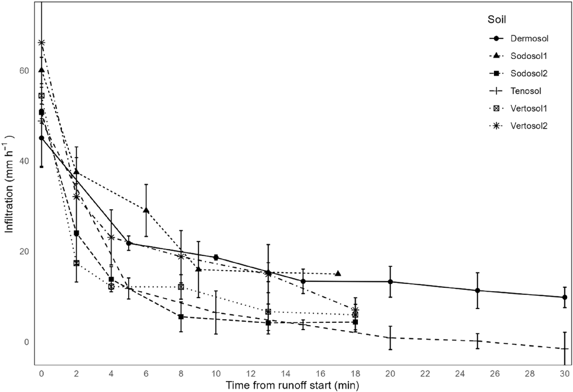
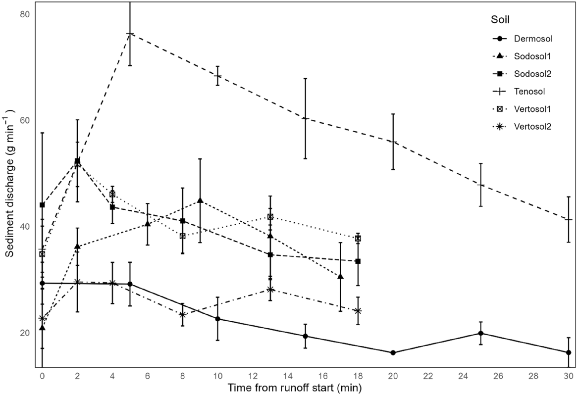
There were no significant differences for any parameter between natural and artificial scalds on Vertosols and Sodosols (P > 0.7). Based on this result, hydrograph properties for the natural and artificial scalds on these two soil types were combined (Table 2). Minimal to no rilling was observed in the 2-m plots. Runoff started 1.5–4.3 min after the commencement of simulated rainfall, and soils with a higher clay and silt content began runoff earlier. A similar trend was noted for steady state infiltration (mm h−1) where coarser textured soils maintained a higher infiltration rate. Sediment loss peaked early in the runoff events (0–5 min) and gradually declined with time for most plots. Most plots had an observable steady state, with soil loss remaining relatively constant across most times steps except for the Tenosol, which consistently declined for each time step, as did Sodosol2 to a lesser degree. Steady state observations are summarised for infiltration (mm h−1), sediment concentration (g L−1), sediment generation (g min−1), and runoff rate (mm h−1) in Table 2.
| Soil | n plots | Slope (%) | Time to runoff (min) | Rainfall intensity (mm h−1) | Rainfall duration (min) | Runoff rate (mm h−1) | Runoff depth (mm) | Infiltration rate (mm h−1) | Sediment concentration (g L−1) | Sediment discharge (g min−1) | |
|---|---|---|---|---|---|---|---|---|---|---|---|
| Dermosol | 2 | 3.5 | 1.5c | 84 | 33 | 72.3(0.3)b | 44.2(0.4)d | 11.5(1.2)ab | 5.4(0.2)b | 18.0(0.7)b | |
| Sodosol1 | 2 | 2.8 | 4.0a | 77 | 20 | 54.0(2.4)c | 31.8(0.3)c | 16.2(0.9)a | 13.1(1.3)a | 36.5(2.4)ab | |
| Sodosol2 | 6 | 3.3 | 2.0c | 88 | 20 | 83.4(0.6)a | 26.3(0.4)b | 5.1(0.3)b | 8.6(0.4)ab | 36.4(1.9)ab | |
| Tenosol | 3 | 5.0 | 1.7c | 82 | 33 | 81.1(0.9)ab | 43.3(0.4)d | 6.4(0.6)b | 12.8(0.2)a | 51.4(2.0)a | |
| Vertosol1 | 3 | 2.2 | 2.7b | 91 | 20 | 79.3(0.7)ab | 32.4(0.2)c | 8.5(0.8)ab | 10.1(0.1)ab | 40.9(0.2)ab | |
| Vertosol2 | 6 | 2.3 | 3.7a | 83 | 20 | 75.1(0.5)b | 28.4(0.3)a | 8.2(0.4)b | 7.4(0.2)b | 25.7(0.9)b |
Means followed by the same letter within columns are not statistically different. Standard errors are given in parentheses.
The Dermosol, while higher in clay content (30%) and with a low estimated wet density (1.68 Mg m−3), had a high steady state infiltration rate, exceeded only by the sandy loam of the Sodosol1. The Dermosol and Tenosol runoff depths were the highest at 44 and 43 mm, respectively. Runoff depth results are caveated by the differences in rainfall duration, with most sites receiving 20 min of rain except for the Dermosol and Tenosol with 33 min. All plots receiving ~20 min of rain had runoff depths of 26–32 mm. Runoff initiated earliest at 1.5 min on the Dermosol. The Dermosol had the lowest sediment generation (18.0 g min−1) and concentration (5.4 g L−1) of all soils investigated. The runoff rate from all Dermosol plots averaged 72 mm h−1 with an average rainfall intensity of 84 mm h−1.
The Sodosol1 was a loamy sand textured soil with a low clay and silt content (9.9% and 3.4%, respectively), and time to runoff from rain initiation was the slowest at 4.0 min. Infiltration was the highest (16 mm h−1) as was sediment concentration (13.1 g L−1). Sodosol1 had the lowest runoff rate (54 mm h−1). In contrast, Sodosol2, which had a higher clay and silt content (20.9% and 7.4%, respectively), had the lowest infiltration rate (5.1 mm h−1), the highest runoff rate (83.4 mm h−1), and the lowest runoff depth for plots receiving 20 min of rain (26.3 mm). The Tenosol had the highest sediment rate (51.4 g min−1) and second highest sediment concentration (12.8 g L−1).
The Vertosol1 showed differences to Vertosol2, with the higher mean rainfall intensity (91 mm h−1) resulting in a higher runoff rate, depth, sediment concentration, and sediment rate than Vertosol2. Soil particle size fractions were similar between the two Vertosols; however, Vertosol2 had higher organic carbon (1.53%) than Vertosol1 (0.85%). Sediment concentration and sediment generation for Vertosol2 were low.
All steady state factors of infiltration (mm h−1), runoff rate (mm h−1), sediment concentration (g L−1), and sediment generation rate (g min−1) significantly differed between soil types (P < 0.002). Significant differences were observed between most soil types for runoff depth (mm), primarily influenced by differing rainfall durations and therefore the P-value is not shown here.
Infiltration rates decreased as time increased (Fig. 4), whereas runoff rates increased (Fig. 5). For Sodosol1 and to a limited degree Vertosol2, sediment transport increased initially before decreasing as time passed (Fig. 6). Steady state sediment generation was achieved for most soils, with the Tenosol and Sodosol1 the exceptions. For the Tenosol, and to a lesser degree Sodosol1, sediment generation was still declining at the end of the rainfall event (Fig. 6).

WEPP modelling outputs
Each plot repetition per soil and scald treatment were validated using comparisons of the observed plot hydrograph and sediment output, then combined by treatment and soil type. Artificial scalds were the only treatment observed on the Dermosol and Tenosol. Data modelled in WEPP for infiltration rate (Ke, mm h−1), mean interrill erodibility (Ki, ×106 kg s m−4), annual soil loss (t ha−1), and the cover factor are shown in Table 3 alongside modelled KWEPP (erodibility) parameters (t h MJ−1 mm−1). Initial KWEPP was the result of K = A/R prior to applying Eqn 4.
| Soil | n plots | RUSLE R-factor (Yu 1998) | WEPP mean infiltration (Ke) (mm h−1) | Calculated Ki using Elliot et al. (1989) (kg s m−4 × 10⁶) | WEPP mean interrill erosion rate (Ki) (kg s m−4 × 10⁶) | WEPP annual soil loss (t ha−1) | C-factor | KWEPP initial (t h MJ−1 mm−1) | Average Knom (t h MJ−1 mm−1) | Average Km (t h MJ−1 mm−1) | Average KWEPP (t h MJ−1 mm−1) | |
|---|---|---|---|---|---|---|---|---|---|---|---|---|
| Dermosol | 2 | 3152 | 2.3b | 0.57c | 0.97b | 20.6 | 0.39 | 0.007 | 0.032 | 0.045 | 0.017 | |
| Sodosol1 | 2 | 2683 | 20.0a | 1.61ab | 1.57ab | 31.6 | 0.45 | 0.012 | 0.029 | 0.032 | 0.026 | |
| Sodosol2 | 6 | 2683 | 2.4b | 1.12bc | 1.12b | 46.4 | 0.45 | 0.017 | 0.034 | 0.036 | 0.038 | |
| Tenosol | 3 | 3152 | 0.7b | 1.90a | 2.26a | 39.4 | 0.45 | 0.013 | 0.040 | 0.048 | 0.028 | |
| Vertosol1 | 3 | 2683 | 5.9b | 1.31abc | 1.06b | 21.4 | 0.45 | 0.008 | 0.035 | 0.042 | 0.018 | |
| Vertosol2 | 6 | 2683 | 5.3b | 0.97bc | 0.96b | 21.0 | 0.45 | 0.008 | 0.033 | 0.034 | 0.017 |
Means followed by the same letter within columns are not statistically different.
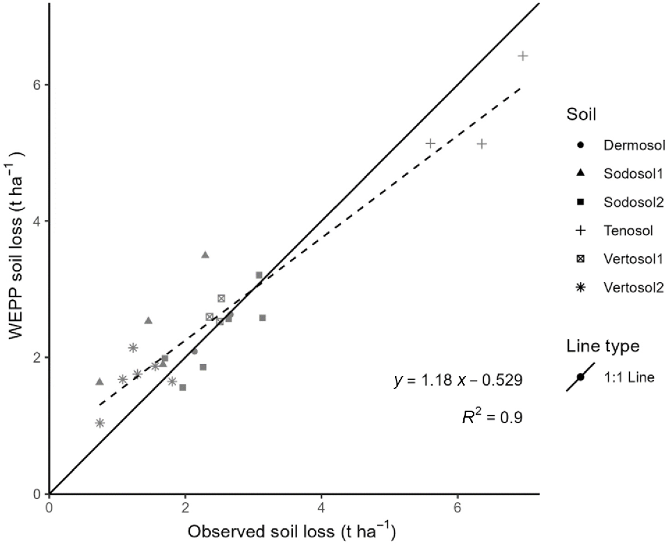
Total observed soil loss (t ha−1) from each simulated rainfall event was compared to the WEPP modelled soil loss on a plot-by-plot basis to assess WEPP outputs (Fig. 7). The model fit (R2 = 0.9, PBIAS = 1.9%, NSE = 0.87) indicates good confidence that the plot calibrations are acceptable.
Comparison of observed plot-scale soil loss for each simulated rainfall event against WEPP-modelled soil loss per plot (R2 = 0.9, PBIAS = 1.9%, NSE = 0.87, n = 24).
The WEPP mean infiltration (Ke) was calibrated per plot then averaged across each repetition per scald treatment and soil type. Where a plot was not valid, it was dropped from analysis. Hydrological anomalies observed for Vertosol1 reduced a potential six plots to three, and on Sodosol1, six plots were reduced to two. The Dermosol included two plots of a potential three. Modelled Ke appeared to follow the same observed steady state infiltration rate trends as field observations, where the sandier textured Sodosol1 showed considerably higher Ke (20.0 mm h−1). The Tenosol had the lowest Ke of 0.7 mm h−1. The Ke significantly differed between soil types (P < 0.001) (Table 3).
Interrill erosion (Ki) parameters significantly differed between soil types (P < 0.001). Calculated Ki based on Elliot et al. (1989) was tested against modelled WEPP Ki and showed good agreement for most soils and both approaches, with derived Ki not significantly different (P = 0.9). The highest Ki value was for the Tenosol of 2.26 × 10⁶ kg s m−4 and the lowest was 0.96 × 10⁶ kg s m−4 for Vertosol2.
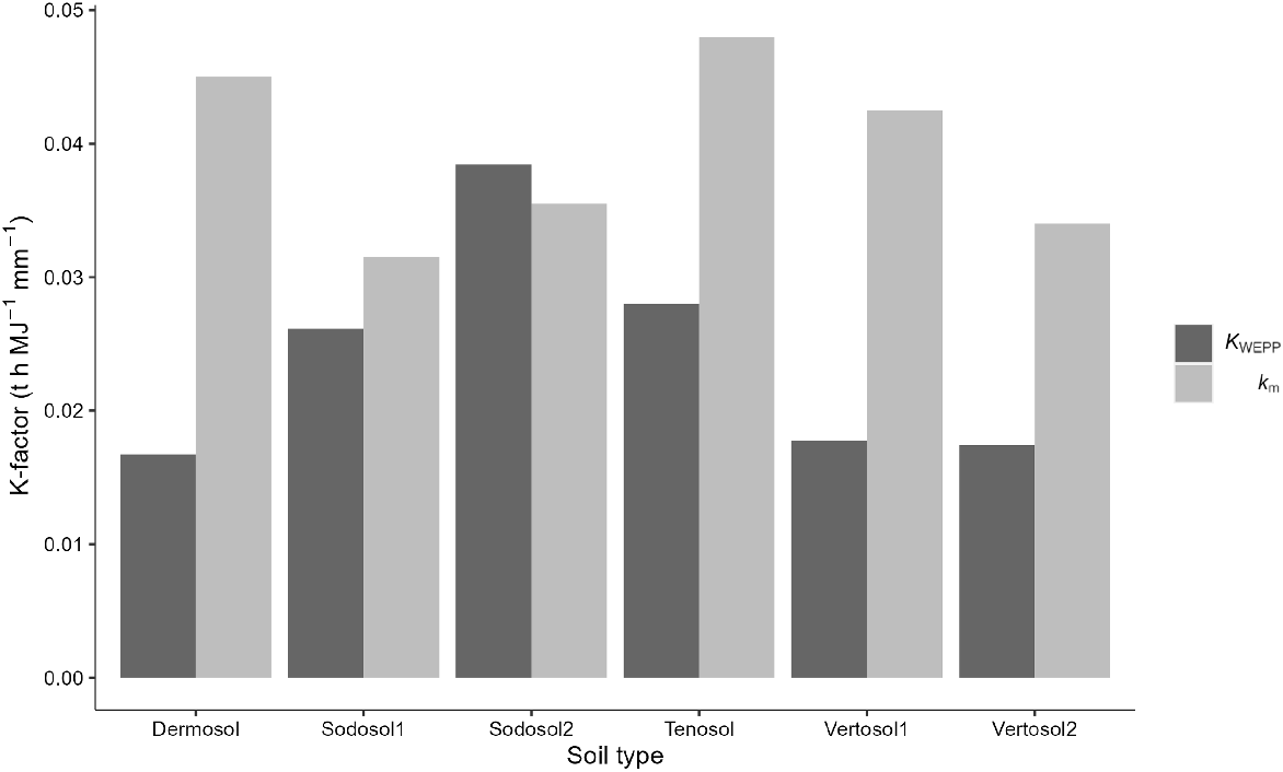
The Km (modified nomograph) across all soils ranged between 0.032 and 0.048 t h MJ−1 mm−1, indicating moderate erodibility for each soil studied. For Knom, the range was 0.034–0.040, also indicating moderate erodibility for all soils. When using AWEPP to substitute into RUSLE, the resultant KWEPP range for most soils was 0.017–0.028, indicating low erodibility class, with Sodosol2 the only moderately erodible soil (0.038), which was also the highest K-factor in this study for KWEPP. For Sodosol2, Km is within 8% of the modelled KWEPP. The Dermosol and Vertosol1 showed the lowest KWEPP erodibility (0.017, low erodibility), noting the Dermosol had enough rock cover on the bare surface to reduce the C-factor to 0.39.
The KWEPP was up to 63% lower than Km for all soils, except Sodosol2 where it was 8% higher (Fig. 8). Vertosol1 and Vertosol2 were 49% and 58% lower, respectively, when comparing KWEPP to Km. Both nomograph-calculated K-factors (Knom and Km) indicated moderate to high erodibility for Vertosols (range 0.033–0.042). Sodosol1 was 17% lower for KWEPP than Km. The Tenosol was 42% lower for KWEPP and the Dermosol 63% lower for KWEPP.
Discussion
WEPP/RUSLE integration
Limited Australian studies have investigated estimating soil erodibility using WEPP as a substitute for RUSLE, with the exception of developmental work undertaken between 2015 and 2017 as part of the Paddock to Reef Integrated Monitoring and Modelling Program reported in Loch (2017). In Loch (2017), data observed for the Brigalow Catchment Study were modelled using shorter slope length than this study (11 m by 4%) and an extended version of WEPP not publicly available. Loch (2017) used a modified version of WEPP v2012.8, which allows up to 10 different soil size classes as opposed to the three classes used in the publicly available WEPP v2012.8 version, introducing a variability this study cannot account for. No specific methodology or WEPP soil, management, and climate files used to develop K-factors in Loch (2017) are available and were subsequently independently developed for this study.
Internationally, there have been several studies comparing erodibility from the RUSLE and the WEPP. Nearing and Nicks (1998) compared erodibility of 45 soils in the USA and noted that direct comparison between the RUSLE and WEPP erodibilities is complicated by the inclusion of three erodibility-related parameters within WEPP (interrill, rill, and critical shear stress); however, there was no statistical bias between the two model outputs.
Laboratory experiments by Deviren Saygin et al. (2018) investigated the combination of WEPP and RUSLE to estimate the USLE erodibility factor. Deviren Saygin et al. (2018) used laboratory-based rainfall simulation plots to separately calculate interrill and rill parameters to input into WEPP to output an annual soil loss over a 100-year simulation to calculate K. Modelled K in their study was significantly lower than the empirical RUSLE equations for K. The approach by Deviren Saygin et al. (2018) differed to this study by applying a monthly tillage in the WEPP model, where this study considers a permanent consolidated surface as found on grazed hillslopes. That study also used soil transferred to laboratory plots to apply simulated rain, which may not represent the consolidation and organic bonds of in situ soil.
Interrill erosion
As ascertained in Yu and Rosewell (2001), WEPP is a complex process-based model comprising a significant number of initial parameters and sub-routines. Every effort was made to set initial parameters as accurately as possible, based on observed site data. All erosion observed was interrill erosion, as expected for plots with short lengths and low slopes. While this study attempted to isolate interrill erosion specifically as the driver for soil loss, the WEPP model still considers rill formation when scaling the plot data to a 22 m slope length, contributing some rilling to the sediment transport output.
Interrill erosion processes are dominated by raindrop impact and subsequent sediment transport of overland flow (Kinnell 2005; Zhang et al. 2020). When raindrop detachment is greater than the transport capacity of overland flow, the system is transport-limited; if flow is greater than the ability of raindrops to detach soil particles, the system is detachment-limited (Zhang et al. 2020). Both transport- and detachment-limited processes were observed in this study, where initial sediment loss peaked early where raindrop-impact detached soil, declining with time as entrainable sediment supply reduced, and the ability for raindrop impact to disperse particles was less effective as depth of flow increased. In this study, low slopes inhibited flow transport and are representative of the low gradient of grazed lands in the Fitzroy Basin.
Assessing sediment output using WEPP has been tested in several studies. In Australia, Yu and Rosewell (2001) validated soil loss prediction on bare fallow plots, providing confidence in the substitution of A in the RUSLE for soil loss prediction on similarly prepared plots to this study. The WEPP has been successfully applied in various USA conditions to predict sediment yield (Ghidey and Alberts 1996; Ahmadi et al. 2011). Accurately representing the hydrology and climate variables assists in better predictability of soil loss (Laflen et al. 1994), and with known parameters of the rainfall event applied to the plot, measured hydrology, and an appropriately-generated CLIGEN file, the calibration to simulate soil loss was applied with the best available data.
Modelled K-factor
In soils with similar totals of clay and silt (approximately 50% combined total for the Dermosol, Tenosol, and Vertosol1), observed sediment loss, infiltration, and sediment transport varied significantly. These differences may be influenced by variations in the soil properties of cation exchange capacity and organic matter as captured in the nomograph; however, the variation between the nomograph equations (Km and Knom) and the modelled KWEPP are worthy of discussion. The modified nomograph (Km), limited to soil properties, indicates that all soils are moderately erodible, with the Tenosol, Dermosol, and Vertosol1 at the high end of the moderately erodible scale. The Knom follows a similar trend; however, KWEPP disagrees with Km and Knom.
As an example, the Tenosol had the highest Km (0.048) and Knom (0.040) but was in the low erodibility class for KWEPP (0.028), despite having the highest sediment discharge rate and interrill erosion parameter. Literature shows that Tenosols can vary from low to high erodibility. Silburn (2011) provides a measured K-factor for an Orthic Tenosol of 0.050 in central Queensland’s Nogoa sub-catchment of the Fitzroy Basin, and for a Tenosol in Victoria’s LaTrobe catchment, Vigiak et al. (2011) provides an estimate of 0.015; however, the Tenosol in Victoria had very low clay (1%) and very high organic matter (12%). The Tenosol in Silburn (2011) had 12% clay and low organic matter of 0.6%. The KWEPP of 0.028 modelled here is a likely representation of in situ, undisturbed soil and seems reasonable for a Tenosol, as is Km of 0.048.
Vertosol1 and Vertosol2 sites were located within the conservatively grazed catchment of the Brigalow Catchment Study. This catchment has a long-term observed soil loss of 0.26 t ha−1 year−1 for the years 1984–2010 (Thornton and Elledge 2021). Substituting KWEPP (0.018) into the RUSLE equation as K, and appropriate parameters for the catchment (LS = 0.37; R = 2683; C = 0.013), the soil loss estimate was 0.23 t ha−1 year−1. Using the average Km for Vertosol1 and Vertosol2 (0.038), the predicted soil loss output was 0.49 t ha−1 year−1; double the observed data. A K-factor developed by Loch (2017) with a similar WEPP and RUSLE integration based on the same observed dataset (K = 0.023) when substituted into RUSLE, also provided a reasonable estimate for this same catchment (0.30 t ha−1 year−1) compared to the long-term observed soil loss. An analysis of the Modified USLE (MUSLE) by Tiwari et al. (2021) estimated this conservatively grazed catchment had a K-factor of 0.059 which was significantly higher than the WEPP-derived K estimates provided here.
Vertosols are prevalent in the Fitzroy Basin (28% of the grazed land use). Vertosols studied by Freebairn et al. (1996) at the Darling Downs, Queensland, indicate that Vertosols are highly erodible, specifically on cropping systems. The soils in that study had in excess of 50% clay unlike this study. Sediment loss data from the Freebairn et al. (1989) study were evaluated against the USLE, and it was reported that deriving erodibility from the nomograph equation was determined to be unreliable for high clay soils (Freebairn et al. 1989). Measured erodibility from the cropping trial by Freebairn et al. (1989) was used as a point of validation for modelling erodibility using WEPP and RUSLE by Loch (2015b), which showed reasonable agreement, indicating the use of WEPP to derive an annual soil loss average to substitute into RUSLE is feasible.
Aggregate stability is an indicator of susceptibility to erosion (Barthès and Roose 2002; Ben-Hur and Lado 2008), particularly the interaction of clay particles (Lado and Ben-Hur 2004). Vertosols are characterised by high clay content (Isbell and National Committee on Soil and Terrain 2021) and Murphy et al. (2013) makes the point that when wet, Vertosols are highly erodible. At the time of the rainfall simulation study on the Vertosols, the soil moisture prior to applying rain was low (~4%). This study showed variation of sediment discharge between the Vertosols modelled (40.9 and 25.7 g min−1). This may be explained by variations in soil organic carbon (SOC) and clay fractions, with Vertosol1 exhibiting lower SOC (0.85%) and higher clay content (34.8%) than Vertosol2 (1.53% and 26%, respectively). Despite these differences, and variations in cation exchange capacity and soil texture, the Ki modelled for the Vertosols was similar (1.06 × 10⁶ and 0.96 × 10⁶ kg s m−4) and, as a result, so was the KWEPP simulated under the same climactic conditions (KWEPP 0.018 and 0.017).
Using the Sodosol1 dataset, Loch (2017) modelled a 100-year WEPP simulation with a slope length of 11 m by 4% slope with different RUSLE C-factors (0.07 and 0.43) and calculated an average KWEPP of 0.038, which was higher than the modelled output here (KWEPP 0.026) by 32%. For Sodosol2, Loch (2017) derived an average of 0.020 at a LS of 11 m by 4% (C-factor, 0.43). Using a C-factor of 0.45 and a 22 m by 9% LS in this study, Sodosol2KWEPP was 0.038, which presents a significant difference. On a larger spatial scale (74 m2), Silburn (2011) calculated a K-factor value of 0.042 for a sandy clay loam, a Brown Sodosol, near Springvale, Queensland, over seven years of observation. This is reasonably comparative to Sodosol2 but 38% higher than Sodosol1. The soil texture properties of Sodosol1 were more similar to the Sodosol studied by Silburn (2011) than Sodosol2. Local variation is therefore relevant and site-specific K-factors would be useful.
One of the few Australian studies where K-factor was measured were on cultivated modified USLE plots (41 m × 2.44 m, 10% slope, 107 m2) was in Wagga Wagga, New South Wales, where five soils were observed over 4–8 years by Rosewell (1992). That study highlighted the influence of rainfall erosivity variations from year to year on a sandy clay loam (Northcote Principal Profile Form: Dr2.32) similar to Sodosol2, which generated K-factors of 0.003–0.121. This substantial variability indicates that rainfall erosivity variations over time are relevant, highlighting that long periods of in situ measurement of soil loss are generally advisable to determine the K-factor. In this study, long-term climate variables were captured in the WEPP modelling using CLIGEN, which were based on a long-term rainfall dataset. The variability of the Sodosols across the above studies makes it difficult to assess an appropriate K-factor; however, considering the sodic influence within the Sodosol soil group, erodibility values have the potential to be significant.
This same study by Rosewell (1992) investigated a possible medium clay Dermosol at Inverell, New South Wales (Northcote Principal Profile Form: Uf6.21) on a bare fallow USLE plot 41 m in length at 10% slope, reporting an average K-factor of 0.017. Annual variations observed there were 0.007–0.061. At the same site, a heavy clay Dermosol (Northcote Principal Profile Form: Uf6.21) had an average K of 0.045 (annual variation 0.018–0.070). The Dermosol in this study showed more soil texture similarities to the heavy clay soil at Inverell. A black Dermosol was investigated by Silburn and Bosomworth (2023) in a cropping scenario, and they determined Ki of 3.9 × 10⁶ kg s m−4, which was significantly higher than Ki estimated in this study (0.59 × 10⁶ kg s m−4). While both Dermosols had similar clay and silt contents, the loose, unconsolidated condition of the cropping Dermosol resulted in high soil loss under laboratory-simulated rainfall conditions (29.3 t ha−1) compared to in situ plots in this study where the consolidated Dermosol soil averaged a soil loss of 2.4 t ha−1 (Fig. 7). Consolidation may explain the difference in Ki, as well as the cropping Dermosol having considerably higher fine sand content (45%) than the grazing Dermosol of this study (22%). Considering that Dermosols can have high clay or loamy textures, the response to detachment and transport of sediment will be soil and site specific. The K-factor modelled in this study of 0.017 is therefore reasonable and representative of a cohesive surface.
Particle size
The study data suggest cohesiveness, consolidation, and aggregation present in the soil surface influence detachment compared to an erodibility nomograph equation which expects some surface disturbance (e.g. cultivation). Soil aggregate strength, specifically consolidation of in situ soils, influences particle detachment and erodibility, and is integral in erosion resistance (Bryan 2000; Ben-Hur and Lado 2008; Thomaz and Fidalski 2020; Xia et al. 2022; Liu et al. 2023). While particle size is an influential factor, as mentioned by several authors, a variety of other factors increase or decrease resistance to detachment, surface sealing, and entrainment (Alberts et al. 1987; Ben-Hur and Agassi 1997; Ben-Hur and Wakindiki 2004). This was observed here where differing soil property combinations modelled different AWEPP and KWEPP values. The Dermosol and Tenosol had high silt percentages of 24% and 31%, respectively, compared to the other soils; however, these soils exhibited vastly different Ki and KWEPP values. The Dermosol had rock content on the surface and within the soil profile, which may have assisted with infiltration pathways despite a high runoff depth, and thereby inhibited sediment export. Sodosol1 had low clay and silt (~15% combined) and a higher presence of sand fractions, resulting in a high Ki, whereas Sodosol2 had a lower Ki yet had the highest KWEPP of all soils studied. Sodosol2 had the lowest organic carbon percentage (0.73%), generally an indicator of weaker aggregate strength; however, this alone does not explain the high KWEPP, as Vertosol2 and Sodosol1 had organic carbon less than 1% and modelled low KWEPP erodibility.
KWEPP implications
With the exception of Sodosol2, KWEPP was consistently lower than Km and Knom. This suggests that hillslope RUSLE modelling in Dynamic SedNet, which currently implements Km, may be overestimating hillslope sediment loss. This has been highlighted in this study where observed and modelled K-factors showed a substantially lower KWEPP than both erodibility nomograph equations. The nomograph, and indeed the RUSLE, assume a disturbed surface soil not always present on grazed hillslopes when not considering animal traffic itself. Reichert et al. (2001) indicates that increased soil aggregation, consolidation, and surface residue reduce erosion. These conditions are analogous to a grazed hillslope as studied here, so a similar response would be expected.
For the soils considered in this study, which together comprise approximately 70% of the area grazed in the Fitzroy catchment, hillslope erosion could be overestimated, specifically on bare, consolidated ground. With increased ground cover on consolidated soils, the expected soil loss response from hillslope grazing would decrease.
In this study, a storm event was set at one intensity to develop soil loss outputs, then an average long-term erosivity (R) was applied to determine KWEPP. Undertaking further research over a range of storm event intensities to parameterise WEPP, as done by Silburn and Bosomworth (2023), to develop a range of K-factors against long-term erosivity factors would be of value. The seasonal variability of K, mentioned by several authors (Laflen 1982; Coote et al. 1988; Rosewell 1992; Auerswald et al. 2014; Benavidez et al. 2018), promotes the concept of running repeat simulations with varying rainfall intensities to produce soil loss observations and K-factors more representative of a long-term average. The KWEPP developed here isolated the dominant interrill erosion process expected on hillslopes of low gradient based on observations from short slope-lengths. With longer slope-lengths and increased rainfall intensities, overland flow and flow power could increase despite the low gradient and introduce the potential for rilling to contribute to erosion. Investigating this process as a subsurface contribution to end-of-catchment would be useful.
While improvements of the K-factor will refine predicted soil loss from hillslopes when applied in catchment sediment modelling, these modifications themselves do not influence observed sediment loads at end-of-catchment. What they do facilitate is an improved understanding of the contribution of the hillslope sediment budget to the GBR lagoon and improved estimation of the spatial distribution of hillslope soil erosion, allowing for focus on either hillslope or other contributing sediment sources at the catchment scale. Further studies, similar to those presented here, will assist in obtaining a wider range of K-factors to capture variances from different soils and rainfall conditions, including the effect of antecedent rain. Where more field-measured K-factors are available for Queensland grazing lands, a new nomograph equation could be derived to better estimate erodibility for GBR catchment soils.
Conclusion
Soil susceptibility to erosion is complex and related to soil properties and influenced both by surface condition and seasonal fluctuations in rainfall intensity. Soil erodibility is often evaluated with nomograph equations based on plot-scale datasets from the USA, yet the applicability of the nomograph in Australia is limited, particularly on highly aggregated soils. Predicting long-term soil loss with the RUSLE and soil erodibility via calibrated WEPP and in situ field-measurements has not been widely attempted in Australia. Conducting rainfall simulation experiments to measure runoff and soil loss to derive an estimate of the long-term soil loss with WEPP could expedite the development of local soil erodibility estimates for hillslope erosion prediction in grazing lands, which are fundamental to modelling sediment budgets for the GBR catchment. Estimating the mean soil loss for the RUSLE using a WEPP-derived annual soil loss calibrated from plot-scale observations under rainfall simulation offers a cost-effective alternative to derive the K for RUSLE, provided that there are enough observed runoff and soil loss data to suitably calibrate the WEPP model. Erodibility factors modelled using WEPP soil loss data for the soils investigated in this study provided values in the low to moderate erodibility range, appropriate when considering the consolidation of surface soils. The K-factors derived here were up to 63% lower than those predicted with the nomograph and modified nomograph equations for most soils. This was attributed to the higher consolidation of the surface of grazing soils and detachment-limited erosion processes. This research provides support for the approach taken here as a viable alternative to the erodibility nomograph, especially for consolidated soils such as those found in grazing land across the GBR catchment.
Declaration of funding
The data collected in this body of work was jointly funded by the Queensland and Australian Governments’ Paddock to Reef Integrated Monitoring, Modelling and Reporting Program.
Acknowledgements
The authors would like to thank Kevin Roots and Rory Wellham for their spatial analysis, and to Mark Silburn and Craig Thornton for their review and insights. We thank Agforce for access to Belmont Research Station, and the Queensland Government for access to the Brigalow Catchment Study.
References
Ahmadi H, Taheri S, Feiznia S, Azarnivand H (2011) Runoff and sediment yield modeling using WEPP in a semi-arid environment (Case study: Orazan Watershed). Desert 16(1), 5-12.
| Crossref | Google Scholar |
Alberts EE, Laflen JM, Spomer RG (1987) Between year variation in soil erodibility determined by rainfall simulation. Transactions of the ASAE 30(4), 982-987.
| Crossref | Google Scholar |
Auerswald K, Fiener P, Martin W, Elhaus D (2014) Use and misuse of the K factor equation in soil erosion modeling: an alternative equation for determining USLE nomograph soil erodibility values. CATENA 118, 220-225.
| Crossref | Google Scholar |
Bainbridge Z, Lewis S, Bartley R, Fabricius K, Collier C, Waterhouse J, Garzon-Garcia A, Robson B, Burton J, Wenger A, Brodie J (2018) Fine sediment and particulate organic matter: a review and case study on ridge-to-reef transport, transformations, fates, and impacts on marine ecosystems. Marine Pollution Bulletin 135, 1205-1220.
| Crossref | Google Scholar | PubMed |
Barthès B, Roose E (2002) Aggregate stability as an indicator of soil susceptibility to runoff and erosion; validation at several levels. CATENA 47(2), 133-149.
| Crossref | Google Scholar |
Bartley R, Thompson C, Croke J, Pietsch T, Baker B, Hughes K, Kinsey-Henderson A (2018) Insights into the history and timing of post-European land use disturbance on sedimentation rates in catchments draining to the Great Barrier Reef. Marine Pollution Bulletin 131, 530-546.
| Crossref | Google Scholar | PubMed |
Ben-Hur M, Agassi M (1997) Predicting interrill erodibility factor from measured infiltration rate. Water Resources Research 33(10), 2409-2415.
| Crossref | Google Scholar |
Ben-Hur M, Lado M (2008) Effect of soil wetting conditions on seal formation, runoff, and soil loss in arid and semiarid soils – a review. Soil Research 46(3), 191-202.
| Crossref | Google Scholar |
Ben-Hur M, Wakindiki IIC (2004) Soil mineralogy and slope effects on infiltration, interrill erosion, and slope factor. Water Resources Research 40(3), W03303.
| Crossref | Google Scholar |
Benavidez R, Jackson B, Maxwell D, Norton K (2018) A review of the (Revised) Universal Soil Loss Equation ((R)USLE): with a view to increasing its global applicability and improving soil loss estimates. Hydrology and Earth Systems Sciences 22(11), 6059-6086.
| Crossref | Google Scholar |
Brooks A, Spencer J, Borombovits D, Pietsch T, Olley J (2014) Measured hillslope erosion rates in the wet-dry tropics of Cape York, northern Australia: Part 2, RUSLE-based modeling significantly over-predicts hillslope sediment production. CATENA 122, 1-17.
| Crossref | Google Scholar |
Bryan RB (2000) Soil erodibility and processes of water erosion on hillslope. Geomorphology 32(3–4), 385-415.
| Crossref | Google Scholar |
Bureau of Meteorology (2022) Design Rainfall Data System (2016). Available at http://www.bom.gov.au/water/designRainfalls/revised-ifd/
Carroll C, Waters D, Vardy S, Silburn DM, Attard S, Thorburn PJ, Davis AM, Halpin N, Schmidt M, Wilson B, Clark A (2012) A Paddock to reef monitoring and modelling framework for the Great Barrier Reef: Paddock and catchment component. Marine Pollution Bulletin 65(4–9), 136-149.
| Crossref | Google Scholar | PubMed |
Ciesiolka CA, Coughlan KJ, Rose CW, Escalante MC, Hashim GM, Paningbatan EP, Sombatpanit S (1995) Methodology for a multi-country study of soil erosion management. Soil Technology 8(3), 179-192.
| Crossref | Google Scholar |
Coote DR, Malcolm-McGovern CA, Wall GJ, Dickinson WT, Rudra RP (1988) Seasonal variation of erodibility indices based on shear strength and aggregate stability on some Ontario soils. Canadian Journal of Soil Science 68(2), 405-416.
| Crossref | Google Scholar |
Cowie BA, Thornton CM, Radford BJ (2007) The Brigalow Catchment Study: I*. Overview of a 40-year study of the effects of land clearing in the brigalow bioregion of Australia. Australian Journal of Soil Research 45, 479-495.
| Crossref | Google Scholar |
Deviren Saygin S, Huang CH, Flanagan DC, Erpul G (2018) Process-based soil erodibility estimation for empirical water erosion models. Journal of Hydraulic Research 56(2), 181-195.
| Crossref | Google Scholar |
Elledge A, Thornton C (2017) Effect of changing land use from virgin brigalow (Acacia harpophylla) woodland to a crop or pasture system on sediment, nitrogen and phosphorus in runoff over 25 years in subtropical Australia. Agiculture, Ecosystems and Environment 239, 119-131.
| Crossref | Google Scholar |
Elliot WJ, Flanagan DC (2023) Estimating WEPP cropland erodibility values from soil properties. Journal of the ASABE 66(2), 329-351.
| Crossref | Google Scholar |
Elliot WJ, Liebenow AM, Laflen JM, Kohl KD (1989) A compendium of soil erodibility data from WEPP cropland soil field erodibility experiments 1987 and 1988. NSERL Report No. 3. (The Ohio State University, and USDA Agricultural Research Service) Available at http://milford.nserl.purdue.edu/weppdocs/comperod/results.html
Ellis R (2018) ‘Dynamic SedNet component model reference guide: update 2017: concepts and algorithms used in source catchments customisation plugin for Great Barrier Reef Catchment Modelling.’ (Queensland Department of Environment and Science, Queensland). Available at https://books.google.com.au/books?id=PQi4uQEACAAJ
Foster GR, McCool DK, Renard KG, Moldenhauer WC (1981) Conversion of the universal soil loss equation to SI metric units. Journal of Soil and Water Conservation 36(6), 355-359.
| Crossref | Google Scholar |
Freebairn DM, Silburn DM, Loch RJ (1989) Evaluation of three soil erosion models for clay soils. Australian Journal of Soil Research 27(1), 199-211.
| Crossref | Google Scholar |
Freebairn DM, Loch RJ, Silburn DM (1996) Chapter 9. Soil erosion and soil conservation for vertisols. In ‘Developments in soil science’. (Eds S Ahmad, A Mermut) vol. 24, pp. 303–362. (Elsevier) 10.1016/S0166-2481(96)80011-0
Ghidey F, Alberts EE (1996) Comparison of measured and WEPP predicted runoff and soil loss for Midwest Claypan Soil. Transactions of the ASAE 39(4), 1395-1402.
| Crossref | Google Scholar |
Hothorn T, Bretz F, Westfall P (2023) Simultaneous Inference in General Parametric Models, 1.4-23. Available at http://multcomp.r-forge.r-project.org/
Kinnell PIA (2005) Raindrop-impact-induced erosion processes and prediction: a review. Hydrological Processes 19(14), 2815-2844.
| Crossref | Google Scholar |
Kok H, McCool DK (1990) Quantifying freeze/thaw-induced variability of soil strength. Transactions of the ASAE 33(2), 501-506.
| Crossref | Google Scholar |
Lado M, Ben-Hur M (2004) Soil mineralogy effects on seal formation, runoff and soil loss. Applied Clay Science 24(3), 209-224.
| Crossref | Google Scholar |
Laflen JM, Flanagan DC, Ascough II JC, Weltz MA, Stone JJ (1994) The WEPP model and its applicability for predicting erosion on rangelands. In ‘Variability in rangeland water erosion processes’. (Eds WH Blackburn, FB Pierson Jr., GE Schuman, R Zartman) pp. 11–22. (John Wiley & Sons, Ltd) 10.2136/sssaspecpub38.c2
Lewis SE, Bartley R, Wilkinson SN, Bainbridge ZT, Henderson AE, James CS, Irvine SA, Brodie JE (2021) Land use change in the river basins of the Great Barrier Reef, 1860 to 2019: A foundation for understanding environmental history across the catchment to reef continuum. Marine Pollution Bulletin 166, 112193.
| Crossref | Google Scholar |
Liu Y, Liu G, Xiao H, Dan C, Shu C, Han Y, Zhang Q, Guo Z, Zhang Y (2023) Predicting the interrill erosion rate on hillslopes incorporating soil aggregate stability on the Loess Plateau of China. Journal of Hydrology 622, 129698.
| Crossref | Google Scholar |
Loch RJ, Rosewell CJ (1992) Laboratory methods for measurement of soil erodibilities (K-factors) for the universal soil loss equation. Australian Journal of Soil Research 30(2), 233-248.
| Crossref | Google Scholar |
Loch RJ, Slater BK, Devoil C (1998) Soil erodibility (Km) values for some Australian soils. Australian Journal of Soil Research 36, 1045-1055.
| Crossref | Google Scholar |
Loch RJ, Robotham BG, Zeller L, Masterman N, Orange DN, Bridge BJ, Sheridan G, Bourke JJ (2001) A multi-purpose rainfall simulator for field infiltration and erosion studies. Australian Journal of Soil Research 39(3), 599-610.
| Crossref | Google Scholar |
Lu H, Prosser IP, Moran CJ, Gallant JC, Priestley G, Stevenson JG (2003) Predicting sheetwash and rill erosion over the Australian continent. Australian Journal of Soil Research 41(6), 1037-1062.
| Crossref | Google Scholar |
McCloskey GL, Baheerathan R, Dougall C, Ellis R, Bennett FR, Waters D, Darr S, Fentie B, Hateley LR, Askildsen M (2021) Modelled estimates of fine sediment and particulate nutrients delivered from the Great Barrier Reef catchments. Marine Pollution Bulletin 165, 112163.
| Crossref | Google Scholar | PubMed |
Murphy T, Dougall C, Burger P, Carroll C (2013) Runoff water quality from dryland cropping on Vertisols in Central Queensland, Australia. Agriculture, Ecosystems & Environment 180, 21-28.
| Crossref | Google Scholar |
Nearing MA, Foster GR, Lane LJ, Finkner SC (1989) A process-based soil erosion model for USDA-water erosion prediction project technology. Transactions of the American Society of Agricultural Engineers 32(5), 1587-1593.
| Crossref | Google Scholar |
Packett R, Dougall C, Rohde K, Noble R (2009) Agricultural lands are hot-spots for annual runoff polluting the southern Great Barrier Reef lagoon. Marine Pollution Bulletin 58(7), 976-986.
| Crossref | Google Scholar | PubMed |
Prosser IP, Wilkinson SN (2024) Question 3.3 How much anthropogenic sediment and particulate nutrients are exported from Great Barrier Reef catchments (including the spatial and temporal variation in delivery), what are the most important characteristics of anthropogenic sediments and particulate nutrients, and what are the primary sources? In ‘2022 Scientific Consensus Statement on land-based impacts on Great Barrier Reef water quality and ecosystem condition’. (Eds J Waterhouse, M-C Pineda, K Sambrook) (Commonwealth of Australia and Queensland Government)
Reichert JM, Schäfer MJ, Cassol EA, Norton LD (2001) Interrill and rill erosion on a tropical sandy loam soil affected by tillage and consolidation. In ‘10th International Soil Conservation Organization Meeting’, 24–29 May 1999. (Eds DE Stott, RH Mohtar, GC Steinhardt) pp. 601–605. (Purdue University)
Robinson D, Hayes A, Couch S (2023) broom: Convert Statistical Objects into Tidy Tibbles, 1.0.1.9000. Available at https://broom.tidymodels.org/
Samantaray S, Sahoo A, Baliarsingh F (2024) Groundwater level prediction using an improved SVR model integrated with hybrid particle swarm optimization and firefly algorithm. Cleaner Water 1, 100003.
| Crossref | Google Scholar |
Samantaray S, Sahoo A, Yaseen ZM, Al-Suwaiyan MS (2025) River discharge prediction based multivariate climatological variables using hybridized long short-term memory with nature inspired algorithm. Journal of Hydrology 649, 132453.
| Crossref | Google Scholar |
Seabrook L, McAlpine C, Fensham R (2006) Cattle, crops and clearing: regional drivers of landscape change in the Brigalow Belt, Queensland, Australia, 1840–2004. Landscape and Urban Planning 78(4), 373-385.
| Crossref | Google Scholar |
Silburn DM (2011) Hillslope runoff and erosion on duplex soils in grazing lands in semi-arid central Queensland. III. USLE erodibility (K factors) and cover-soil loss relationships. Soil Research 49(2), 127-134.
| Crossref | Google Scholar |
Silburn DM, Bosomworth B (2023) WEPP interrill erodibility for clay soils in the crop lands of Northern NSW and Southern Queensland, Australia. Soil Research 62, SR23137.
| Crossref | Google Scholar |
Thomaz EL, Fidalski J (2020) Interrill erodibility of different sandy soils increases along a catena in the Caiuá Sandstone Formation. Revista Brasileira De Ciencia Do Solo 44, e0190064.
| Crossref | Google Scholar |
Thornton CM, Elledge AE (2021) Heavy grazing of buffel grass pasture in the Brigalow Belt bioregion of Queensland, Australia, more than tripled runoff and exports of total suspended solids compared to conservative grazing. Marine Pollution Bulletin 171, 112704.
| Crossref | Google Scholar |
Tiwari J, Thornton CM, Yu B (2021) The Brigalow Catchment Study: VI.† Evaluation of the RUSLE and MUSLE models to assess the impact of clearing brigalow (Acacia harpophylla) on sediment yield. Soil Research 59(8), 778-793.
| Crossref | Google Scholar |
Vigiak O, McInnes J, Beverly C, Thompson C, Rees D, Borselli L (2011) Impact of soil erodibility factor estimation on the distribution of sediment loads: the LaTrobe River catchment case study. In ‘MOSDIM2011 19th International Congress on Modelling and Simulation’, 12 December 2011, Perth, Australia. (Eds F Chan, D Marinova, RR Anderssen) pp. 1930–1936. (Modelling and Simulation Society of Australia and New Zealand: Perth, Australia) 10.36334/modsim.2011.E3.vigiak
Waterhouse J, Pineda M-C, Sambrook K, Newlands M, McKenzie L, Davis A, Pearson R, Fabricius K, Lewis S, Uthicke S, Bainbridge Z, Collier C, Adame F, Prosser I, Wilkinson S, Bartley R, Brooks A, Robson B, Diaz-Pulido G, Reyes C, Caballes C, Burford M, Thorburn P, Weber T, Waltham N, Star M, Negri A, Warne MSJ, Templeman S, Silburn M, Chariton A, Coggan A, Murray-Prior R, Schultz T, Espinoza T, Burns C, Gordon I, Devlin M (2024) 2022 Scientific Consensus Statement: Conclusions. In Waterhouse J, Pineda M-C Sambrook K (Eds). 2022 Scientific Consensus Statement on land-based impacts on Great Barrier Reef water quality and ecosystem condition. Commonwealth of Australia and Queensland Government.
Waters DK, Carroll C, Ellis R, Hateley L, McCloskey G, Packett R, Dougall C, Fentie B (2014) Modelling reductions of pollutant loads due to improved management practices in the Great Barrier Reef catchments - Whole of GBR, Technical Report, Volume 1. Queensland Department of Natural Resources and Mines, Toowoomba, Queensland.
Wickham H (2016) ‘ggplot2: Elegant Graphics for Data Analysis.’ 2nd edn. (Springer: New York) 10.1007/978-3-319-24277-4
Wickham H, Francois R, Henry L, Muller K, Vaughan D (2023) dplyr: A Grammor of Data Manipulation. Available at https://dplyr.tidyverse.org; https://github.com/tidyverse/dplyr
Wilkinson SN, Kinsey-Henderson AE, Hawdon AA, Hairsine PB, Bartley R, Baker B (2018) Grazing impacts on gully dynamics indicate approaches for gully erosion control in northeast Australia. Earth Surface Processes and Landforms 43(8), 1711-1725.
| Crossref | Google Scholar |
Wischmeier WH (1976) Use and misuse of the universal soil loss equation. Journal of Soil and Water Conservation 31(1), 5-9.
| Google Scholar |
Wischmeier WH, Mannering JV (1969) Relation of soil properties to its erodibility. Soil Science Society of America Journal 33, 131-137.
| Crossref | Google Scholar |
Xia R, Shi D, Ni S, Wang R, Zhang J, Song G (2022) Effects of soil erosion and soil amendment on soil aggregate stability in the cultivated-layer of sloping farmland in the Three Gorges Reservoir area. Soil and Tillage Research 223, 105447.
| Crossref | Google Scholar |
Young RA, Mutchler CK (1977) Erodibility of some Minnesota soils. Journal of Soil and Water Conservation 32, 180-182.
| Google Scholar |
Yu B (1998) Rainfall erosivity and its estimation for Australia’s tropics. Australian Journal of Soil Research 36(1), 143-165.
| Crossref | Google Scholar |
Yu B, Rosewell CJ (2001) Evaluation of WEPP for runoff and soil loss prediction at Gunnedah, NSW, Australia. Australian Journal of Soil Research 39(5), 1131-1145.
| Crossref | Google Scholar |
Yu B, Ciesiolka CAA, Rose CW, Coughlan KJ (2000) A validation test of WEPP to predict runoff and soil loss from a pineapple farm on a sandy soil in subtropical Queensland, Australia. Australian Journal of Soil Research 38(3), 537-554.
| Crossref | Google Scholar |
Zhang XC, Zheng FL, Chen J, Garbrecht JD (2020) Characterizing detachment and transport processes of interrill soil erosion. Geoderma 376, 114549.
| Crossref | Google Scholar |