

Identification of environment similarities using a crop model to assist the cultivation and breeding of a new crop in a new region
Yashvir S. Chauhan A * , Doug Sands B , Steve Krosch A , Peter Agius B , Troy Frederiks C , Karine Chenu D and Rex Williams E
A
B
C
D
E
Abstract
Rainfed crop-growing environments are known for their high yield variability, especially in the subtropics and tropics. Improving the resilience of crops to such environments could be enhanced with breeding and agronomy research focusing on groups of similar environments.
This study presents a framework for developing these groups using the Agricultural Production Systems Simulator (APSIM, ver. 7.10) model.
As a case study, the framework was applied for pigeonpea (Cajanus cajan L. Millsp.) as a potential new pulse crop for the Australian northern grains region. The model was first validated and then used to simulate yield, compute heat and drought stress events and analyse their frequencies for 45 locations over 62 seasons from 1960 to 2021.
The model performed satisfactorily compared to field trial data for several sowing dates and locations. The simulated yield varied greatly across locations and seasons, with heat-stress events (maximum temperature ≥35°C) and rainfall showing highly significant associations with this variability. The study identified seven groups of locations after converting the simulated yield into percentiles, followed by clustering. Drought-and-heat stress patterns varied across these groups but less so within each group. Yield percentiles significantly declined over the seasons in three of the seven groups, likely due to changing climate.
The framework helped identify pigeonpea’s key production agroecological regions and the drought and heat constraints within each region.
The framework can be applied to other crops and regions to determine environmental similarity.
Keywords: APSIM, Cajanus cajan L. Millsp, environmental characterisation, envirotyping, high temperature, pigeonpea, water deficit, water stress.
Introduction
Approximately a third of the variability in global crop yields can be attributed to climatic variability (Ray et al. 2015). Solar radiation, temperature and rainfall are the main factors of this variability that affect crop growth and grain yield. Hence, high variability in these factors could have profound implications for crop production (Meinke and Stone 2005). Climatic variability is likely to increase with climate change (Vázquez et al. 2017; Abram et al. 2021), with an impact projected to be more severe in subtropical and tropical dryland regions of Australia receiving <750 mm annual rainfall and characterised by high evaporative demand during the main cropping period (Thornton et al. 2014; Ray et al. 2015). As a result, to ensure enduring profitability and food availability to the community in these regions, farmers will likely need to cultivate crops that: (1) diversify their farming systems; and (2) endure future warmer climates, including increased variability. At the same time, increase crop resilience to such variability with breeding and agronomic practices will become increasingly challenging.
Increased climatic variability in rainfed and dryland regions is expected to intensify the severity and frequency of abiotic stresses in many areas, including drought, heat and cold. Given the difficulty of getting accurate predictions of the timing and severity of abiotic stresses, evaluating major types and frequencies of key stresses using historical datasets can be informative. To achieve this, environment characterisation, or envirotyping, is becoming increasingly popular. Characterisation of the nature and frequencies of principal abiotic stresses in each production region can help set breeding and agronomy objectives but has been attempted only for a few regions and crops (Chapman 2008; Chauhan and Rachaputi 2014; Chenu 2015; Chauhan et al. 2017; Rahimi-Moghaddam et al. 2023). We can further extend such characterisation to understand the homogeneity of environments across different growing regions. The identified sub-regions with greater climatic similarity can be specifically used to breed for improved germplasm. Such a strategy is expected to reduce genotype × environment (G × E) interactions and can also assist in understanding the bases of remaining G × E interactions to exploit them better.
Identifying homogeneous or similar environments has been a major goal in many breeding programs. However, without knowledge of relevant ecological attributes and their implications for crop production, it has commonly been addressed empirically. For example, plant breeders have conventionally used observed variation in yield in multi-location trials to classify presumably similar environments (Cooper et al. 1993; Cooper and Messina 2021). Since the 1980s, the quest for identifying environment similarity has led to defining mega-environments based on biotic and abiotic stresses, cropping system requirements, consumer preferences and, for convenience, production volume. After superimposing different climatic characteristics such as annual or seasonal rainfall and temperatures, mega-environments have typically been defined as tropical, temperate, humid tropical, etc. (Rajaram et al. 1993; Gauch and Zobel 1997). Mega-environments have often been based on average climatic data, thus characterising environments in a relatively static manner (Hodson and White 2007).
Agro-ecologocial regions (AER) are geographical areas with similar climatic conditions, landform, soils and land cover. AERs typically have specific potentials and constraints in terms of land use. Experts commonly define AERs based on their understanding of climate, soil, crop and agronomy characteristics and uncertainties (White et al. 2001). However, this classification is uncertain and may not accurately capture temporal and spatial variability. To address this issue, crop models can be used with long-term weather data from diverse locations to evaluate spatial and temporal variability and their impact on crops. Such AERs are valuable information for breeding programs as they typically focus on improving adaptation across locations or regions more than across seasons. Crop models are increasingly being applied to develop scenarios for past and future climates (Chapman et al. 2000, 2008; Chenu et al. 2011, 2013; Chauhan and Rachaputi 2014; Harrison et al. 2014; Chenu 2015; Cooper and Messina 2021). Although crop models perform point-based (i.e. location-based) simulations, they are increasingly being used at the regional, national and global scale.
The present investigation aims to characterise the growing environments of pigeonpea (Cajanus cajan L. Millsp.) as a new grain crop in Australia using a crop modelling approach. Pigeonpea is an ideal crop to diversify Australian summer dominant rainfall environments where other tropical legumes do not grow well. However, traditional photoperiod-sensitive landraces of pigeonpea being tall and very long duration do not fit the mechanised production systems of this country. Previous efforts to introduce pigeonpea into Australia were unsuccessful due to the lack of well-adapted cultivars and suitable agronomy. Development of super-short duration pigeonpea cultivars in the past two decades have raised hopes due to their short stature, their ability to escape droughts and their likely suitability for mechanised production (Chauhan et al. 2002, 2022; Vales et al. 2012; Saxena et al. 2019). The objective of this investigation was to characterise the regional potential of these new short-duration types as part of local efforts to resurrect the pigeonpea industry.
Materials and methods
Experiments for model parametrisation and testing
The APSIM pigeonpea model (classic version 7.10; Holzworth et al. 2014) was used in this study. The model was first validated for its ability to stimulate growth and yield of: (1) determinate super-short duration (SSD) cultivars maturing in approximately 100 days; and (2) extra-short duration (ESD) pigeonpea cultivars growing in approximately 115 days. For this purpose, seeds of super-short and extra-short duration cultivars obtained from the Australian Grains Gene Bank, Horsham, were grown at three locations: (1) Toowoomba (27.5°S 151.9°E); (2) Kingaroy (26.6°S, 151.8°E); and (3) Emerald (23.5°S, 148.2°E) in Queensland. The soils of the experimental locations were Ferrosols at Kingaroy and Toowoomba, and Vertosol at Emerald. The long-term average summer season rainfall is 411 mm at Kingaroy, 391 mm at Toowoomba and 276 mm at Emerald. The details of the various experiments conducted in the study are presented in Table 1.
| Location | Sowing date | Soil | Cultivars | Row spacing (cm) | Target plant density (#/m2) | |
|---|---|---|---|---|---|---|
| Emerald | 13 December 2019 | Vertosol | SSD, ESD | 50 | 33 | |
| Emerald | 15 January 2020 | Vertosol | SSD, ESD | 50 | 33 | |
| Emerald | 19 February 2020 | Vertosol | SSD, ESD | 50 | 33 | |
| Emerald | 10 December 2020 | Vertosol | SSD, ESD | 50 | 33 | |
| Emerald | 20 January 2021 | Vertosol | SSD, ESD | 50 | 33 | |
| Emerald | 19 February 2021 | Vertosol | SSD, ESD | 50 | 33 | |
| Kingaroy | 27 November 2020 | Ferrosol | SSD, ESD | 50 | 33 | |
| Kingaroy | 18 December 2020 | Ferrosol | SSD, ESD | 50 | 33 | |
| Kingaroy | 15 January 2021 | Ferrosol | SSD, ESD | 50 | 33 | |
| Toowoomba | 10 December 2019 | Ferrosol | SSD | 50 | 33 | |
| Toowoomba | 7 January 2020 | Ferrosol | SSD | 50 | 33 | |
| Toowoomba | 4 February 2020 | Ferrosol | SSD | 50 | 33 |
SSD, super-short duration pigeonpea cultivar; ESD, extra-short duration pigeonpea cultivar.
Model verification and long-term simulations
The model was tested for its ability to simulate flowering, maturity, biomass, and yield of extra-short and super-short duration cultivars. A few cultivar-specific parameters were calibrated (see Supplementary Tables S1 and S2). We modified these parameters to enable the matching of observations on time to 50% flowering (i.e. date when 50% of the plants had at least one flower), above-ground biomass and yield at maturity for different sowings. The radiation use efficiency (RUE) was increased from 0.9 g/MJ to 1.20 g/MJ and transpiration efficiency was increased from 0.005 to 0.006 kpa/g carbohydrate per m2/mm. The same set of parameters were used in all simulations. The simulated data of 50% flowering, maturity, biomass and yield were plotted against the observed data of these traits to evaluate the model’s performance.
The predicted values of sowing to 50% flowering and to 80% maturity were then tested using data collected in 2021–22 and 2022–23. Once the model was found to perform satisfactorily, it was applied with the calibrated cultivar parameters to simulate various crop attributes, including flowering and maturity at 45 locations in Australia’s northern grains region (NGR) (Table 2).
| Location | Abb. | State | Lat. °S | Long. °E | PAWC (mm) | Rain (mm) | CV rain (%) | |
|---|---|---|---|---|---|---|---|---|
| Banana | Bana | Qld | −24.5 | 150.1 | 237 | 288 | 30.5 | |
| Baralaba | Bara | Qld | −24.2 | 149.8 | 156 | 309 | 30.1 | |
| Billa Billa | Bill | Qld | −28.2 | 150.3 | 183 | 227 | 29.7 | |
| Biloela | Bilo | Qld | −24.4 | 150.5 | 185 | 284 | 30.3 | |
| Breeza | Bree | NSW | −31.3 | 150.5 | 204 | 287 | 31.1 | |
| Brookstead | Broo | Qld | −27.8 | 151.5 | 287 | 308 | 29.9 | |
| Bungunya | Bung | Qld | −28.4 | 149.7 | 156 | 221 | 30.5 | |
| Capella | Cape | Qld | −23.1 | 148.0 | 145 | 256 | 32.6 | |
| Cecil plains | Ceci | Qld | −27.5 | 151.2 | 168 | 303 | 29.9 | |
| Clermont | Cler | Qld | −22.8 | 147.6 | 200 | 287 | 32.0 | |
| Condamine | Cond | Qld | −26.9 | 150.1 | 285 | 263 | 30.6 | |
| Condamineplains | ConP | Qld | −27.7 | 151.3 | 234 | 322 | 30.2 | |
| Coonamble | Coon | NSW | −31.0 | 148.4 | 181 | 199 | 31.9 | |
| Dalby | Dalb | Qld | −27.2 | 151.3 | 200 | 281 | 30.3 | |
| Duaringa | Duar | Qld | −23.7 | 149.7 | 287 | 312 | 31.4 | |
| Emerald | Emer | Qld | −23.5 | 148.1 | 287 | 268 | 32.2 | |
| Gayndah | Gayn | Qld | −25.6 | 151.6 | 213 | 311 | 29.6 | |
| Gindie | Gind | Qld | −23.7 | 149.1 | 140 | 265 | 31.2 | |
| Goondiwindi | Goon | Qld | −28.5 | 150.3 | 174 | 245 | 30.7 | |
| Gunnedah | Gunn | NSW | −30.9 | 150.2 | 207 | 269 | 32.3 | |
| Hermitage | Herm | Qld | −28.2 | 152.1 | 216 | 367 | 29.4 | |
| Jimbour | Jimb | Qld | −27.0 | 151.2 | 254 | 294 | 30.1 | |
| Kingaroy | King | Qld | −26.5 | 151.8 | 119 | 401 | 30.1 | |
| Kumbia | Kumb | Qld | −26.7 | 151.7 | 119 | 422 | 30.4 | |
| Meandarra | Mean | Qld | −27.3 | 149.9 | 186 | 245 | 29.7 | |
| Miles | Mile | Qld | −26.7 | 150.2 | 285 | 288 | 31.1 | |
| Moree | More | NSW | −29.5 | 149.8 | 210 | 244 | 30.2 | |
| Moura | Mour | Qld | −24.6 | 150.0 | 137 | 279 | 30.8 | |
| Mungindi | Mung | Qld | −29.0 | 149.0 | 206 | 229 | 31.2 | |
| Narrabri | Narr | NSW | −30.3 | 149.8 | 227 | 261 | 31.3 | |
| Orion | Orio | Qld | −24.3 | 148.4 | 137 | 300 | 31.9 | |
| Quirindi | Quir | NSW | −31.5 | 150.7 | 245 | 302 | 31.4 | |
| Rolleston | Roll | Qld | −24.5 | 148.6 | 137 | 273 | 31.6 | |
| Roma | Roma | Qld | −26.5 | 148.8 | 119 | 261 | 31.5 | |
| Springsure | Spri | Qld | −24.1 | 148.1 | 200 | 330 | 30.9 | |
| St.George | Stge | Qld | −28 | 148.6 | 191 | 211 | 31.6 | |
| Tamworth | Tamw | NSW | −31.1 | 150.9 | 204 | 296 | 31.6 | |
| Thallon | Thal | Qld | −28.6 | 148.9 | 186 | 215 | 31.2 | |
| Theodore | Theo | Qld | −24.9 | 150.1 | 186 | 283 | 30.5 | |
| Tulloona | Tull | Qld | −28.9 | 150.1 | 203 | 253 | 29.7 | |
| Walgett | Walg | NSW | −30.0 | 148.1 | 239 | 190 | 33.4 | |
| Warra | Warr | Qld | −26.9 | 150.9 | 207 | 286 | 30.4 | |
| Warwick | Warw | Qld | −28.2 | 152.0 | 245 | 335 | 29.5 | |
| WeeWaa | Weew | NSW | −30.1 | 149.3 | 194 | 253 | 31.3 | |
| Wellington | Well | NSW | −32.2 | 148.6 | 101 | 255 | 31.2 |
Location-specific soils were chosen from the APSOIL database (Holzworth et al. 2014). Climatic data from 1961 to 2021 were obtained from www.longpaddock.qld.gov.au (Jeffrey et al. 2001). The sowing window chosen was from 15 October to 15 December for all locations, as most pigeonpea crops were likely to be sown in this window. This sowing window corresponds to the perceived need to fit the crop into a favourable summer cropping window and ensure that the crop grows: (1) in a moderately frost-free period; and (2) finishes early enough to allow summer rainfall to increase soil water storage for the following winter crop. Within this planting window, farmers may opt for pigeonpea instead of mungbean (Vigna radiata). Mungbean is usually cultivated between January and March to avoid high temperatures that can negatively impact its reproductive growth (Geetika et al. 2022).
In the simulations, the starting soil water content at each location was reset to 20% on 1 April of each season, assuming this amount of water unusable by previous summer crops and fallowed during winter. We also included input of a basal dose of 18 kg N/ha in the model which is a common agronomic practice with short-duration pigeonpea. Within the sowing window, the actual sowing date was set to occur when more than 30 mm of rainfall occurred within three consecutive days and plant-available soil water was at least 50 mm. Growers in the region commonly adopt this as a rule for successfully establishing summer crops. If this criterion was not met during the sowing window, sowing was done on the last day so that germination could be initiated within a month after the next rainfall. Dry sowing of pigeonpea is a common practice in many regions. Late germinating crops were likely to be frosted during the reproductive period in some environments. Only four sowings did not allow crop established out of the 2790 simulations performed across 45 locations and 62 seasons.
The output variables were yield, water supply–demand ratio (SDR), in-season rain, daily maximum and minimum temperatures, ‘wet’ yield (12% moisture) and time to flowering and maturity. The model did not consider any biotic stress or nutrient deficiencies.
Delineation of agro-ecological regions
The database of simulated outputs from 1960 to 2021 was used to determine yield distribution across 45 locations. Simulated yields from all the simulations were first used to determine the yield distribution and the extent of variability in yield at all locations. As the model did not simulate biotic constraints, most of the variation in simulated grain yield was assumed to result from variations in flowering time, atmospheric temperature, soil water availability and the crop demand for soil water.
The simulated yield was then used to define agroecological regions and determine drought (DEC) and maximum-temperature (MTEC) environment classes using k-means clustering (Everitt and Hothorn 2011). The number of optimal solutions for water stress and maximum temperature patterns were determined using the scree test described by Cattell (1966).
We applied two approaches to define agroecological regions. In the first approach, we converted seasonal variations in yield at each location into percentile ranks using the ‘ecdf’ function of the R program as described by Chauhan and Rachaputi (2014). These ranks indicated how the crop performed in different seasons without being biased by the weight of individual values. The 45 locations were grouped based on the similarities of their yield percentile trends using K-means that change cohesively were grouped together. Locations within each cluster constituted an agroecological region (AER). Individual AERs were named based on popular identities for their respective areas; i.e. Southern Downs (SD), Darling Downs (DD), Western Downs (WD), Central Queensland Highlands (CQH), Dawson Callide (DC), Burnett District (BD) and Northern New South Wales (NNSW).
A regression line was drawn to visualise the temporal trends in the average percentile of each agroecological region to more clearly understand how these percentile ranks were tracked over time. If ranks were increasing with time, as indicated by an upward trend, this demonstrated improvement in crop performance. Conversely, a declining trend showed decreased yield performance over the studied 1960–2021 period. The significance of these trends was tested by comparing t-values.
In the second approach, clustering was performed without transforming yield into percentiles, as is usually done in plant breeding trials. The dataset used for this approach was the same as for the percentile method. Another set of agroecological regions was defined with clusters identified in this second approach.
Environmental characterisation
Daily maximum temperature during the 62 seasons (1960–2021) at the 45 studied locations were averaged every 100°Cd and centred at flowering (i.e. 0°Cd) from 500°Cd before flowering to 500°Cd after flowering. Thermal time (°Cd), rather than calendar days or weeks, permitted normalisation of time in terms of heat units experienced by the crop at different locations. These were then clustered using k-means clustering (Everitt and Hothorn 2011). The scree test defined the optimum number of clusters for temperature patterns referred to as the ‘maximum temperature environment’ (MTEC) for the northern grains region. The individual patterns plotted were centred around flowering.
The model simulated a daily soil water deficit index called the supply–demand ratio (SDR). The index indicated the extent to which potential water supply from the volume of soil explored by roots could match the simulated transpiration demand (Chenu et al. 2013). SDR was calculated by dividing the soil water supply (Ws) by the plant water demand (Wd). When SDR was 1, the water supply fully met crop water demand; an SDR of 0 indicated no water supply for the crop. SDR was capped at 1 when Ws adequately met the Wd. Ws largely depends on rainfall, soil characteristics (including the porosity of the soil layers), and the root growth simulated by the model. Ws was calculated as the sum of Ws for each soil layer where pigeonpea roots were present using the following equation:
where sw was the volumetric soil water content (mm/mm), ll was the volumetric water content at the crop’s lower limit and kl was the water extraction rate (mm per day).
Wd (in mm), water demand corresponded to the potential daily amount of water that the crop transpired without soil-water limitation. It was related to the amount needed for the daily crop growth rate (CGR in g/d/mm water) and the atmospheric water vapour pressure deficit (VPD in kPa).
Te was a crop-specific transpiration efficiency parameter in the model, which was set to 0.006 g/m2/mm/kPa for the current atmospheric concentration of carbon dioxide of 420 ppm in the APSIM model ver. 7.10.
SDR was averaged for each 100°Cd and centred at flowering for maximum temperature patterns. Individual drought patterns for 45 locations in 61 seasons were clustered using k-means clustering (Everitt and Hothorn 2011). The scree test enabled the optimum number of clusters for drought patterns referred to as ‘drought environments’ (DECs) for the northern grains region. The frequencies of occurrence of these DECs were also calculated at each location.
Frequencies of MTECs and DECs were computed for each location. These frequencies were used to analyse factor loadings and identify dominant types across locations that defined AERs. The drought and heat stress frequencies during crop development were computed as the daily stress events after flowering. When both stresses were present, days were referred to as ‘heat and drought’ days. The association between these events and yield were computed across seasons and locations using Pearson Product movement computed using Data Desk statistical program.
The locations were plotted on a geographic scale using a separate symbol for each cluster on the northern grains region of Australia comprising parts of Queensland and New South Wales using the R program (R Core Team 2014). For yield-based clustering, the regions were numbered as regions 1 to 7.
Relationship of simulated yield with heat and drought event frequencies
The relationship between simulated yield and the frequency of heat, drought, and both heat and drought events occurring together, as well as rainfall across seasons and locations was examined using a regression approach. ‘Drought days’ were defined as days with a supply-demand ratio of ≤0.3, while ‘heat stress days’ were days with a maximum temperature of ≥35°C.
Results
Model evaluation
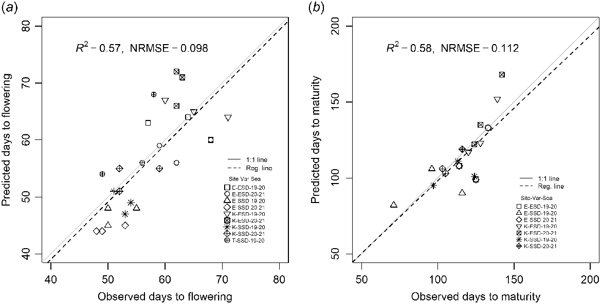
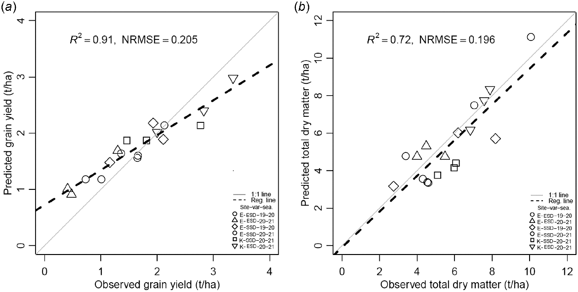
The performance of the APSIM pigeonpea model (ver. 7.10) was validated using flowering, maturity, yield and total dry matter data collected from agronomy experiments conducted for one super-short and one extra-short duration cultivar at three locations (Kingaroy, Toowoomba and Emerald) over two seasons. In these experiments, the number of days to 50% flowering ranged between 48 and 71 days, the number of days from sowing to maturity ranged from 71 and 142 days (Fig. 1), grain yield ranged from 0.4 to 3.3 t/ha and total dry matter from 2.75 t/ha to 10.06 t/ha (Fig. 2). The model’s performance appeared satisfactory, with an R2 of over 57% for time to flowering and maturity and an NRMSE of approximately 10% (Fig. 1). The NRMSE of yield and total dry matter was slightly more. R2 of simulated yield was 91% and 72% for the total dry matter at maturity. The model performance was further verified using independent data (not used for the calibration) collected in 2023 and appeared reasonably satisfactory, especially for yield (Fig. 3).
Comparison of observed and predicted number of days from sowing to flowering (a) and from sowing to maturity (b) at three locations (site), Kingaroy (K), Emerald (E) and Toowoomba (T), using super-short duration (SSD) and extra-short duration (ESD) cultivars (var) in the 2019–20 (19–20) and 2020–21 (20–21) seasons (sea). Maturity was not recorded at Toowoomba. The dashed line corresponds to a fitted linear relationship for each graph, while the solid line represents the 1:1 line.
Comparison of observed and predicted grain yield (a) and dry aboveground biomass (b) at maturity of super-short duration (SSD) and extra-short duration (ESD) cultivars at Kingaroy (K) in the 2020–21 season and Emerald (E) in the 2019–20 and 2020–21 seasons (sea). The dotted line corresponds to a linear relationship for each graph, while the solid line is the 1:1 line.
Observed and simulated data for (a) yield and (b) total dry matter (TDM) over time (days after sowing) at Kingaroy in 2023.
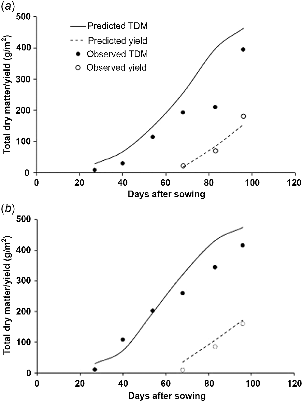
Though slightly higher, the simulated values of dry matter cut at different stages of super-short duration cultivars were within the acceptable range and flowering time could be predicted with high accuracy.
Spatial and temporal variation in yield and environmental similarity
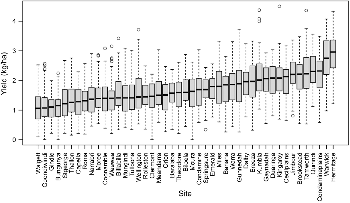
The model simulated a wide range of yields when applied to simulate 45 locations in the Australian northern grains region. The long-term average yields for the different locations varied between 1.1 t/ha for Walgett in NSW and 2.9 t/ha at Hermitage in Southeast Queensland, both being located at nearly similar latitudes but different longitudes (Fig. 4). The average coefficient of variation (CV) in yield across locations was between 28.9% for Emerald in Central Queensland and 57.2% for Walgett in New South Wales. The average CV was between 24.1 and 60.8% across seasons, with 2018 being the most variable season. At each location, the CV% for yield was negatively related to long-term average yield and average rainfall, while it was positively associated with the number of heat events.
Box plots of simulated yield of a super-short duration pigeonpea cultivar over 62 seasons in 45 locations across the Australia’s northern grains region. The locations were ranked based on median yield. For the boxplots, the middle line of the box represents the median, the upper and lower edges represent the 75th and 25th percentiles, the whiskers the 10th and 90th percentiles; and the dots outside the whiskers represent individual values outside this range.
Variation in average in-season rainfall across locations accounted for a smaller part (51%) of the variation across location-average yield (P < 0.01) but a larger part (71%) of the variation in seasonal yield (Fig. 5a, c). On average, an additional mm of in-season rainfall contributed to a 4.2 kg/ha increase in seasonal grain yield. The frequency of heat events (i.e. days with a maximum temperature >35°C) across locations varied between 2 and 20 days and accounted for nearly 73% (P ≤ 0.01) of the yield variation (Fig. 5b). However, across seasons, heat frequencies only accounted for 46% of the variation in yield (Fig. 5d). The frequency of combined heat-and-drought events (defined as the number of days with SDR of ≤0.3 and maximum temperature of ≥35°C) explained only slightly more variation (79%) in location-average yield than heat events alone. Each additional heat event contributed to an average yield loss of 2.9%.
Relationships between average yield and cumulated rainfall (a, c) and the number of heat events (b, d) averaged in (a, b) over 62 seasons (i.e. the average of all seasons for each specific location) or averaged in (c, d) across 45 locations (i.e. the average of all locations for a specific season). A heat event was defined as a day where the maximum temperature was equal to or greater than 35°C.
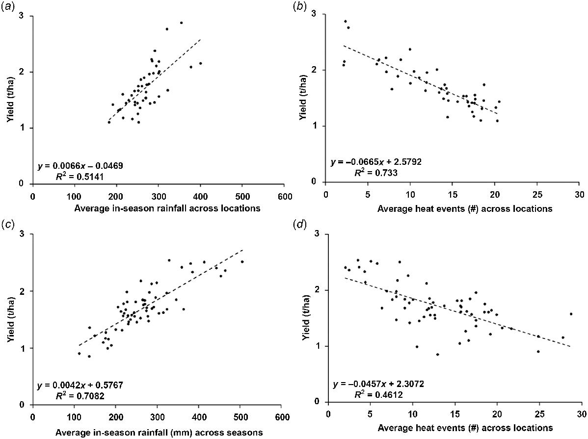
The number of in-season heat events and combined heat-and-drought events during the crop cycle were negatively associated with yield (r ≤ −0.86) and with longitude but had no substantial relationship with latitude (Table 3). Rainfall was significantly related to longitude (r = 0.56, P < 0.01). Individual drought events were strongly related to both latitude and longitude.
| Lat | Long | DEC1 | DEC2 | DEC3 | DEC4 | MTEC1 | MTEC2 | MTEC3 | MTEC4 | Heat | HtNDr | Drought | Rain | ||
|---|---|---|---|---|---|---|---|---|---|---|---|---|---|---|---|
| Lat | |||||||||||||||
| Long | −0.24 | ||||||||||||||
| DEC1 | 0.10 | 0.42 | |||||||||||||
| DEC2 | 0.42 | 0.44 | 0.27 | ||||||||||||
| DEC3 | −0.09 | −0.40 | −0.36 | −0.58 | |||||||||||
| DEC4 | −0.33 | −0.46 | −0.83 | −0.63 | 0.23 | ||||||||||
| MTEC1 | 0.35 | −0.86 | −0.50 | −0.42 | 0.29 | 0.55 | |||||||||
| MTEC2 | 0.06 | −0.02 | −0.46 | 0.32 | −0.13 | 0.22 | −0.02 | ||||||||
| MTEC3 | 0.02 | 0.00 | −0.33 | 0.40 | −0.19 | 0.08 | −0.10 | 0.71 | |||||||
| MTEC4 | −0.31 | 0.71 | 0.68 | 0.10 | −0.13 | −0.56 | −0.78 | −0.57 | −0.49 | ||||||
| Heat | 0.20 | −0.85 | −0.63 | −0.41 | 0.29 | 0.66 | 0.95 | 0.22 | 0.12 | −0.89 | |||||
| HtNDr | −0.07 | −0.73 | −0.74 | −0.57 | 0.32 | 0.84 | 0.86 | 0.19 | 0.06 | −0.79 | 0.94 | ||||
| Drought | −0.44 | −0.38 | −0.83 | −0.57 | 0.24 | 0.95 | 0.45 | 0.27 | 0.15 | −0.51 | 0.60 | 0.82 | |||
| Rain | 0.30 | 0.56 | 0.72 | 0.46 | −0.13 | −0.84 | −0.59 | −0.30 | −0.29 | 0.68 | −0.73 | −0.83 | −0.83 | ||
| Yield | −0.13 | 0.76 | 0.83 | 0.51 | −0.51 | −0.79 | −0.80 | −0.24 | −0.17 | 0.79 | −0.86 | −0.88 | −0.73 | 0.72 |
The values in bold are significant at 5% probability, n = 45.
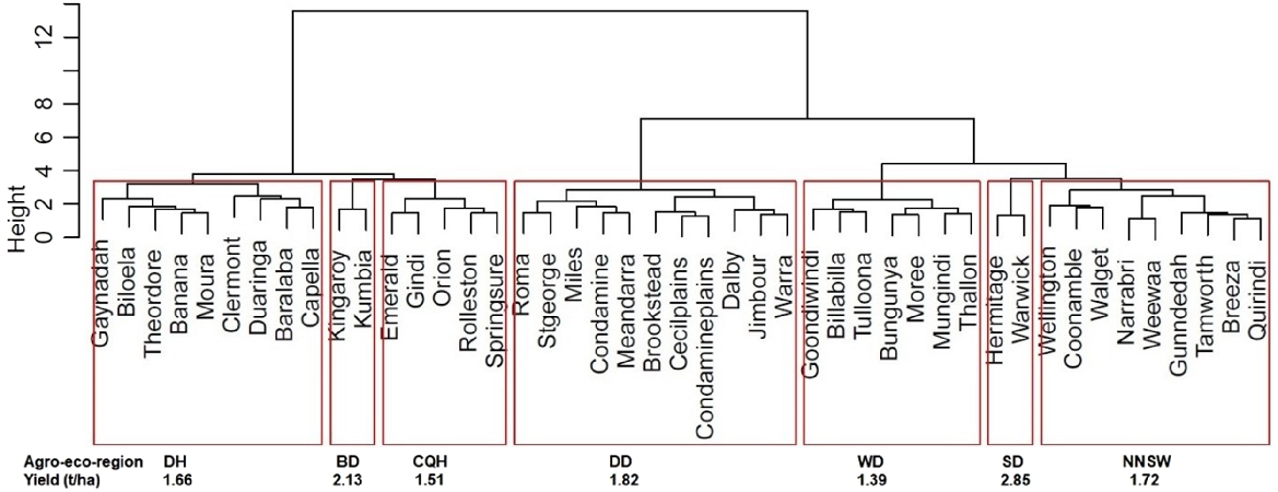
The location similarity analysis performed after transforming yield into percentiles to overcome the high magnitude effect in yield between locations (Fig. 6) showed no optimal number of clusters (data not shown). Based on expert knowledge, seven clusters were considered for this study, defining AERs. The grouping of locations across the seven AER was well represented in a dendrogram (Fig. 6) and geographically (Fig. 7). Approximately 60% of similarity in the yield percentile patterns could be captured within the seven AER (Fig. 6). To consider a larger level of similarity (i.e. more clusters), locations such as Dalby, Jimbour and Warra in the Darling Downs could be grouped together, and Brookstead, Cecil Plains and Condamine Plain could be grouped in separate clusters.
A dendrogram of locations highlighting groups of similar (agroecological regions) and dissimilar locations in terms of percentiles of seasonal yield as well as the long-term average yield within each agroecological region (below the dendrogram) for a super-short duration pigeonpea cultivar. The joining height of clusters represents the degree of dissimilarity. The seven clusters captured approximately 60% variability. The agroecological regions are DC, Dawson Callide; WD, Western Downs; NNSW, Northern New South Wales; DD, Darling Downs; CQH, Central Queensland Highlands; SD, Southern Downs; and BD, Burnett District.
Clustering of locations based on long-term averaged yield (a) and percentile ranks (b) developed for a super-short duration pigeonpea cultivar. The agroecological regions (i.e. clusters) are generally more contiguous and compact when developed using percentile ranks (b) rather than when based on temporal changes in actual yield of the locations (a). They are also consistent with agroecologies reported by local experts. The agroecological regions are DC, Dawson Callide; WD, Western Downs; NNSW, Northern New South Wales; DD, Darling Downs; CQH, Central Queensland Highlands; SD, Southern Downs; and BD, Burnett District.
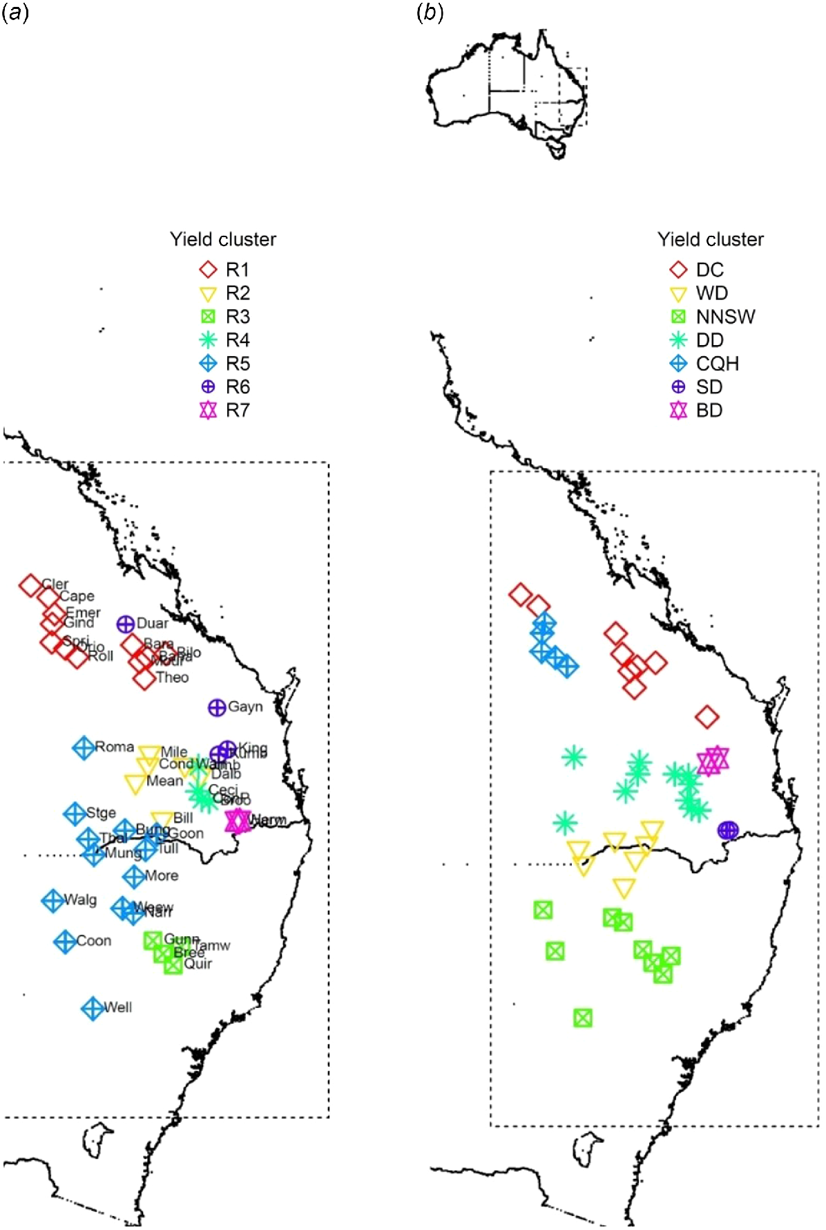
When temporal changes in yield without transformation into percentile were clustered, non-contiguous locations were clustered together, e.g. in cluster R6 (Fig. 7a). Also, locations from the Darling Downs were clustered in one cluster using the percentile criteria, whereas they were in three clusters using the yield criteria. Similarly, the yield-cluster equivalent of the Dawson Callide yield-percentile cluster (i.e. R6) extended up to the Burnett District.
In contrast, the clustering of seasonal changes in yield percentiles resulted in a more compact grouping of locations (Fig. 7b). With this method, locations within each AER were more contiguous.
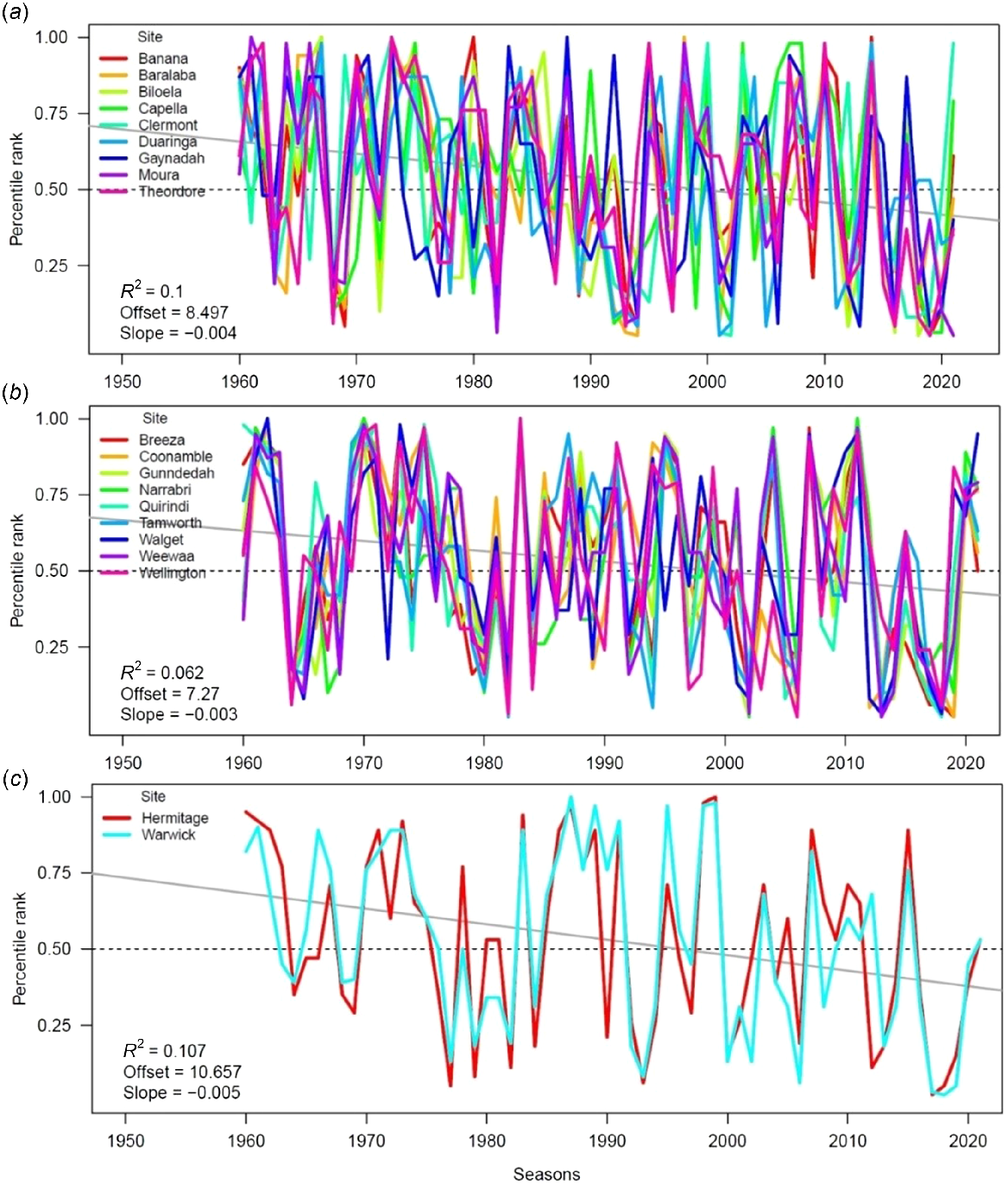
Further, when plotted over time, yield percentiles changed cohesively for the different locations of each cluster compared to across clusters (Fig. 8). A declining trend in yield-percentile over 1960–2021 was observed for all AERs, with significant change detected in Dawson Callide, Southern Downs and Northern New South Wales AERs (Fig. 8).
Examples of synchronous patterns of yield percentiles over time for three agroecological regions in Dawson Callide (a), Northern New South Wales (b) and Southern Downs (c). With time, all three agroecological regions had a significant downward trend in percentiles (solid grey line). Similar changes were also observed in other agroecological regions but were not significant at a level of 0.05.
Drought and heat environments classes and their frequencies across agroecological regions
Heat and drought stress commonly affect yield differently depending upon the phenological stage when they occur. As these stresses can be responsible for substantial spatial and temporal variations in grain yield of pigeonpea in the studied region, their patterns and their frequencies of occurrence were characterised. A cluster analysis was performed for both (1) water SDR as an indicator of drought and (2) maximum temperatures as an indicator of stress for every 100°Cd segment before and after flowering. Analysing 27 900 data points (i.e. 62 seasons, 45 locations and 10 segments of 100°Cd) of a super-short duration cultivar revealed four significant drought environment classes (DEC1–4) and four major types of maximum temperature environment classes (MTEC1–4), with varying frequencies of occurrence across seven agroecological regions (Table 4).
| Agroecological region | Drought env. class (DEC) | Maximum temp. env. class (MTEC) | |||||||
|---|---|---|---|---|---|---|---|---|---|
| DEC1 | DEC2 | DEC3 | DEC4 | MTEC1 | MTEC2 | MTEC3 | MTEC4 | ||
| Dawson Callide | 22.9 | 32.2 | 15.8 | 29.0 | 38.7 | 27.6 | 30.3 | 3.4 | |
| Western Downs | 14.1 | 15.7 | 20.3 | 50.0 | 42.9 | 26.5 | 22.8 | 7.8 | |
| Northern-NSW | 22.0 | 18.1 | 20.3 | 39.6 | 24.6 | 25.4 | 26.7 | 23.3 | |
| Darling Downs | 24.2 | 28.6 | 17.3 | 29.9 | 18.5 | 31.2 | 29.3 | 21.0 | |
| CQ-Highlands | 27.4 | 22.9 | 21.3 | 28.4 | 51.3 | 24.2 | 22.9 | 1.6 | |
| Southern Downs | 61.3 | 20.2 | 10.5 | 8.1 | 0.0 | 4.0 | 4.0 | 91.9 | |
| South Burnett | 33.1 | 23.4 | 27.4 | 16.1 | 0.0 | 8.9 | 4.0 | 87.1 | |
| Mean | 24.3 | 24.0 | 18.6 | 33.0 | 29.5 | 25.6 | 25.0 | 19.8 | |
The four DECs varied in the timing and intensity of the water stress experienced by the crop (Fig. 9a). Environments from DEC1 – a low or no-stress type, were characterised by higher SDR than the other stress types. They occurred with an average frequency of 24.3% and had an average yield of 2.20 t/ha with a CV of 31%. DEC1 environment occurred with the highest frequency (54.8 to 67.7%) in the Southern Downs AER. The frequency of DEC1 was positively associated with yield (r = 0.83, P < 0.01) (Table 3). DEC1 frequency was also positively related to longitude, though weakly.
Main in-season patterns of drought (DEC, a) and their factor loadings (b), and maximum temperature (MTEC, c) and their factor loadings (d). The effects of drought and maximum temperature classes on yield are shown in inset charts in (a) and (c). The clusters representing different agroecological regions in charts (b) and (d) are DC, Dawson Callide; WD,Western Downs; NNSW, Northern New South Wales; DD, Darling Downs; CQH, Central Queensland Highlands; SD, Southern Downs; and BD, Burnett District.
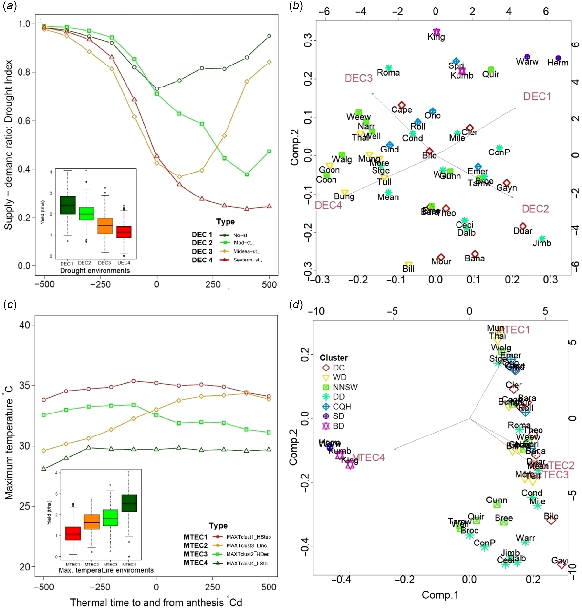
DEC2 – a moderate-stress type, occurred with a frequency of 24.4%. DEC2 was characterised by a water-stress index that declined from the pre-flowering period until close to maturity. DEC2 environments had a simulated yield of 2.0 t/ha, with a CV of 23.4%. The frequency of DEC2, like DEC1, was positively associated with yield (r = 0.51, P < 0.01). DEC2 frequency also had a weak positive association with latitude and longitude.
DEC3 – a severe mid-season type of stress, occurred with a frequency of 18.6%. DEC3 was characterised by a decline in the water stress index during the vegetative period to approximately 250°Cd after flowering, with a substantial release after that. The average yield associated with DEC3 was 1.44 t/ha, with a CV of 37.7%. The frequency of environments from DEC3 was negatively associated with yield (r = −0.51, P < 0.01) (Table 3). The DEC3 frequency was unrelated to latitude and longitude (r < 0.21).
DEC4 – a severe mid-to-end season stress type, occurred with a frequency of 30.2%. DEC4 was characterised by a decline in the water stress index during the vegetative period, similar to DEC3, but with no release during grain filling. The water stress index typically declined to be <0.3 towards crop maturity. The average yield associated with DEC4 was 0.92 t/ha with a CV of 37.4%. The frequency DEC4 was negatively associated with yield (r = 0.79, P < 0.01). DEC4 frequency was negatively related to longitude (r = −0.46, P < 0.01).
The combined frequency of severe DEC3 and DEC4 drought types, negatively associated with yield, was 51.6% in the northern grains region. A principal component analysis indicates that these environments were mainly found in Northern New South Wales and the Western Downs location clusters (Fig. 9b).
Four major types of maximum temperature environments (MTEC1–4) were identified (Fig. 9c) with varying impacts on yield depending mainly on post-flowering heat stress. MTEC1 occurred at a frequency of 29.5%, MTEC2 25.0%, MTEC3 25.6% and MTEC4 19.8% (Table 4). The average simulated yield (± s.e.) for MTEC1 environments was 1.0 ± 0.46 t/ha, 1.63 ± 0.47 t/ha for MTEC2, 1.83 ± 0.53 for MTEC3 and 2.53 ± 0.48 for MTEC4.
Grain yield was positively correlated with the MTEC4 frequency of occurrence (r = 0.794, P < 0.01) and negatively correlated (r = 0.800, P < 0.01) with MTEC1 frequencies of occurrence, while no significant relationship was found for MTEC2 and MTEC3 (Table 3). MTEC1 was negatively related to longitude (r = 0.86, P < 0.01) and positively associated with latitude (r = 0.35, P < 0.01).
The principal component analysis indicated a prominent presence of MTEC1 and MTEC2 in Western Downs, Central Highland and Dawson Callide AER (Fig. 9d). In contrast, MTEC4 was more pronounced in Southern Downs and Burnett AER (Fig. 9d). Severe MTEC1 and MTEC2 environments were more common in the Central Queensland Highlands, New South Wales and Western Downs AER. The principal component analysis also revealed this dominant distribution of the most-severe MTEC1 (Fig. 9d). Of the 45 locations, 16 had very low frequencies of severe MTEC1 and MTEC2 types of temperature environments (Table 4).
Discussion
Yield potential of super-short duration pigeonpea
There is little documentation of pigeonpea cropping trials in the Australia’s northern grains region (NGR), which has a sub-tropical climate with summer-dominant rainfall. To the best of our knowledge, this study is the first attempt to comprehensively evaluate the suitability of pigeonpea in the summer season of the NGR with crop modelling. The APSIM pigeonpea model required adjustment of a few parameters related to crop phenology, radiation use efficiency, transpiration efficiency, growth and daily dry matter partitioning into yield (Table S1), and the predictive accuracy comparable to earlier validation reported for pigeonpea (Robertson et al. 2001; Rao et al. 2013). Changes made for the RUE were consistent with higher values observed under rainout shelters, where transient waterlogging known to impact this trait adversely (Milroy and Bange 2013) was avoided due to controlled application of water (Nam et al. 1998). Changes in the crop coefficient for transpiration use efficiency may have been necessitated due to genetic improvement of modern genotypes as observed for wheat (Triticum aestivum) (Fletcher and Chenu 2015), and/or increased atmospheric carbon dioxide concentration (Leakey et al. 2019). This should be examined in future experiments. The calibrated model could accurately simulate growth and development accross the tested locations and planting times, with some small over-predictions of low yields and small under-predictions of high yields. Those minor discrepancies are common in some legumes such as chickpea (Cicer arietinum) (Robertson et al. 2002). Although further research may be necessary to further improve the model, we deemed the bias acceptable to characterise pigeonpea growing environments.
Simulated results suggest that approximately three-fold variation in water-limited yield is due to differences across seasons and locations. Such variability in yield was consistent with the observed performance of other related crop species grown in the region, including mungbean and chickpea. When searching for the main limiting abiotic factors responsible for yield variation, we found that in-season rainfall accounted for approximately 71% of the temporal (seasonal) and 51% of the spatial (locational) variation in yield (Fig. 4a). In contrast, heat events across locations with a daily maximum temperature >35°C accounted for 46% of seasonal variation and 74% of spatial variation in yield (Fig. 4a). In wheat, approximately 43% of the variability in crop yield across Australia was reported to be explained by climatic factors, of which rainfall and temperature were essential components. In the current study, frequencies of heat-and-drought events together explained nearly 77% of yield variation. Of this, temperature alone appeared as the dominant factor, accounting for almost 73% of the variation in yield. According to a Grains Research and Development Corporation (GRDC) estimate, Australia suffers from a AUD1.1 billion annual loss in grain yield related to high temperature of all broad acre crops already grown in Australia. Pigeonpea being a summer crop, the impacts of temperatures are likely to be greater than for winter crops such as wheat. However, pigeonpea was found to be more resilient to increase in temperature among summer crops than sorghum (Sorghum bicolor), pearl millet (Pennisetum glaucum), peanut (Arachis hypogaea) and maize (Zea mays) (Dimes et al. 2008; Jat et al. 2012). In addition, targeted short-season pigeonpea cultivars cultivated as monocropping culture in Australia could pose an additional risk as they would be grown at higher planting densities. Hence, despite the reputation of pigeonpea as a more resilient crop in rainfed/dryland farming systems, improvements in its heat tolerance may still be required.
Surprisingly, seasonal variation in yield was less related to frequencies of heat events than rainfall (Fig. 5). Rainfall amount and distribution likely influenced the timings and severity of drought and heat stresses. This effect was supported by a negative correlation (−0.73) between rainfalls and heat stress frequencies (Table 3). Further, correlation analysis suggested strong effects of longitude on rainfalls and frequencies of heat events. A relationship of latitude and longitude with rainfalls, drought and heat-event frequencies indicated that these factors and the location could consistently affect the pigeonpea adaptation.
Furthermore, climate change could increase extreme temperature events and decrease or increase rainfall. These changes may affect season-average yield, location-average yield, or both. Long-term climate projections suggest that there is unlikely to be a major shift in summer season rainfall amount in eastern Australia. Hence, grain yields may decline markedly with the projected increase in maximum temperatures, even if rainfall may not be affected much. How changes in these climatic factors would change yielding patterns could be examined, also looking at possible adaptations, for instance, in sowing dates and maturity types (Collins and Chenu 2021). In the current study, as the aim is to evaluate the potential to establish a new crop, this information would be valuable to assess future trends and potential for breeding and agronomic adaptation.
In examining variations in climatic environments, it is crucial to consider both spatial and temporal variation. Breeders generally prefer to focus on improving the spatial adaptation of crops (i.e. in terms of locations). In contrast, individual growers are more interested in performance across seasons at their location. Hence to meet both requirements, environment similarity must be looked at in both spatial and temporal terms.
Environment similarity is conventionally determined through statistical analysis of genotypes, environments, crop management practices, and their interactions. This approach, however, often ignores the impact of temporal variation and the long-term stability of performance as the trials are conducted over a limited period. Identifying environment similarity that captures spatial and temporal variability to determine the similarity of environments is valuable from a breeding perspective that supports both the community of growers and individual growers. Crop modelling allowed pigeonpea’s performance to be evaluated comprehensively across locations and seasons. Clustering for environmental homogeneity based on yield percentiles over 62 seasons identified seven agroecological zones with similar ecological patterns. These agroecological zones differed substantially in terms of drought and heat types frequencies.
A few studies have previously simulated yield directly to identify similarities between locations in regions with variable climates (Aggarwal 1993; Chauhan et al. 2008, 2013; Seyoum et al. 2017). However, such an approach may not be relevant for variable environments. In the current study, clustering environments based on absolute yield values led to grouping locations geographically far apart (Fig. 6a). This may be why simulated yield has had limited use in identifying similarities across locations. This may even be more glaring in breeding trials as such trials are typically conducted for a limited number of seasons. By contrast, when grouping locations from the current study based on seasonal variations in yield percentile, locations grouped as environmentally similar in agroecological regions were geographically contiguous (Fig. 6b) and meaningful to local agronomists who could see some value in such grouping.
The locations of the different agroecological zones identified were further characterised by heat and drought stress frequencies (Fig. 8). Each agroecological zone tended to have one to two dominating maximum temperature environments (Fig. 8d). Regarding the most severe stresses, it appeared that severely stressed MTEC1 and MTEC2 type environments were more common in Central Queensland, New South Wales and Western Downs, whereas yield-reducing DEC4 environments were more frequent in Western Downs and New South Wales clusters.
Implications for the future of the pigeonpea industry
This study identified seven Australian agroecological regions where pigeonpea could be cultivated. Similar frequencies of abiotic stresses characterised each agroecological region within member locations. While only 45 key locations were studied, other locations from the area are likely to have similar environments to the neatest studied locations and be part of the same agroecological region. Simulations could be quickly run and analysed if climatic data are available to confirm this.
In some agroecological regions such as Western Downs, Central Queensland Highlands and Northern New South Wales, greater heat tolerance may be required to achieve higher and more stable production. Greater drought tolerance may be necessary to stabilise yield across seasons, especially in low rainfall environments. Identifying climatically disparate environments represented by different agroecological regions could offer an opportunity to develop region-specific cultivars and agronomy. For instance, pigeonpea cultivars tolerant to heat and drought could be introduced from other breeding programs and bred locally for the marginal agroecological areas in the Western Downs, Northern NSW and Central Queensland Highlands. Further, the proposed method could be applied to other pigeonpea-producing regions worldwide to identify agroecological zones with similar stress patterns as found in the Australian northern grains region, thus facilitating meaningful importation of germplasm with interesting adaptation to Australia.
Identifying and characterising similarities between environments for crucial constraints should arguably be the first step to considering the prospects of a new crop and setting up the breeding objective -unless the crop has other issues related to biotic stress. In the past, pest problems, which overwhelmed the local pigeonpea crops, seem to have become more manageable due to the development of new, more effective pesticides (T. Volp, pers. comm.). Past research on the crop has mainly focused on breeding new cultivars with a relative lack of understanding of the possible agro-climatic environments and agronomy required in different locations. The current study is one of the new approaches implemented to resurrect the Australian pigeonpea industry and precedes any recent breeding efforts for this crop.
Conclusions
This research was focused on determining environmental similarities for pigeonpea in Australia using the APSIM model. The method considers both spatial and temporal variations, making it more reliable than traditional approaches that are based on average yield obtained over a few seasons of trials. This study bridges the knowledge gap about pigeonpea’s agro-climatic adaptation in the Australian northern grains region for new super-short duration cultivars. Analysing the frequency of abiotic stresses makes it possible to identify yield constraints within each agroecological region, prioritise testing locations, and inform future pre-breeding and breeding studies. This approach also helps understand how climate affects pigeonpea production in agroecological regions.
The results suggest that pigeonpea has the potential to become a primary pulse rotation crop during the summer season in the northern grains region of Australia. Efforts to establish the pigeonpea industry could focus on locations with a yield potential of approximately 2 t/ha, such as in the favourable agroecological zones of South Burnett and Darling Downs. Alternatively, pigeonpea cultivars tolerant to heat and drought could be used in more marginal areas like Western Downs, Emerald and Northern New South Wales agroecological regions. The approach developed in this study is now being used to inform local pulse breeding programs and could be applied to other crops and regions.
Data availability
The data that support this study can be shared upon reasonable request to the corresponding author.
Declaration of funding
This research was funded by the Department of Agriculture and Fisheries under a pigeonpea initiative (unnumbered).
Author contributions
YSC, RW conceived the study. YSC, SK, DS, PA, TF conducted the fieldwork. YSC drafted the manuscript with insightful discussion and input from KC, RW and other co-authors.
Acknowledgements
The authors thank the Australian Grains Gene Bank and the International Crops Research Institute for the Semi-Arid Tropics (ICRISAT) for the seed of new germplasm lines for testing the model and the APSIM initiative for providing the APSIM software.
References
Abram NJ, Henley BJ, Sen Gupta A, Lippmann TJR, Clarke H, Dowdy AJ, Sharples JJ, Nolan RH, Zhang T, Wooster MJ, Wurtzel JB, Meissner KJ, Pitman AJ, Ukkola AM, Murphy BP, Tapper NJ, Boer MM (2021) Connections of climate change and variability to large and extreme forest fires in southeast Australia. Communications Earth & Environment 2, 8.
| Crossref | Google Scholar |
Cattell RB (1966) The scree test for the number of factors. Multivariate Behavioral Research 1, 245-276.
| Crossref | Google Scholar |
Chapman SC (2008) Use of crop models to understand genotype by environment interactions for drought in real-world and simulated plant breeding trials. Euphytica 161, 195-208.
| Crossref | Google Scholar |
Chapman SC, Hammer GL, Butler D, Cooper M (2000) Genotype by environment interactions affecting grain sorghum. III. Temporal sequences and spatial patterns in the target population of environments. Australian Journal of Agricultural Research 51, 223-234.
| Crossref | Google Scholar |
Chauhan YS, Rachaputi RCN (2014) Defining agro-ecological regions for field crops in variable target production environments: a case study on mungbean in the northern grains region of Australia. Agricultural and Forest Meteorology 194, 207-217.
| Crossref | Google Scholar |
Chauhan YS, Johansen C, Moon J-K, Lee Y-H, Lee S-H (2002) Photoperiod responses of extra-short-duration pigeonpea lines developed at different latitudes. Crop Science 42, 1139-1146.
| Crossref | Google Scholar |
Chauhan Y, Wright G, Rachaputi N, McCosker K (2008) Identifying chickpea homoclimes using the APSIM chickpea model. Australian Journal of Agricultural Research 59, 260-269.
| Crossref | Google Scholar |
Chauhan YS, Solomon KF, Rodriguez D (2013) Characterization of north-eastern Australian environments using APSIM for increasing rainfed maize production. Field Crops Research 144, 245-255.
| Crossref | Google Scholar |
Chauhan Y, Allard S, Williams R, Williams B, Mundree S, Chenu K, Rachaputi NC (2017) Characterisation of chickpea cropping systems in Australia for major abiotic production constraints. Field Crops Research 204, 120-134.
| Crossref | Google Scholar |
Chauhan Y, Krosch S, Sands D, Agius P, Fredricks T, Borgognone M, Ryan M, Williams R (2022) Agronomic characteristics of pigeonpea as a summer crop for Queensland. In ‘Proceedings of the 20th Agronomy Australia Conference’, Toowoomba, Qld. (Australian Society of Agronomy: Warragul, Vic., Australia). Available at https://www.agronomyaustraliaproceedings.org/images/sampledata/2022/Pulses/ASAchauhan_y_378s.pdf
Chenu K, Cooper M, Hammer GL, Mathews KL, Dreccer MF, Chapman SC (2011) Environment characterization as an aid to wheat improvement: interpreting genotype–environment interactions by modelling water-deficit patterns in North-Eastern Australia. Journal of Experimental Botany 62, 1743-1755.
| Crossref | Google Scholar |
Chenu K, Deihimfard R, Chapman SC (2013) Large-scale characterization of drought pattern: a continent-wide modelling approach applied to the Australian wheatbelt–spatial and temporal trends. New Phytologist 198, 801-820.
| Crossref | Google Scholar |
Collins B, Chenu K (2021) Improving productivity of Australian wheat by adapting sowing date and genotype phenology to future climate. Climate Risk Management 32, 100300.
| Crossref | Google Scholar |
Cooper M, Messina CD (2021) Can we harness “Enviromics” to accelerate crop improvement by integrating breeding and agronomy? Frontiers in Plant Science 12, 735143.
| Crossref | Google Scholar |
Cooper M, Delacy IH, Byth DE, Woodruff DR (1993) Predicting grain yield in Australian environments using data from CIMMYT international wheat performance trials. 2. The application of classification to identify environmental relationships which exploit correlated response to selection. Field Crops Research 32, 323-342.
| Crossref | Google Scholar |
Dimes JP, Cooper P, Rao K (2008) Climate change impact on crop productivity in the semi-arid tropics of Zimbabwe in the 21st century. In ‘Proceedings of the Workshop on Increasing the Productivity and Sustainability of Rainfed Cropping Systems of Poor Smallholder Farmers’, 22–25 September 2008. Tamale, Ghana. pp. 189–198. (The CGIAR Challenge Program on Water and Food: Sri Lanka)
Gauch HG, Jr., Zobel RW (1997) Identifying mega-environments and targeting genotypes. Crop Science 37, 311-326.
| Crossref | Google Scholar |
Geetika G, Hammer G, Smith M, Singh V, Collins M, Mellor V, Wenham K, Rachaputi RCN (2022) Quantifying physiological determinants of potential yield in mungbean (Vigna radiata (L.) Wilczek). Field Crops Research 287, 108648.
| Crossref | Google Scholar |
Harrison MT, Tardieu F, Dong Z, Messina CD, Hammer GL (2014) Characterizing drought stress and trait influence on maize yield under current and future conditions. Global Change Biology 20, 867-878.
| Crossref | Google Scholar |
Hodson DP, White JW (2007) Use of spatial analyses for global characterization of wheat-based production systems. The Journal of Agricultural Science 145, 115.
| Crossref | Google Scholar |
Holzworth DP, Huth NI, deVoil PG, Zurcher EJ, Herrmann NI, McLean G, Chenu K, van Oosterom EJ, Snow V, Murphy C, Moore AD, Brown H, Whish JPM, Verrall S, Fainges J, Bell LW, Peake AS, Poulton PL, Hochman Z, Thorburn PJ, Gaydon DS, Dalgliesh NP, Rodriguez D, Cox H, Chapman S, Doherty A, Teixeira E, Sharp J, Cichota R, Vogeler I, Li FY, Wang E, Hammer GL, Robertson MJ, Dimes JP, Whitbread AM, Hunt J, van Rees H, McClelland T, Carberry PS, Hargreaves JNG, MacLeod N, McDonald C, Harsdorf J, Wedgwood S, Keating BA (2014) APSIM – evolution towards a new generation of agricultural systems simulation. Environmental Modelling & Software 62, 327-350.
| Crossref | Google Scholar |
Jat RA, Craufurd P, Sahrawat KL, Wani SP (2012) Climate change and resilient dryland systems: experiences of ICRISAT in Asia and Africa. Current Science 102, 1650-1659.
| Google Scholar |
Jeffrey SJ, Carter JO, Moodie KB, Beswick AR (2001) Using spatial interpolation to construct a comprehensive archive of Australian climate data. Environmental Modelling & Software 16, 309-330.
| Crossref | Google Scholar |
Leakey ADB, Ferguson JN, Pignon CP, Wu A, Jin Z, Hammer GL, Lobell DB (2019) Water use efficiency as a constraint and target for improving the resilience and productivity of C3 and C4 crops. Annual Review of Plant Biology 70, 781-808.
| Crossref | Google Scholar |
Meinke H, Stone RC (2005) Seasonal and inter-annual climate forecasting: the new tool for increasing preparedness to climate variability and change in agricultural planning and operations. Climatic Change 70, 221-253.
| Crossref | Google Scholar |
Milroy SP, Bange MP (2013) Reduction in radiation use efficiency of cotton (Gossypium hirsutum L.) under repeated transient waterlogging in the field. Field Crops Research 140, 51-58.
| Crossref | Google Scholar |
Nam NH, Subbarao GV, Chauhan YS, Johansen C (1998) Importance of canopy attributes in determining dry matter accumulation of pigeonpea under contrasting moisture regimes. Crop science 38, 955-961.
| Crossref | Google Scholar |
Rahimi-Moghaddam S, Deihimfard R, Nazari MR, Mohammadi-Ahmadmahmoudi E, Chenu K (2023) Understanding wheat growth and the seasonal climatic characteristics of major drought patterns occurring in cold dryland environments from Iran. European Journal of Agronomy 145, 126772.
| Crossref | Google Scholar |
Rao AK, Wani SP, Srinivas K, Singh P, Bairagi SD, Ramadevi O (2013) Assessing impacts of projected climate on pigeonpea crop at Gulbarga. Journal of Agrometeorology 15, 32-37.
| Google Scholar |
Ray DK, Gerber JS, MacDonald GK, West PC (2015) Climate variation explains a third of global crop yield variability. Nature Communications 6, 5989.
| Crossref | Google Scholar |
Robertson MJ, Carberry PS, Chauhan YS, Ranganathan R, O’leary GJ (2001) Predicting growth and development of pigeonpea: a simulation model. Field Crops Research 71, 195-210.
| Crossref | Google Scholar |
Robertson MJ, Carberry PS, Huth NI, Turpin JE, Probert ME, Poulton PL, Bell M, Wright GC, Yeates SJ, Brinsmead RB (2002) Simulation of growth and development of diverse legume species in APSIM. Australian Journal of Agricultural Research 53, 429-446.
| Crossref | Google Scholar |
Saxena K, Choudhary AK, Srivastava RK, Bohra A, Saxena RK, Varshney RK (2019) Origin of early maturing pigeonpea germplasm and its impact on adaptation and cropping systems. Plant Breeding 138, 243-251.
| Crossref | Google Scholar |
Seyoum S, Chauhan Y, Rachaputi R, Fekybelu S, Prasanna B (2017) Characterising production environments for maize in eastern and southern Africa using the APSIM Model. Agricultural and Forest Meteorology 247, 445-453.
| Crossref | Google Scholar |
Thornton PK, Ericksen PJ, Herrero M, Challinor AJ (2014) Climate variability and vulnerability to climate change: a review. Global Change Biology 20, 3313-3328.
| Crossref | Google Scholar |
Vales MI, Srivastava RK, Sultana R, Singh S, Singh I, Singh G, Patil SB, Saxena KB (2012) Breeding for earliness in pigeonpea: development of new determinate and nondeterminate lines. Crop Science 52, 2507-2516.
| Crossref | Google Scholar |
Vázquez DP, Gianoli E, Morris WF, Bozinovic F (2017) Ecological and evolutionary impacts of changing climatic variability. Biological Reviews 92, 22-42.
| Crossref | Google Scholar |
White DH, Lubulwa GA, Menz K, Zuo H, Wint W, Slingenbergh J (2001) Agro-climatic classification systems for estimating the global distribution of livestock numbers and commodities. Environment International 27, 181-187.
| Crossref | Google Scholar |