

Weed recognition using deep learning techniques on class-imbalanced imagery
A. S. M. Mahmudul Hasan A B , Ferdous Sohel A B * , Dean Diepeveen B C , Hamid Laga A D and Michael G. K. Jones B
A Information Technology, Murdoch University, Murdoch, WA 6150, Australia.
B Centre for Crop and Food Innovation, Food Futures Institute, Murdoch University, Murdoch, WA 6150, Australia.
C Department of Primary Industries and Regional Development, South Perth, WA 6151, Australia.
D Centre of Biosecurity and One Health, Harry Butler Institute, Murdoch University, Murdoch University, Murdoch, WA 6150, Australia.
Crop & Pasture Science - https://doi.org/10.1071/CP21626
Submitted: 9 August 2021 Accepted: 9 December 2021 Published online: 11 April 2022
© 2022 The Author(s) (or their employer(s)). Published by CSIRO Publishing. This is an open access article distributed under the Creative Commons Attribution-NonCommercial-NoDerivatives 4.0 International License (CC BY-NC-ND)
Abstract
Context: Most weed species can adversely impact agricultural productivity by competing for nutrients required by high-value crops. Manual weeding is not practical for large cropping areas. Many studies have been undertaken to develop automatic weed management systems for agricultural crops. In this process, one of the major tasks is to recognise the weeds from images. However, weed recognition is a challenging task. It is because weed and crop plants can be similar in colour, texture and shape which can be exacerbated further by the imaging conditions, geographic or weather conditions when the images are recorded. Advanced machine learning techniques can be used to recognise weeds from imagery.
Aims: In this paper, we have investigated five state-of-the-art deep neural networks, namely VGG16, ResNet-50, Inception-V3, Inception-ResNet-v2 and MobileNetV2, and evaluated their performance for weed recognition.
Methods: We have used several experimental settings and multiple dataset combinations. In particular, we constructed a large weed-crop dataset by combining several smaller datasets, mitigating class imbalance by data augmentation, and using this dataset in benchmarking the deep neural networks. We investigated the use of transfer learning techniques by preserving the pre-trained weights for extracting the features and fine-tuning them using the images of crop and weed datasets.
Key results: We found that VGG16 performed better than others on small-scale datasets, while ResNet-50 performed better than other deep networks on the large combined dataset.
Conclusions: This research shows that data augmentation and fine tuning techniques improve the performance of deep learning models for classifying crop and weed images.
Implications: This research evaluates the performance of several deep learning models and offers directions for using the most appropriate models as well as highlights the need for a large scale benchmark weed dataset.
Keywords: crop and weed classification, digital agriculture, Inception-ResNet-V2, Inception-V3, machine learning, MobileNetV2, precision agriculture, ResNet-50, VGG16.
Introduction
Weeds in crops compete for water, nutrients, space and light, and may decrease product quality (Iqbal et al. 2019). Their control, using a range of herbicides, constitutes a significant part of current agricultural practices. In Australia, weed control costs in grain production is estimated at AUD4.8 billion per annum. These costs include weed control and the cost of lost production (McLeod 2018).
The most widely used methods for controlling weeds are chemical-based, where herbicides are applied at an early growth stage of the crop (López-Granados 2011; Harker and O’Donovan 2013). Although the weeds spread in small patches in crops, herbicides are usually applied uniformly throughout the agricultural field. While such an approach works reasonably well against weeds, it also affects the crops. A report from the European Food Safety Authority (EFSA) shows that most of the unprocessed agricultural produces contain harmful substances originating from herbicides (Medina-Pastor and Triacchini 2020).
Recommended rates of herbicide application are expensive and may also be detrimental to the environment. Thus, new methods that can be used to identify weeds in crops, and then selectively apply herbicides on the weeds, or other methods to control weeds, will reduce production costs to the farmers and benefit the environment. Technologies that enable the rapid discrimination of weeds in crops are now becoming available (Tian et al. 2020).
Recent advances in Deep Learning (DL) have revolutionised the field of Machine Learning (ML). DL has made a significant impact in the area of computer vision by learning features and tasks directly from audio, images or text data without human intervention or predefined rules (Dargan et al. 2020). For image classification, DL methods outperform humans and traditional ML methods in accuracy and speed (Steinberg 2017). In addition, the availability of computers with powerful GPUs, coupled with the availability of large amounts of labelled data, enable the efficient training of DL models.
As for other computer vision and image analysis problems, digital agriculture and digital farming also benefits from the recent advances in deep learning. DL techniques have been applied for weed and crop management, weed detection, localisation and classification, field conditions and livestock monitoring (Kamilaris and Prenafeta-Boldú 2018).
ML techniques have been used in commercial solutions to combat weeds. ‘Robocrop Spot Sprayer’ (Robocrop Spot sprayer: weed removal 2018) is a video analysis-based autonomous selective spraying system that can identify potatoes (Solanum tuberosum L.) grown in carrots (Daucus carota L. subsp. sativus), parsnips (Pastinaca sativa L.), onions (Allium cepa L.) or leeks (Allium porrum L.). ‘WeedSeeker sprayer’ (WeedSeeker 2 Spot Spray System n.d.) is a near-infrared reflectance sensor-based system that detects the green component in the field. The machine sprays herbicides only on the plants while reducing the amount of herbicide. Similar technology is offered by a herbicide spraying system known as ‘WEED-IT’. It can target all green plants on the soil. A fundamental problem with these systems is that they are non-selective of crops or weeds. Therefore the ability to discriminate between crops and weeds is important.
Further development of autonomous weed control systems can be beneficial both economically and environmentally. Labour costs can be reduced by using a machine to identify and remove weeds. Selective spraying can also minimise the amount of herbicides applied (Lameski et al. 2018). The success of an autonomous weed control system will depend on four core modules: (1) weed detection and recognition; (2) mapping; (3) guidance; and (4) weed control (Olsen et al. 2019). This paper focuses on the first module: weed detection and recognition, which is a challenging task (Slaughter et al. 2008). This is because both weeds and crop plants often exhibit similar colours, textures and shapes. Furthermore, the visual properties of both weeds and crop plants can vary depending on the growth stage, lighting conditions, environments and geographical locations (Jensen et al. 2020; Hasan et al. 2021). Also, weeds and crops, exhibit high inter-class similarity as well as high intra-class dissimilarity. The lack of large-scale crop weed datasets is a fundamental problem for DL-based solutions.
There are many approaches to recognise weed and crop classes from images (Wäldchen and Mäder 2018). High accuracy can be obtained for weed classification using DL techniques (Kamilaris and Prenafeta-Boldú 2018) whereas Chavan and Nandedkar (2018) used Convolutional Neural Network (CNN) models to classify weeds and crop plants. Teimouri et al. (2018) used DL for the classification of weed species and the estimation of growth stages, with an average classification accuracy of 70% and 78% for growth stage estimation.
As a general rule, the accuracy of the methods used for the classification of weed species decreases in multi-class classification when the number of classes is large (Dyrmann et al. 2016; Peteinatos et al. 2020). Class-imbalanced datasets also reduce the performance of DL-based classification techniques because of overfitting (Ali-Gombe and Elyan 2019). This problem can be addressed using data-level and algorithm-level methods. Data-level methods include oversampling or undersampling of the data. In contrast, algorithm-level methods work by modifying the existing learning algorithms to concentrate less on the majority group and more on the minority classes. The cost-sensitive learning approach is one such approach (Krawczyk 2016; Khan et al. 2017).
DL techniques have been used extensively for weed recognition, for example Hasan et al. (2021) have provided a comprehensive review of these techniques. Ferreira et al. (2017) compared the performance of CNN with Support Vector Machines (SVM), Adaboost – C4.5, and Random Forest models for discriminating soybean plants, soil, grass and broadleaf weeds. This study shows that CNN can be used to classify images more accurately than other machine learning approaches. Nkemelu et al. (2018) report that CNN models perform better than SVM and K-Nearest Neighbour (KNN) algorithms.
Transfer learning (TL) is an approach that uses the learned features on one problem or data domain for another related problem. TL mimics classification used by humans, where a person can identify a new thing using previous experience. In DL, pre-trained convolutional layers can be used as a feature extractor for a new dataset (Shao et al. 2015). However, most of the well-known CNN models are trained on ImageNet datasets, which contains 1000 classes of objects. That is why, depending on the number of classes in the desired dataset, only the classification layer (fully connected layer) of the models need to be trained again in the TL approach. Suh et al. (2018) applied six CNN models (AlexNet, VGG-19, GoogLeNet, ResNet-50, ResNet-101 and Inception-v3) pre-trained on the ImageNet dataset to classify sugar beet and volunteer potatoes. They reported that these models can achieve a classification accuracy of about 95% without retraining the pre-trained weights of the convolutional layers. They also observed that the models’ performance improved significantly by fine-tuning (FT) the pre-trained weights. In the FT approach, the convolutional layers of the DL models are initialised with the pre-trained weights, and subsequently during the training phase of the model, those weights are retrained for the desired dataset. Instead of training a model from scratch, initialising it with pre-trained weights and FT them helps the model to achieve better classification accuracy for a new target dataset, and this also saves training time (Girshick et al. 2014; Gando et al. 2016; Hentschel et al. 2016). Olsen et al. (2019) fine-tuned the pre-trained ResNet-50 and Inception-V3 models to classify nine weed species in their study and achieved an average accuracy of 95.7% and 95.1%, respectively. In another study, VGG16, ResNet-50 and Inception-V3 pre-trained models were fine-tuned to classify the weed species found in the corn (Zea mays L.) and soybean (Glycine max L.) production system (Ahmad et al. 2021). The VGG16 model achieved the highest classification accuracy of 98.90% in their research.
In this paper, we have performed several experiments: (1) we first stevaluated the performance of DL models under the same experimental conditions using small-scale public datasets; (2) we then constructed a large dataset by combining a few small-scale datasets with a variety of weeds in crops. In the dataset construction process, we mitigated the class imbalance problem. In a class-imbalance dataset, certain classes have very high or lower representation compared to others; and lastly (3) we then investigated the performance of DL models following several pipelines, e.g. TL and FT. Finally, we provide a thorough analysis and offer future perspectives (Section Results and discussions).
The main contributions of this research are:
-
construction of a large data set by combining four small-scale datasets with a variety of weeds and crops;
-
addressing the class imbalance issue of the combined dataset using the data augmentation technique;
-
comparing the performance of five well-known DL methods using the combined dataset; and
-
evaluating the efficiency of the pre-trained models on the combined dataset using the TL and FT approach.
This paper is organised as follows: Section ‘Materials and methods’ describes the materials and methods, including datasets, pre-processing approaches of images, data augmentation techniques, DL architectures and performance metrics. Section ‘Results and discussions’ covers the experimental results and analysis, and section 'Conclusion' concludes the paper.
Materials and methods
Dataset
In this work, four publicly available datasets were used: the ‘DeepWeeds’ dataset (Olsen et al. 2019), the ‘Soybean Weed’ dataset (Ferreira et al. 2017), the ‘Cotton Tomato Weed’ dataset (Espejo-Garcia et al. 2020) and the ‘Corn Weed’ dataset (Jiang et al. 2020).
‘DeepWeeds’ dataset
The ‘DeepWeeds’ dataset contains images of eight nationally significant species of weeds collected from eight rangeland environments across northern Australia. It also includes another class of images that contain non-weed plants. These are represented as a negative class. In this research, the negative image class was not used as it does not have any weed species. The images were collected using a FLIR Blackfly 23S6C high-resolution (1920 × 1200 pixel) camera paired with the Fujinon CF25HA-1 machine vision lens (Olsen et al. 2019). The dataset is publicly available through the GitHub repository: https://github.com/AlexOlsen/DeepWeeds.
‘Soybean Weed’ dataset
Ferreira et al. (2017) acquired soybean, broadleaf, grass and soil images from Campo Grande in Brazil. We did not use the images from the soil class as they did not contain crop plants or weeds. Ferreira et al. (2017) used a ‘Sony EXMOR’ RGB camera mounted on an Unmanned Aerial Vehicle (UAV – DJI Phantom 3 Professional). The flights were undertaken in the morning (8:00–10:00 am) from December 2015 to March 2016 with 400 images captured manually at an average height of 4 m above the ground. The images of size 4000 × 3000 were then segmented using the Simple Linear Iterative Clustering (SLIC) superpixels algorithm (Achanta et al. 2012) with manual annotation of the segments to their respective classes. The dataset contained 15 336 segments of four classes. This dataset is publicly available at the website: https://data.mendeley.com/datasets/3fmjm7ncc6/2.
‘Cotton Tomato Weed’ dataset
This dataset was acquired from three different farms in Greece, covering the south-central, central and northern areas of Greece. The images were captured in the morning (0800–1000 hours) from May 2019 to June 2019 to ensure similar light intensities. The images of size 2272 × 1704 were taken manually from about one-metre height using a Nikon D700 camera (Espejo-Garcia et al. 2020). The dataset is available through the GitHub repository: https://github.com/AUAgroup/early-crop-weed.
‘Corn Weed’ dataset
This dataset was taken from a corn field in China. A total of 6000 images were captured using a Canon PowerShot SX600 HS camera placed vertically above the crop. To avoid the influence of illumination variations from different backgrounds, the images were taken under various lighting conditions. The original images were large (3264 × 2448), and these were subsequently resized to a resolution of 800 × 600 (Jiang et al. 2020). The dataset is available at the Github: https://github.com/zhangchuanyin/weed-datasets/tree/master/corn%20weed%20datasets.
Our combined dataset
In this paper, we combine all these datasets to create a single large dataset with weed and crop images sourced from different weather and geographical zones. This has created extra variability and complexity in the dataset with a large number of classes. This is also an opportunity to test the DL models and show their efficacy in complex settings. We used this combined dataset to train the classification models. Table 1 provides a summary of the dataset used. The combined dataset contains four types of crop plants and 16 species of weeds. The combined dataset is highly class-imbalanced since 27% of images are from the soybean crop, while only 0.2% of images are from the cotton crop (Table 1).

|
Unseen test dataset
Another set of data were collected from the Eden Library website (https://edenlibrary.ai/) for this research. The website contains some plant datasets for different research work that use artificial intelligence. The images were collected under field conditions. We used images of five different crop plants from the website namely: Chinese cabbage (Brassica rapa L. subsp. pekinensis) (142 images), grapevine (Vitis vinifera L.) (33 images), pepper (Capsicum annuum) (355 images), red cabbage (Brassica oleracea L. var. capitata f. rubra) (52 images) and zucchini (Cucurbita pepo L.) (100 images). In addition, we also included 500 images of lettuce (Latuca sativa L.) plants (Jiang et al. 2020) and 201 images of radish (Raphanus sativus L.) plants (Lameski et al. 2017) in the combined dataset. This dataset was then used to evaluate the performance of the TL approach. This experiment checks the reusability of the DL models in the case of a new dataset.
In the study, the images of each class were randomly assigned for training (60%), validation (20%) and testing (20%). Each image was labelled with one image-level annotation which means that each image has only one label, i.e. the name of the weed or crop classes, e.g. chinee apple (Ziziphus mauritiana) or corn. Fig. 1 provides sample images in the dataset.

|
Image pre-processing
Some level of image pre-processing is needed before the data can be used as input for training the DL model. This includes resizing the images, removing the background, enhancing and denoising the images, colour transformation, morphological transformation, etc. In this study, the Keras pre-processing utilities (Chollet et al. 2015) were used to prepare the data for training. This function applies some predefined operations to the data. One of the operations is to increase the dimension of the input. DL models process images in batches. To create the batches of images, additional dimension resizing is needed. An image contains three properties; e.g. image height, width and the number of channels. The pre-processing function adds a dimension to the image for inclusion in the batch information. Pre-processing involves normalising the data so that the pixel values range is from 0 to 1. Each model has a specific pre-processing technique to transform a standard image into an appropriate input. Research suggests that the classification model performance is improved by increasing the input resolution of the images (Sahlsten et al. 2019; Sabottke and Spieler 2020). However, the model’s computational complexity also increases with a higher resolution of the input image. The default input resolution for all the models used in this research is 224 × 224.
Data augmentation
The combined dataset is highly class-imbalanced. The minority classes are over-sampled using image augmentation to balance the dataset. The augmented data are only used to train the models. Image augmentation is done using the Python image processing library Scikit-image (Van der Walt et al. 2014). After splitting the dataset into training, validation and testing sets, most training images were from soybean with 4425 image. By applying augmentation approaches, we obtained 4425 images for all other weed and crop classes; thus we ensured that all classes were balanced. The following operations were applied randomly to the data to generate the augmented images:
-
Random rotation in the range of [−25, +25] degrees;
-
Horizontal and vertical scaling in the range of 0.5 and 1;
-
Horizontal and vertical flip;
-
Added random noise (Gaussian noise);
-
Blurring the images;
-
Applied gamma, sigmoid and logarithmic correction operation; and
-
Stretched or shrunk the intensity levels of images.
The models are then trained on both actual data and augmented data without making any discrimination.
Deep learning
Five state-of-the-art DL models with pre-trained weights were used in this research to classify images. These models were made available via the Keras Application Programming Interface (API) (Chollet et al. 2015). TensorFlow (Abadi et al. 2016) was used as a machine learning framework. The selected CNN architectures were:
-
VGG16 (Simonyan and Zisserman 2014) uses a stack of convolutional layers with a very small receptive field (3 × 3). It was the winner of ImageNet Challenge 2014 in the localisation track. The architecture consists of a stack of 13 convolutional layers, followed by three fully connected layers. A very small receptive field (3 × 3) is used in the convolutional layers. The network fixes the convolutional stride and padding to one pixel. Spatial pooling is carried out by the max-pooling layers. However, only five of the convolutional layers are followed by the max-pooling layer. This actual state-of-the-art VGG16 model has 138 357 544 trainable parameters. Of these, about 124 million parameters are contained in the fully connected layers. Those layers were customised in this research.
-
ResNet-50 (He et al. 2016) is deeper than VGG16 but has a lower computational complexity. Generally, with increasing depths of the network, the performance becomes saturated or degraded. The model uses residual blocks to maintain accuracy with the deeper network. The residual blocks also contain convolutions layers like VGG16. The model uses batch normalisation after each convolutional layer and before the activation layer. The model explicitly reformulates the layers as residual functions with reference to the input layers and skip connections. Although the model contains more layers than VGG16, it only has 25 636 712 trainable parameters.
-
Inception-V3 (Szegedy et al. 2016) uses a deeper network with fewer training parameters (23 851 784). The model consists of symmetric and asymmetric building blocks with convolutions, average pooling, max pooling, concats, dropouts, and fully connected layers.
-
Inception-ResNet-V2 (Szegedy et al. 2017) combines the concept of skip connections from ResNet with Inception modules. Each inception block is followed by a filter expansion layer (1 × 1 convolution without activation). Before concatenation with the input layer the dimensionality expansion is performed to match the depth. The model uses batch normalisation only on the traditional layer, but not for the summation layers. The network is 164 layers deep and has 55 873 736 trainable parameters.
-
MobileNetV2 (Sandler et al. 2018) allows memory-efficient inference with a reduced number of parameters. It contains 3 538 984 trainable parameters. The basic building block of the model is a bottleneck depth-separable convolution with residuals. The model has the initial fully convolution layer with 32 filters, followed by 19 residual bottleneck layers. It always uses 3 × 3 kernels and utilises the dropout layer and batch normalisation during training. Instead of ReLU (Rectified Linear Unit), this model uses ReLU6 as an activation function. ReLU6 is a variant of ReLU, where the number 6 is an arbitrary choice of the upper bound, which worked well and the model can easily learn the sparse features.
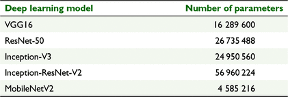
All the models were initialised with pre-trained weights trained on the ImageNet dataset. As the models were trained to recognise 1000 different objects, the original architecture was slightly modified to classify 20 crops and weed species. The last fully-connected layer of the original model was replaced by a global average pooling layer followed by two dense layers with 1024 neurones and ‘ReLU’ activation function. The output contained another dense layer where the number of neurons depended on the number of classes. The softmax activation function was used in the output layer since the models were multi-class classifiers. The size of the input was 256 × 256 × 3, and the batch size was 64. The maximum number of epochs for training the models was 100. However, often the training was completed before reaching the maximum number. The initial learning rate was set to 1 × 10⁻⁴ and is randomly decreased down to 10−6 by monitoring the validation loss in every epoch. Table 2 shows the number of parameters of each of the models used in this research without the output layer. It was found that the Inception-Resnet-V2 model has the most parameters, and the MobileNetV2 model has the least.
|
Transfer learning and fine-tuning
A conventional DL model contains two basic components: a feature extractor and a classifier. Depending on the DL model, different layers in the feature extractor and classifier may vary. However, all the DL architectures, used in this research, contain a series of trainable filters. Their weights are adjusted or trained for classifying images of a target dataset. Fig. 2a shows a basic structure of a pre-trained DL model. A pre-trained DL model means that the weights of the filters in the feature extractor and classifier is trained to classify 1000 different classes of images contained in the ImageNet dataset. The concept of TL is to use those pre-trained weights to classify the images of a new unseen dataset (Pan and Yang 2010; Guo et al. 2019). We used this approach in two different ways. The approaches were categorised as TL and FT. To train the model using our dataset of crop and weed images, we took the feature extractor from the pre-trained DL model and removed its classifier part since it was designed for a specific classification task. In the TL approach (Fig. 2b), we only trained the weights of the filters in the classifier part and kept the pre-trained weights of the layer in the feature extractor. This process eliminates the potential issue of training the complete network on a large number of labelled images. However, in the FT approach (Fig. 2c), the weights in the feature extractor were initialised from the pre-trained model, but not fixed. During the training phase of the model, the weights were retrained together with the classifier part. This process increased the efficiency of the classifier because it was not necessary to train the whole model from scratch. The model can extract discriminating features for the target dataset more accurately. Our experiments used both approaches and evaluated their performance on the crop and weed image dataset. Finally, we trained one state-of-the-art DL architecture from scratch, using our combined dataset (section 'Our combined dataset') and used its feature extractor to classify the images in an unseen test dataset (section 'Unseen test dataset') using the TL approach. The performance of the pre-trained state-of-the-art model was then compared with the model trained on the crop and weed dataset.

|
Performance metrics
The models were tested and thoroughly evaluated using several metrics: accuracy, precision, recall and F1 score metrics, which are defined as follows:
-
Accuracy (Acc): it is the percentage of images whose classes are predicted correctly among all the test images. A higher value represents a better result.
-
Precision (P): the fraction of correct prediction (True Positive) from the total number of relevant result (Sum of True Positives and False Positives).
-
Recall (R): the fraction of True Positive from the sum of True Positive and False Negative (number of incorrect predictions).
-
F1 Score (F1): the harmonic mean of precision and recall. This metric is useful to measure the performance of a model on a class-imbalanced dataset.
-
Confusion Matrix: it is used to measure the performance of machine learning models for classification problems. The confusion matrix tabulates the comparison of the actual target values with the values predicted by the trained model. It helps to visualise how well the classification model is performing and what prediction errors it is making.
In all these metrics, a higher value represents better performance.
Results and discussions
We conducted five sets of experiments on the data. Table 3 shows the number of images used for training, validation and testing of the models. Augmentation was applied to generate 4425 images for each of the classes. However, only actual images were used to validate and test the models. All the experiments were done on a desktop computer, with an Intel® Core™ i9-9900X processor, 128 gigabyte of RAM and a NVIDIA GeForce RTX 2080 Ti Graphics Processing Unit (GPU). We used the Professional Edition of the Windows 10 operating system. The deep learning models were developed using Python 3.8 and Tensorflow 2.4 framework.

|
Experiment 1: comparing the performance of DL models for classifying images in each of the datasets
In this experiment, we trained the five models separately on each dataset using only actual images (Table 3). Both TL and FT approaches were used to train the models. Table 4 shows the training, validation and testing accuracy for the five models.

|
On the ‘DeepWeeds’ dataset, the VGG16 model achieved the highest training, validation and testing accuracy (98.43%, 83.84% and 84.05%, respectively) using the TL approach. The training accuracy of the other four models was above 81%. However, the validation and testing accuracy for those models were less than 50%. This suggests that the models are overfitting. After FT the models, the overfitting problem was mitigated except for the MobileNetV2 architecture. Although four of the models achieved 100% training accuracy after FT, the validation and testing accuracy was between 86% and 94%. MobileNetV2 model still overfitted even after FT with about 32% validation and testing accuracy. Overall, the VGG16 model gave the best results for the ‘DeepWeeds’ dataset as they had the least convolutional layers, which was adequate for small datasets. It should be noted that Olsen et al. (2019), who initially worked on this dataset, achieved an average classification accuracy of 95.1% and 95.7% using Inception-V3 and ResNet-50, respectively. However, they applied data augmentation techniques to overcome the variable nature of the dataset.
On the ‘Corn Weed’ and ‘Cotton Tomato Weed’ datasets, the VGG16 and ResNet-50 models generally gave accurate result, but the accuracy of validation and testing were low for the DL models using the TL approach for both datasets, and the classification performance of the models was substantially improved after FT. Among the five models, the retrained Inception-ResNet-V2 model gave better results for the ‘Corn Weed’ dataset with training, validation and testing accuracy of 100%, 99.75% and 99.33% respectively. The ResNet-50 model accurately classified the images of the cotton tomato weed dataset.
VGG16 architecture reached about 99% classification accuracy on both validation and testing data of the ‘Soybean Weed’ dataset using the TL approach. Also, the performance of four other models are better for this dataset using pre-trained weights. Compared to other datasets, the ‘Soybean Weed’ dataset had more training samples, which helped to improve its classification performance. However, after FT the models on the datasets, all five deep learning architectures achieve more than 99% classification accuracy on the validation and testing data.
According to the results of this experiment, as shown in Table 4, it can be concluded that, for classifying the images of crop and weed species dataset, the TL approach does not work well. Since the pre-trained models were trained on the ‘ImageNet’ dataset (Deng et al. 2009), which does not contain images of crop or weed species, the models cannot accurately classify weed images.
Experiment 2: combining two datasets
In the previous experiment, we showed that it was unlikely to achieve better classification results using pre-trained weights for the convolutional layers of the DL models. The image classification accuracy improved by FT the weights of the models for the crop and weed dataset. For that reason, in this experiment, all the models were initialised with pre-trained weights and then retrained for the dataset. In this experiment, the datasets were paired up and used to generate six combinations to train the models. The training, validation and testing accuracies are shown in Table 5.

|
After FT the weights, all the DL models reached 100% training accuracy. The accuracy of the DL architectures also gave better validation and testing results when trained with CW-CTW, CW-SW, CTW-SW combined datasets. However, the models overfitted when trained on the ‘DeepWeeds’ dataset and combined with any of the other three datasets.
The results of the confusion matrix are provided in Fig. 3. We found that chinee apple, lantana, prickly acacia and snakeweed had a high confusion rate. This result agrees with that of Olsen et al. (2019). Visually, the images were quite similar and so were difficult to distinguish. That is why the DL model also failed to detect those. Since the dataset was small and did not have enough variations among the images, the models were not able to distinguish among the classes. The datasets also lacked enough images taken under different lighting conditions. The models were unable to detect the actual class of the images because of the illumination effects.

|
For the DW-CW dataset, the VGG16 model was more accurate. In this case, the model did not distinguish between chinee apple and snakeweed. As shown in the confusion matrix in Fig. 3a, 16 out of 224 test images of chinee apple were classified as snakeweed, and 23 of the 204 test images of snakeweed identified as chinee apple. A significant number of chinee apple and snakeweed images were not correctly predicted by the VGG16 model (see Fig. 3b). For the DW-SW dataset, the ResNet-50 model achieved 100% training, 97.68% validation and 97.42% testing accuracy. The confusion matrix is shown in Fig. 3c. The ResNet-50 model identified 13 chinee apple images as snakeweed, and the same number of snakeweed images were classified as chinee apple. The model also identified nine test images of snakeweed as lantana. Fig. 4 shows some sample images which the models classified incorrectly.

|
By applying data augmentation techniques, one can create more variations among the classes which may also help the model to learn more discriminating features.
Experiment 3: training the model with all four datasets together
In this experiment, all the datasets were combined to train the deep learning models. Classifying the images of the combined dataset is much more complex, as the data are highly class-imbalanced. The models were initialised with pre-trained weights and then fine-tuned. Table 6 shows the training, validation and testing accuracy and average precision, recall, and F1 scores achieved by the models on the test data.

|
After training the models with the combined dataset, the ResNet-50 model performed better. Though all the models except VGG16 achieved 100% training accuracy, the validation (97.83%) and testing (98.06%) accuracies of ResNet-50 architecture were higher. The average precision, recall and F1 score also verified these results. However, the models still did not correctly classify the chinee apple and snakeweed species mentioned in the previous experiment (Section Experiment 2: combining two datasets). A confusion matrix for predicting the classes of images using ResNet-50 is shown in Fig. 5. The confusion of ResNet-50 is chosen, since the highest accuracy is achieved in this experiment using this model. Seventeen chinee apple images were classified as snakeweed, and 15 snakeweeds images were classified incorrectly as chinee apple. In addition, the model also incorrectly classified some lantana and prickly acacia weed images. To overcome this classification problem, both actual and augmented data were used in the following experiment.

|
Experiment 4: training the models using both real and augmented images of the four datasets
Augmented data were used together with the real data in the training phase to address the misclassification problem in the previous experiment (section ‘Experiment 3: training the model with all four datasets together’). All the weed species and crop plant images had the same training data for this experiment. The models were initialised with pre-trained weights, and all the parameters were FT. Table 7 shows the result of this experiment.

|
From Table 7, we can see that the training accuracy for all the DL models is 100%. Also the validation and testing accuracies were reasonably high. In this experiment, the ResNet-50 models achieved the highest precision, recall and F1 score for the test data. Fig. 6 shows the confusion matrix for the ResNet-50 model. We compared the performance of the model using the confusion matrix with the previous experiment. The performance of the model was improved using both actual and augmented data. The classification accuracy increased for chinee apple, lantana, prickly acacia and snakeweed species by 2%.

|
In this research, the ResNet-50 model attained the highest accuracy using actual and augmented images. The Inception-ResNet-V2 model gave similar results. The explanation is that both of the models used residual layers. Residual connections help train a deeper neural network with better performance and reduced computational complexity. A deeper convolutional network works better when trained using a large dataset (Szegedy et al. 2017). Since we have used the augmented data and actual images, the dataset size has increased by several times.
Experiment 5: comparing the performance of two ResNet-50 models individually trained on ImageNet dataset, and the combined dataset, and testing on the unseen test dataset
In this experiment, we used two ResNet-50 models. The first was trained on our combined dataset with actual and augmented data (section ‘Our combined dataset’). Here, the top layers were removed from the model and a global average pooling layer and three dense layers were added as before. Other than the top layers, all the layers used pre-trained weights, which were not fine-tuned. This model termed as ‘CW ResNet-50’. The same arrangement was used for the pre-trained ResNet-50 model, which was instead trained on the ImageNet dataset. It was named as ‘SOTA ResNet-50’ model for further use. We trained the top layers of both models using the training split of the Unseen Test Dataset (2.1.6). Both models were tested using the test split of the Unseen Test Dataset. The confusion matrix for CW ResNet-50 and SOTA ResNet-50 model is shown in Fig. 7.

|
We can see in Fig. 7 that the performance of the two models is very similar. The ‘SOTA ResNet-50’ model detected all the classes of crop and weeds accurately. However, the pre-trained ‘CW Resnet-50’ model only identified two images incorrectly. As the ‘SOTA ResNet-50’ model was trained on a large dataset containing millions of images, it detected the discriminating features more accurately. In contrast, the ‘CW Resnet-50’ model was only trained on 88 500 images. If this model were trained with more data, it is probable that it would be more accurate using the TL approach. This type of pre-trained model could be used for classifying the images of new crop and weed datasets, which would eventually make the training process faster.
Conclusion
This study was undertaken on four image datasets of crop and weed species collected from four different geographical locations. The datasets contained a total of 20 different species of crops and weeds. We used five state-of-the-art CNN models, namely VGG16, ResNet-50, Inception-V3, Inception-ResNet-V2, MobileNetV2, to classify the images of these crops and weeds.
First, we evaluated the performance of TL and FT approaches of the models by training them on each dataset. The results showed that FT of the models could improve classification of the images more accurately than the TL approach.
To add more complexity to the classification problem, we combined the datasets together. After combining two of the datasets, the performance decreased due to some of the species of weeds in the ‘DeepWeeds’ dataset. The weed species that were confused were chinee apple, snakeweed, lantana and prickly acacia. We then combined all four datasets to train the models. Since the dataset was class-imbalanced, it was difficult to achieve high classification accuracy by only training the model with actual images. Consequently, we used augmentation to balance the classes of the dataset. However, it was evident that the models had problems in distinguishing between chinee apple and snakeweed. The performance of the models improved using both actual and augmented data. The models could distinguish chinee apple and snake weed more accurately. The results showed that the ResNet-50 was most accurate.
Another finding was that using the TL method was that in most cases the models did not achieve the desired accuracy. As ResNet-50 was the most accurate system, we ran a test using this pre-trained model. The model was used to classify the images of a new dataset using the TL approach. Although the model was not more accurate than the state-of-the-art pre-trained ResNet-50 model, it was very close to that. We could expect a higher accuracy using the TL approach if the model can be trained using a large crop and weed dataset.
This research shows that the data augmentation technique can help address the class imbalance problem and add more variations to the dataset. The variations in the images of the training dataset improve the training accuracy of the deep learning models. Moreover, the TL approach can mitigate the requirement of large data sets to train the deep learning models from scratch. The pre-trained models are trained on a large dataset to capture the detailed generalised features from the imagery, e.g. ImageNet in our case. However, because, ImageNet data set was not categorically labelled for weeds or crops, FT the pre-trained weights with crop and weed datasets help capture the dataset or task-specific features. Consequently, FT improves classification accuracy.
For training a DL model for classifying images, it is essential to have a large dataset like ImageNet (Deng et al. 2009) and MS-COCO (Lin et al. 2014). Classification of crop and weed species cannot be generalised unless a benchmark dataset is available. Most studies in this area are site-specific. A large dataset is needed to generalise the classification of crop and weed plants, and as an initial approach, large datasets can be generated by combining multiple small datasets, as demonstrated here. In this work, the images only had image-level labels. A benchmark dataset can be created by combining many datasets annotated with a variety of image labelling techniques. Generative Adversarial Networks (GANs) (Goodfellow et al. 2014) based image sample generation can also be used to mitigate class-imbalance issues. Moreover, it is needed to develop a crop and weed dataset annotated at the object level. For implementing a real-time selective herbicide sprayer, the classification of weed species is not enough. It is also necessary to locate the weeds in crops. DL-based object detection models can be used for detecting weeds.
Data availability
The data that support this study will be shared upon reasonable request to the corresponding author.
Conflicts of interest
The authors declare no conflicts of interest.
Declaration of funding
This research did not receive any specific funding.
References
Abadi M, Barham P, Chen J, et al. (2016) Tensorflow: a system for large-scale machine learning. In ‘Proceedings of the 12th USENIX symposium on operating systems design and implementation (OSDI ’16), 2–4 November 2016, Savannah, GA, USA’. pp. 265–283. (USENIX Association)Achanta R, Shaji A, Smith K, Lucchi A, Fua P, Süsstrunk S (2012) SLIC superpixels compared to state-of-the-art superpixel methods. IEEE Transactions on Pattern Analysis and Machine Intelligence 34, 2274–2282.
| SLIC superpixels compared to state-of-the-art superpixel methods.Crossref | GoogleScholarGoogle Scholar | 22641706PubMed |
Ahmad A, Saraswat D, Aggarwal V, Etienne A, Hancock B (2021) Performance of deep learning models for classifying and detecting common weeds in corn and soybean production systems. Computers and Electronics in Agriculture 184, 106081
| Performance of deep learning models for classifying and detecting common weeds in corn and soybean production systems.Crossref | GoogleScholarGoogle Scholar |
Ali-Gombe A, Elyan E (2019) MFC-Gan: class-imbalanced dataset classification using multiple fake class generative adversarial network. Neurocomputing 361, 212–221.
| MFC-Gan: class-imbalanced dataset classification using multiple fake class generative adversarial network.Crossref | GoogleScholarGoogle Scholar |
Chavan TR, Nandedkar AV (2018) AgroAVNET for crops and weeds classification: a step forward in automatic farming. Computers and Electronics in Agriculture 154, 361–372.
| AgroAVNET for crops and weeds classification: a step forward in automatic farming.Crossref | GoogleScholarGoogle Scholar |
Chollet F (2015) Keras. https://github.com/fchollet/keras
Dargan S, Kumar M, Ayyagari MR, Kumar G (2020) A survey of deep learning and its applications: a new paradigm to machine learning. Archives of Computational Methods in Engineering 27, 1071–1092.
| A survey of deep learning and its applications: a new paradigm to machine learning.Crossref | GoogleScholarGoogle Scholar |
Deng J, Dong W, Socher R, Li L-J, Li K, Fei-Fei L (2009) Imagenet: a large-scale hierarchical image database. In ‘2009 IEEE conference on computer vision and pattern recognition’. pp. 248–255. (IEEE)
| Crossref |
Dyrmann M, Karstoft H, Midtiby HS (2016) Plant species classification using deep convolutional neural network. Biosystems Engineering 151, 72–80.
| Plant species classification using deep convolutional neural network.Crossref | GoogleScholarGoogle Scholar |
Espejo-Garcia B, Mylonas N, Athanasakos L, Fountas S, Vasilakoglou I (2020) Towards weeds identification assistance through transfer learning. Computers and Electronics in Agriculture 171, 105306
| Towards weeds identification assistance through transfer learning.Crossref | GoogleScholarGoogle Scholar |
Ferreira AdS, Freitas DM, da Silva GG, Pistori H, Folhes MT (2017) Weed detection in soybean crops using convnets. Computers and Electronics in Agriculture 143, 314–324.
| Weed detection in soybean crops using convnets.Crossref | GoogleScholarGoogle Scholar |
Gando G, Yamada T, Sato H, Oyama S, Kurihara M (2016) Fine-tuning deep convolutional neural networks for distinguishing illustrations from photographs. Expert Systems with Applications 66, 295–301.
| Fine-tuning deep convolutional neural networks for distinguishing illustrations from photographs.Crossref | GoogleScholarGoogle Scholar |
Girshick R, Donahue J, Darrell T, Malik J (2014) Rich feature hierarchies for accurate object detection and semantic segmentation. In ‘Proceedings of the IEEE conference on computer vision and pattern recognition’. pp. 580–587.
Goodfellow I, Pouget-Abadie J, Mirza M, Xu B, Warde-Farley D, Ozair S, Courville A, Bengio Y (2014) Generative adversarial networks. Advances in neural information processing systems, 27.
Guo Y, Shi H, Kumar A, Grauman K, Rosing T, Feris R (2019) Spottune: transfer learning through adaptive fine-tuning. In ‘Proceedings of the IEEE/CVF conference on computer vision and pattern recognition’. pp. 4805–4814. (IEEE)
Harker KN, O’Donovan JT (2013) Recent weed control, weed management, and integrated weed management. Weed Technology 27, 1–11.
| Recent weed control, weed management, and integrated weed management.Crossref | GoogleScholarGoogle Scholar |
Hasan AMMM, Sohel F, Diepeveen D, Laga H, Jones MGK (2021) A survey of deep learning techniques for weed detection from images. Computers and Electronics in Agriculture 184, 106067
| A survey of deep learning techniques for weed detection from images.Crossref | GoogleScholarGoogle Scholar |
He K, Zhang X, Ren S, Sun J (2016) Deep residual learning for image recognition. In ‘Proceedings of the IEEE conference on computer vision and pattern recognition’. pp. 770–778. (IEEE)
Hentschel C, Wiradarma TP, Sack H (2016) Fine tuning cnns with scarce training data – adapting imagenet to art epoch classification. In ‘2016 IEEE international conference on image processing (ICIP)’. pp. 3693–3697. (IEEE)
| Crossref |
Iqbal N, Manalil S, Chauhan BS, Adkins SW (2019) Investigation of alternate herbicides for effective weed management in glyphosate-tolerant cotton. Archives of Agronomy and Soil Science 65, 1885–1899.
| Investigation of alternate herbicides for effective weed management in glyphosate-tolerant cotton.Crossref | GoogleScholarGoogle Scholar |
Jensen TA, Smith B, Defeo LF (2020) An automated site-specific fallow weed management system using unmanned aerial vehicles. Paper presented at the GRDC Grains Research Update in Goondiwindi, Qld.
Jiang H, Zhang C, Qiao Y, Zhang Z, Zhang W, Song C (2020) CNN feature based graph convolutional network for weed and crop recognition in smart farming. Computers and Electronics in Agriculture 174, 105450
| CNN feature based graph convolutional network for weed and crop recognition in smart farming.Crossref | GoogleScholarGoogle Scholar |
Kamilaris A, Prenafeta-Boldú FX (2018) Deep learning in agriculture: a survey. Computers and Electronics in Agriculture 147, 70–90.
| Deep learning in agriculture: a survey.Crossref | GoogleScholarGoogle Scholar |
Khan SH, Hayat M, Bennamoun M, Sohel FA, Togneri R (2017) Cost-sensitive learning of deep feature representations from imbalanced data. IEEE Transactions on Neural Networks and Learning Systems 29, 3573–3587.
| Cost-sensitive learning of deep feature representations from imbalanced data.Crossref | GoogleScholarGoogle Scholar | 28829320PubMed |
Krawczyk B (2016) Learning from imbalanced data: open challenges and future directions. Progress in Artificial Intelligence 5, 221–232.
| Learning from imbalanced data: open challenges and future directions.Crossref | GoogleScholarGoogle Scholar |
Lameski P, Zdravevski E, Trajkovik V, Kulakov A (2017) Weed detection dataset with rgb images taken under variable light conditions. In ‘ICT Innovations 2017’. Communications in computer and information science. (Eds D Trajanov, V Bakeva) pp. 112–119 (Springer: Cham, Switzerland)
Lameski P, Zdravevski E, Kulakov A (2018) Review of automated weed control approaches: an environmental impact perspective. In ‘Proceedings of the 10th International Conference’. ICT Innovations 2018, 17–19 September 2018, Ohrid, Macedonia. pp. 132–147. (Springer)
Lin T-Y, Maire M, Belongie S, Hays J, Perona P, Ramanan D, Dolla’r P, Zitnick CL (2014). Microsoft coco: common objects in context. In ‘Computer Vision – ECCV 2014. ECCV 2014’. Lecture notes in computer science. vol. 8693. (Eds D Fleet, T Pajdla, B Schiele, T Tuytelaars) pp. 740–755. (Springer: Cham, Switzerland)
López-Granados F (2011) Weed detection for site-specific weed management: mapping and real-time approaches. Weed Research 51, 1–11.
| Weed detection for site-specific weed management: mapping and real-time approaches.Crossref | GoogleScholarGoogle Scholar |
McLeod R (2018) Annual costs of weeds in australia. Available at https://invasives.com.au/wp-content/uploads/2019/01/Cost-of-weeds-report.pdf
Medina-Pastor P, Triacchini G (2020) The 2018 european union report on pesticide residues in food. EFSA Journal 18, e06057
Nkemelu DK, Omeiza D, Lubalo N (2018) Deep convolutional neural network for plant seedlings classification. arXiv preprint arXiv:1811.08404.
Olsen A, Konovalov DA, Philippa B, et al. (2019) Deepweeds: a multiclass weed species image dataset for deep learning. Scientific Reports 9, 1–12.
Pan SJ, Yang Q (2010) A survey on transfer learning. IEEE Transactions on Knowledge and Data Engineering 22, 1345–1359.
| A survey on transfer learning.Crossref | GoogleScholarGoogle Scholar |
Peteinatos G, Reichel P, Karouta J, Andújar D, Gerhards R (2020) Weed identification in maize, sunflower, and potatoes with the aid of convolutional neural networks. Remote Sensing 12, 4185
| Weed identification in maize, sunflower, and potatoes with the aid of convolutional neural networks.Crossref | GoogleScholarGoogle Scholar |
Robocrop spot sprayer: weed removal (2018) Available at https://garford.com/products/robocrop-spot-sprayer/. [Retrieved January 25, 2021]
Sabottke CF, Spieler BM (2020) The effect of image resolution on deep learning in radiography. Radiology: Artificial Intelligence 2, e190015
| The effect of image resolution on deep learning in radiography.Crossref | GoogleScholarGoogle Scholar | 33937810PubMed |
Sahlsten J, Jaskari J, Kivinen J, Turunen L, Jaanio E, Hietala K, Kaski K (2019) Deep learning fundus image analysis for diabetic retinopathy and macular edema grading. Scientific Reports 9, 10750
| Deep learning fundus image analysis for diabetic retinopathy and macular edema grading.Crossref | GoogleScholarGoogle Scholar | 31341220PubMed |
Sandler M, Howard A, Zhu M, Zhmoginov A, Chen L-C (2018) Mobilenetv2: inverted residuals and linear bottlenecks. In ‘Proceedings of the IEEE conference on computer vision and pattern recognition’. pp. 4510–4520. (IEEE)
Shao L, Zhu F, Li X (2015) Transfer learning for visual categorization: a survey. IEEE Transactions on Neural Networks and Learning Systems 26, 1019–1034.
| Transfer learning for visual categorization: a survey.Crossref | GoogleScholarGoogle Scholar | 25014970PubMed |
Simonyan K, Zisserman A (2014) Very deep convolutional networks for large-scale image recognition. In ‘International conference on learning representations (ICLR)’. 7–9 May 2015, San Diego, CA, USA. (ICLR).
Slaughter DC, Giles DK, Downey D (2008) Autonomous robotic weed control systems: a review. Computers and Electronics in Agriculture 61, 63–78.
| Autonomous robotic weed control systems: a review.Crossref | GoogleScholarGoogle Scholar |
Steinberg R (2017) 6 areas where artificial neural networks outperform humans. Available at https://venturebeat.com/2017/12/08/6-areas-where-artificial-neural-networks-outperform-humans/ [Accessed 25 December 2020]
Suh HK, Ijsselmuiden J, Hofstee JW, van Henten EJ (2018) Transfer learning for the classification of sugar beet and volunteer potato under field conditions. Biosystems Engineering 174, 50–65.
| Transfer learning for the classification of sugar beet and volunteer potato under field conditions.Crossref | GoogleScholarGoogle Scholar |
Szegedy C, Vanhoucke V, Ioffe S, Shlens J, Wojna Z (2016) Rethinking the inception architecture for computer vision. In ‘Proceedings of the IEEE conference on computer vision and pattern recognition’. pp. 2818–2826. (IEEE)
Szegedy C, Ioffe S, Vanhoucke V, Alemi A (2017) Inception-v4, inception-resnet and the impact of residual connections on learning. In ‘Proceedings of the AAAI conference on artificial intelligence’. 31(1). (AAAI Press)
Teimouri N, Dyrmann M, Nielsen PR, Mathiassen SK, Somerville GJ, Jørgensen RN (2018) Weed growth stage estimator using deep convolutional neural networks. Sensors 18, 1580
| Weed growth stage estimator using deep convolutional neural networks.Crossref | GoogleScholarGoogle Scholar |
Tian H, Wang T, Liu Y, Qiao X, Li Y (2020) Computer vision technology in agricultural automation—a review. Information Processing in Agriculture 7, 1–19.
| Computer vision technology in agricultural automation—a review.Crossref | GoogleScholarGoogle Scholar |
Van der Walt S, Schönberger JL, Nunez-Iglesias J, Boulogne F, Warner JD, Yager N, Gouillart E, Yu T (2014) Scikit-image: image processing in python. PeerJ 2, e453
| Scikit-image: image processing in python.Crossref | GoogleScholarGoogle Scholar | 25024921PubMed |
Wäldchen J, Mäder P (2018) Plant species identification using computer vision techniques: a systematic literature review. Archives of Computational Methods in Engineering 25, 507–543.
| Plant species identification using computer vision techniques: a systematic literature review.Crossref | GoogleScholarGoogle Scholar | 29962832PubMed |
Weedseeker 2 spot spray system (n.d.) Available at https://agriculture.trimble.com/product/weedseeker-2-spot-spray-system/ [Accessed 25 January 2021]