

Initialising reservoir models for history matching using pre-production 3D seismic data: constraining methods and uncertainties
Mohammad Emami Niri 1 3 David E. Lumley 1 21 School of Earth and Environment, University of Western Australia, 35 Stirling Highway, Crawley, WA 6009, Australia.
2 School of Physics, University of Western Australia, 35 Stirling Highway, Crawley, WA 6009, Australia.
3 Corresponding author. Email: mohammad1199@gmail.com
Exploration Geophysics 48(1) 37-48 https://doi.org/10.1071/EG15013
Submitted: 14 February 2015 Accepted: 30 August 2015 Published: 1 October 2015
Abstract
Integration of 3D and time-lapse 4D seismic data into reservoir modelling and history matching processes poses a significant challenge due to the frequent mismatch between the initial reservoir model, the true reservoir geology, and the pre-production (baseline) seismic data. A fundamental step of a reservoir characterisation and performance study is the preconditioning of the initial reservoir model to equally honour both the geological knowledge and seismic data. In this paper we analyse the issues that have a significant impact on the (mis)match of the initial reservoir model with well logs and inverted 3D seismic data. These issues include the constraining methods for reservoir lithofacies modelling, the sensitivity of the results to the presence of realistic resolution and noise in the seismic data, the geostatistical modelling parameters, and the uncertainties associated with quantitative incorporation of inverted seismic data in reservoir lithofacies modelling. We demonstrate that in a geostatistical lithofacies simulation process, seismic constraining methods based on seismic litho-probability curves and seismic litho-probability cubes yield the best match to the reference model, even when realistic resolution and noise is included in the dataset. In addition, our analyses show that quantitative incorporation of inverted 3D seismic data in static reservoir modelling carries a range of uncertainties and should be cautiously applied in order to minimise the risk of misinterpretation. These uncertainties are due to the limited vertical resolution of the seismic data compared to the scale of the geological heterogeneities, the fundamental instability of the inverse problem, and the non-unique elastic properties of different lithofacies types.
Key words: 3D and time-lapse 4D seismic, elastic properties, geostatistics, lithofacies modelling, seismic inversion, uncertainty analysis.
Introduction
A depositional facies (herein simply referred to as ‘facies’) is a distinctive body of rock that forms under specific conditions of sedimentation and hence has particular characteristics (Reading, 2009). This conceptual definition highlights that it is important to include facies modelling as a key part of static and dynamic reservoir studies. Porosity, permeability, clay content, degree of heterogeneity and connectivity are often simulated on the basis of facies distribution, and the distribution of facies mainly depends on the geological processes (Saussus and Sams, 2012; Pyrcz and Deutsch, 2014). Geological knowledge about a given reservoir is always incomplete, because of limited well coverage and complex subsurface heterogeneity (Dutton et al., 2003; Eaton, 2006). In this context, 3D seismic data, due to its high spatial density, plays a critical role — not only by defining the reservoir structure and geometry, but also in constraining the reservoir property variations (Doyen, 2007). To produce realistic models of the reservoir facies and corresponding petrophysical properties, and to avoid biased or non-physical results, seismic-related information should be simultaneously incorporated with all other available static and dynamic data in the model-building process. This can be achieved, for example, by using geostatistical simulation techniques (e.g. Deutsch and Journel, 1992; Araktingi and Bashore, 1992; Behrens et al., 1998; Caers et al., 2001; Mukerji et al., 2001; Dubrule, 2003).
Geostatistical reservoir modelling has become standard practice in the energy industry, and is widely used for hydrocarbon reserve estimation, targeting new producer/injector locations, and production profile forecasting with flow simulators (Caers, 2005; Zakrevsky, 2011). Static reservoir models are typically built using time-independent static reservoir data that has been measured once in time, including well logs, core measurements and pre-production 3D seismic surveys. These models are then updated in a history matching process to be consistent with dynamic reservoir data during the production phase (e.g. historical production data and/or time-lapse 4D seismic data). Reservoir history matching is a highly underdetermined and nonlinear inverse problem, and is therefore very sensitive to the initial starting model. In particular, when including 4D seismic data in the reservoir history matching process, it is essential that the synthetic 3D seismic data modelled from the initial static reservoir model closely matches the real baseline 3D seismic data. Without this initial match, the use of subsequent 4D seismic datasets to update reservoir simulation models introduces considerable uncertainty and risk (Lumley and Behrens, 1998; Da Veiga and Le Ravalec-Dupin, 2010; Le Ravalec-Dupin et al., 2011).
Despite the fact that seismic data is an excellent source of information beyond the wells, seismic reflection amplitudes do not often give a direct interpretation of reservoir lithofacies and petrophysical properties (e.g. Bornard et al., 2005). In this context, seismic inversion is conventionally used to transform seismic reflection amplitudes into subsurface elastic properties (e.g. velocities and impedances). The scope of seismic reservoir characterisation, however, goes beyond simply inverting the seismic data to obtain the elastic parameters of the rock, and attempts to obtain the reservoir properties such as lithofacies and porosity from the seismic data; This may be performed (1) by using a sequential or multistep scheme (seismic inversion followed by estimation of reservoir properties from the seismic-inverted data), or (2) based on a unified inversion scheme (direct petrophysical inversion of seismic reflection amplitudes) (Kemper, 2010; Bosch et al., 2010; Grana et al., 2012). A common approach in reservoir lithofacies and petrophysical property modelling is the quantitative incorporation of various seismic elastic properties (e.g. inverted P- and S-impedances) as sources of additional information to guide/constrain geostatistical interpolation of reservoir properties away from the wells, thus producing multiple equi-probable realisations of reservoir properties to account for uncertainties and spatial variations. Many successful applications of this approach have been reported in the literature (Doyen, 1988; Rossini et al., 1994; Nivlet et al., 2005; Delfiner and Haas, 2005); however, the associated technical obstacles, such as the difference in scale at which measurements are made and the low-frequency content of the seismic data, can lead to biased or non-physical results (Francis, 2010; Saussus and Sams, 2012).
In this paper we investigate issues that have impact on the match of the initial reservoir model with well logs and inverted 3D seismic data. Specifically, we address the following questions:
-
Which of the common constraining methods in variogram-based lithofacies modelling produces reservoir models that best match the inverted 3D seismic data?
-
How are the results affected by the presence of noise in the observed data, and by the low vertical resolution of seismic data compared to scale of the geological heterogeneities?
-
What is the effect of uncertain geostatistical variogram parameters on the results?
-
What are the uncertainties and limitations in quantitatively incorporating deterministic seismic inversion results in reservoir lithofacies modelling?
The remainder of this paper is organised in three main sections. The second section provides an overview of the test model construction. In the third section, we describe our constraining methods applied in the reservoir lithofacies modelling process, followed by a discussion of the modelling results and the sensitivities to noise and variogram parameters. Finally, in the last section, we analyse the uncertainties in the quantitative incorporation of inverted 3D seismic data in reservoir lithofacies modelling, followed by a discussion of these uncertainties in which we address seismic resolution limitations and overlapping elastic properties of different lithofacies types.
Test model
We construct a synthetic dataset (for simplicity, two lithology types and one elastic property) to act as a basis for analysing seismic constraining methods in geostatistical lithofacies modelling, and also for investigating the sensitivity of the results to (1) noise in the seismic data, and (2) differences in the parameters of the geostatistical variogram.
We first construct a base reservoir lithofacies model, consisting of clean sand and shaly sand. The model covers an area of 6 km2 and the reservoir gross thickness is 100 m. Pure shale units, also 100 m thick, form the upper and lower boundaries. This 3D model contains 212 × 184 × 140 grid blocks with dimensions 12.5 × 12.5 × 1 m3. The clean sand and shaly sand distributions within the reservoir interval are modelled using the sequential indicator simulation (SIS) technique (Journel and Gomez-Hernandez, 1993), with an exponential variogram range of 20 m in the vertical direction and 1000 m in the major and minor horizontal directions for both the clean sand and the shaly sand. The thickness of the clean sand bodies range from values less than seismic resolution to greater than seismic resolution. The lithofacies model generated in this way (Figure 1a) is assumed to be the true (reference) model. The small net-to-gross value (~20%) addresses the prediction uncertainties in zones of small net sand thickness. Seven well trajectories are then constructed at predefined positions within the reservoir framework, and the blocked litho-logs are obtained by identifying the grid blocks intersecting the well trajectories. Within each facies, the porosity distribution is found using the sequential Gaussian simulation (SGS) technique (Deutsch and Journel, 1992) from an exponential variogram with a vertical range of 10 m and horizontal range of 500 m in the principal directions.
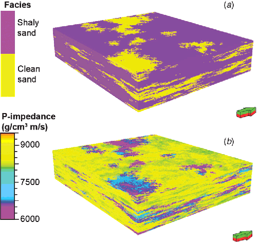
|
We use a petro-elastic model to compute the P-wave impedance volume for the reference lithofacies model, based on theoretical and experimental relationships (Appendix A). The elastic properties of the clean sand and shaly sand in the reservoir at initial conditions are given in Table 1. In addition, we assume a two-phase fluid (oil and water) to be present in the pore system; the fluid properties are given in Table 2. For the sake of simplicity, the oil–water contact is assumed to be flat (constant) in depth, with a constant distribution of the fluids within each of the fluid layers. Water saturation below the oil–water contact is assumed to be equal to 1. Above the contact it is equal to the irreducible water saturation value (0.2 for clean sand; 0.7 for shaly sand); however, it is possible to simulate the irreducible water saturation using a geostatistical technique (e.g. SGS) or by flow simulation to improve the realism of the model. For testing purposes, we assume the computed P-wave impedance volume (Figure 1b) to be the reference (true) impedance volume that would result from a perfect inversion of the baseline seismic survey. It is worth noting that due to the bandlimited nature of seismic data, inverting the data accurately to the resolution of model (1 m vertical cells in this case) is unrealistic and would not be possible in real world applications.

|
|
The petro-elastic model gives a reasonable approximation of the elastic properties of rocks, but it cannot perfectly represent the real heterogeneities of the subsurface rocks. To increase the realism of the test model, and also to examine the robustness of the constraining methods in the presence of noise and limited resolution in the inverted seismic data, following noise-variation options are considered:
-
Noise0: Noise-free P-impedance volume.
-
Noise1: Up to 20% bandlimited (10–60 Hz) random noise added to the P-impedance values along all three directions.
-
Noise2: To simulate the limited frequency range of the deterministic seismic inversion results and the low vertical resolution of seismic data compared to the scale of the reservoir model, we apply a moving-average smoothing filter to the impedance volumes, replacing the data in each cell of the 3D grid with the average of the data in neighbouring cells (2 cells in lateral directions and 5 cells in vertical direction). This means that the resolution of the P-impedance volume for Noise2 conditions decreases from 12.5 × 12.5 × 1 m3 to 25 × 25 × 5 m3. This is equivalent to low-pass frequency-wavenumber filtering of the 3D impedance volume with an assumption that low frequencies have been reasonably recovered in the inversion process by constraining to well data.
-
Noise3: To approximate a more realistic scenario, a combination of Noise1 and Noise2 conditions are added to the high resolution P-impedance volume (i.e. Noise3 ~ Noise1 + Noise2).
To analyse how seismic amplitudes change for different noise and resolution conditions we have computed synthetic seismic traces; for each noise scenario the corresponding P-impedance model is used to compute P-wave reflection coefficients, which are then convolved with a 30 Hz Ricker wavelet to generate zero-offset seismic traces. Figure 2a–d shows the seismic amplitude maps at the top of the reservoir for all four noise scenarios (Noise0, Noise1, Noise 2 and Noise3). The effects of each noise scenario are clearly visible on the seismic amplitude maps.

|
It is possible to invert the synthetic seismic data using a common post-stack seismic inversion scheme such as recursive inversion (Lindseth, 1979), sparse-spike inversion (e.g. Oldenburg et al., 1983), model-based inversion (Russell and Hampson, 1991) or coloured inversion (Lancaster and Whitcombe, 2000) to produce inverted P-impedance models for each of the noise scenarios. However, each of these seismic inversion algorithms has its own limitations and shortcomings (e.g. Sen, 2006). In our test case study, given the objectives of this paper, and to avoid the specific limitations and errors caused by the chosen seismic inversion algorithm, we assume that the introduced noise conditions to the high resolution P-impedance volume reasonably represent the inverted P-impedance models. However, in real data case studies, issues such as wavelet estimation, construction of low frequency background model, etc. are of great importance to achieve reliable seismic inversion results.
Constraining methods in geostatistical lithofacies modelling
To construct reservoir lithofacies models using a geostatistical simulation technique, we employ four constraining methods in addition to the estimated variogram parameters from litho-logs. In method 1, we define an additional constraint from well log information. In methods 2, 3 and 4, we include P-impedance volume as an extra dimension to generate seismically-constrained lithofacies models.
Method 1: vertical probability curves of litho-logs
In this method, well data without knowledge of the seismic attributes is considered. Based on the litho-logs from seven wells (in our test model application), we generate the vertical probability curves (e.g. blue curve in Figure 3) that determine the proportions of clean sand and shaly sand in each layer of the reservoir interval. For example, in layer 1 one of the wells encountered clean sand and the other six wells encountered shaly sand. This implies that in layer 1 the probability of occurrence of clean sand and shaly sand are 15% and 85%, respectively. We repeat this process for all layers in the reservoir interval to generate the vertical probability curves of clean sand and shaly sand. We then use these proportions as an extra constraint, along with variogram parameters, to populate the facies indicators in the entire 3D framework of the reservoir. Since seismic data is not incorporated in this process, the probability curve is identical for all noise varying options (Noise0, Noise1, Noise2 and Noise3). It is worth noting that this method works under the assumption that the available well data represents a good approximation of the true facies proportions for each layer. Naturally, more wells would provide more accuracy in the estimation of correct vertical litho-probability curves. In addition, the presence of geologic structure in the subsurface can add more uncertainty in the estimated curves; therefore, it is recommended to use this method along with other data such as seismic amplitude maps to help constrain the process of lithofacies modelling.
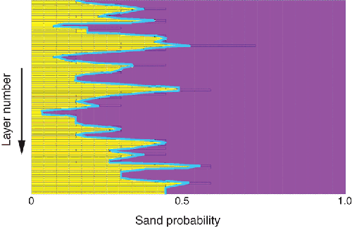
|
Method 2: seismic attribute litho-probability curves
In this method, the probability of facies distribution is obtained as a function of a seismic attribute property. We first analyse the relationship between lithofacies indicators and values of various seismic attribute properties at well locations to determine the most suitable link between seismic and geological properties. We then plot the probability density distributions, relating the selected seismic elastic property (P-wave impedance, in our test case) to the probability of each lithofacies type. The plot gives the probability of finding a particular lithofacies given a specific range of P-wave impedance values. This analysis produces a probability curve for each of the lithofacies types (e.g. blue curve in Figure 4 for clean sand) that gives the constraint values. We then use the generated seismic litho-probability curves, along with variogram parameters, to guide the process of lithofacies modelling in a geostatistical simulation technique. It may be readily understood that noise in the seismic data attributes (P-wave impedance, in our test case) will affect this process and that the extracted litho-probability curves, and therefore the constraint values will be different for the Noise0, Noise1, Noise2 and Noise3 conditions.
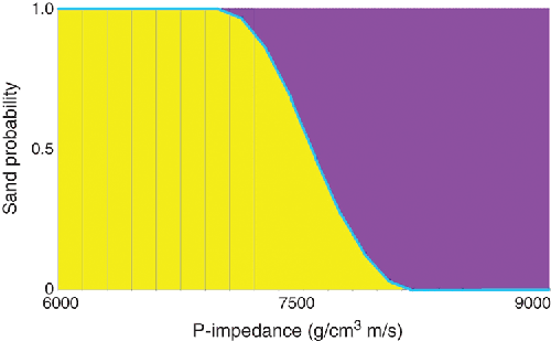
|
Method 3: seismic attribute litho-probability cubes
To generate seismic litho-probability cubes, we extract probability density functions, relating seismic elastic attributes to the probability of each lithofacies type. We then apply the derived functions in a Bayesian framework to the P-wave impedance volume to model 3D probability cubes for each particular lithofacies type. In general, Bayes decision theory is a well known approach for probabilistic classification problems (Duda et al., 2001). In the energy industry it has become a widely used approach for describing the particular reservoir static or dynamic class or state that is of interest, such as lithofacies, saturation, pressure and so on (e.g. Mukerji et al., 2001; Coléou et al., 2006; Nivlet et al., 2007). Bayesian formulation is adapted to the present problem for calculating the posterior probability of each particular lithofacies, given a set of seismic attributes (Avseth et al., 2005):

where f is a lithofacies type; A is a vector of the seismic attribute; p(f) is a prior probability of lithofacies f; p(A) is the probability of seismic attribute A; p(A|f) is the probability of attribute A given the lithofacies f; and p(f|A) is the probability of lithofacies f given the seismic attribute vector A.
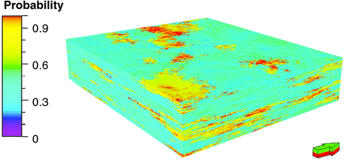
In the test application there are two lithofacies types (f = {clean sand, shaly sand}) and one seismic elastic attribute(A = {Ip}); therefore we generate two seismic litho-probability cubes — one for clean sand (Figure 5) and one for shaly sand. These cubes represent the probability of each lithofacies at the seismic scale. We then use the litho-probability volumes, along with variogram parameters, to guide the process of lithofacies modelling in a geostatistical simulation technique. Clearly, the modelled litho-probability cubes are different for each noise-variation option.
|
Method 4: seismic attribute litho-probability surfaces
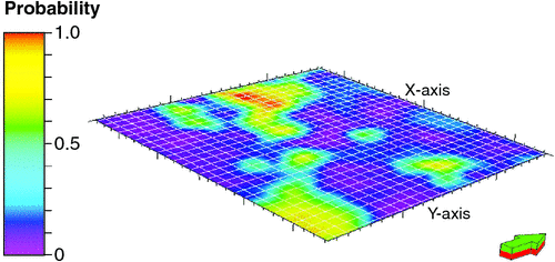
In this method, the areal probability of facies distribution is given by the seismic attribute trend surfaces. We first analyse the relationship between lithofacies indicators and values of the selected seismic property (P-impedance in our test case) at well locations to determine the link between seismic and facies indicators. We then extract a surface map of the P-wave impedance at the top of the reservoir; this map is similar (but not identical) to the commonly-used seismic amplitude map at the top of the reservoir. We then normalise the P-wave impedance surface to extract the litho-probability trend surface (Figure 6). We use the seismic attribute litho-probability surfaces as 2D areal constraints together with the vertical probability curves of the litho-logs (introduced in method 1) as 1D vertical trends, in addition to variogram parameters, to guide the 3D lithofacies simulation process. As in constraining methods 2 and 3, the extracted seismic attribute trend surface is different for each of the noise-variation options.
|
Lithofacies modelling results
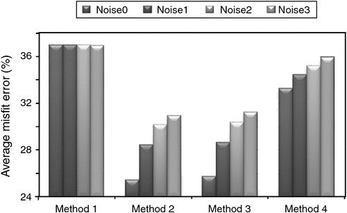
This section sets out a quantitative comparison of the lithofacies modelling results in terms of the average misfit error between the simulated models and the true reference model. When a true model is available, the average misfit error is a useful tool for quantifying the performance of the prediction in supervised learning. After calculating the misfit error of each individual model from the number of grid-blocks whose assigned lithofacies indicators differ from the corresponding grid-blocks in the true model, we calculate the average misfit error for twenty realisations. We repeat this process for all the four constraining methods and the four noise varying options. The bar graph in Figure 7 summarises the results.
|
Figure 7 shows that method 1 gives the highest average misfit error for all noise options; by contrast, methods 2 and 3 yield the least misfit error with the best match to the reference model. The average misfit error of the simulated models using constraining method 4 is greater than for methods 2 and 3, but is less than for method 1. The analyses also demonstrate that, although the presence of noise in the observed data increases the average misfit errors, incorporating P-impedance volume into the reservoir model nevertheless improves the match, with methods 2 and 3 giving the best results. It is also evident that error caused by the limited resolution of the P-impedance volume produces a more adverse effect than added random noise. For instance, in method 2, the average misfit error increases from around 25.5% (Noise0) to more than 28.5% in Noise1 and 30% in Noise2. In addition, the analyses show that presence of a combination of Noise1 and Noise2 (= Noise3) in the P-impedance volume results in the highest misfit error for all seismic constraining methods.
The question arises about why constraining methods 2 and 3 simulate models with the least misfit error to the true reference model. This is because of the fact that methods 2 and 3 provide a natural way of incorporating inverted seismic data for 3D lithofacies simulation. Using these constraining methods we can define 3D seismic constraints more accurately (not only 1D vertical constraint as in method 1 or 2D areal constraint as in method 4) that can be easily incorporated in pixel-based lithofacies simulation process. It is also notable that although constraining method 2 gives similar misfit errors to method 3 in this test application, it should be cautiously applied especially in areas with fewer wells (fewer control points), such that there is not enough confidence to generate an accurate seismic attribute litho-probability curve. On the other hand, when there are more than two lithofacies types within the reservoir interval of interest or when the pre-stack seismic inversion (e.g. simultaneous elastic inversion (Fatti et al., 1994; Hampson et al., 2005)) has produced several seismic elastic properties such as P-impedance, S-impedance and density, method 3 might define the constraint more accurately in lithofacies modelling. This can be performed by the use of a combination of several seismic elastic properties to generate multivariate probability density functions for reducing ambiguity in Bayesian classification of each particular lithofacies type (e.g. Avseth et al., 2005). An example of a successful application of constraining method 3 (i.e. the Bayesian classification technique) using multiple seismic-inverted elastic attributes (P-impedance, Vp/Vs ratio and density) for reservoir property modelling for a real data case study from offshore Western Australia is presented by Emami Niri and Lumley (2014). In addition, an application of the constraining method 2 in a real data case study to generate starting reservoir model for a subsequent multi-objective reservoir modelling process is discussed in Emami Niri and Lumley (2015).
Thus far in the analyses, we have used an exponential variogram model (Equation 2) estimated from upscaled litho-logs, where the lateral and vertical ranges are defined as the separation distance at which the variogram model reaches 0.95 of its sill (Isaaks and Srivastava, 1989):

where c = sill – nugget (in our case nugget = 0.2 and sill = 1); h = 0.95c; and R is the variogram range. The major and minor horizontal ranges are specified to be ~1000 m; and the vertical range is specified to be ~20 m.
To study the effect of uncertain variogram parameters on the reservoir lithofacies modelling result, we consider the following variations:
-
Analysis 1: Long distances for variogram ranges
-
Analysis 2: Variogram ranges estimated from well logs
-
Analysis 3: Short distances for variogram ranges.
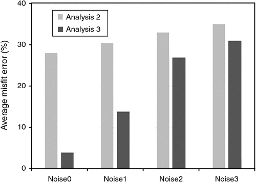
Figure 8 shows the sensitivity of the geostatistical lithofacies modelling process to variogram parameters for constraining method 2. It is evident that higher variogram ranges yields unreasonable models, since they do not agree with either the well log data or the seismic attributes; however smaller variogram ranges result in the best match. This is mainly due to the fact that, by using short distances for variogram ranges, the input seismic constraint (the seismic attribute litho-probability curve, in this case) is fully respected — in other words, the extent of the heterogeneities of the reservoir lithofacies is no longer linked to the variogram, but rather it is largely controlled by the seismic constraint. This implies that small variogram ranges should be used only when the quality of the inverted seismic data is highly reliable since, as illustrated in Figure 8, the misfit error rises considerably from Noise0 to Noise1, Noise 2 and Noise3.
|
Figure 9 shows that there is an excellent qualitative match between the true reference lithofacies model and a realisation of the simulated models using short variogram ranges and constrained by method 2 in Noise0 option. According to analysis 3 of Noise0 option in Figure 8, the average misfit error between these two models is just 3%. It is notable that the excellent match between true and seismic-constrained models is an idealised situation that rarely obtainable in real cases. This is because of the fact that noise in the observed seismic data together with fundamental insatiability of seismic inverse problems results in the lack of confidence to use very short variogram ranges (to fully respect the input seismic constraint).

|
Uncertainty analysis
It is common practice to incorporate 3D seismic information in reservoir lithofacies and petrophysical property modelling; however, the associated limits and uncertainties need to be clarified in order to minimise the risk of misinterpretation. This section describes an analysis of the uncertainties arising when deterministic seismic inversion results are incorporated in reservoir lithofacies modelling. These uncertainties are due to (1) limited seismic resolution compared to the scale of the geological heterogeneities, and (2) the non-unique elastic properties of the different lithofacies types.
To analyse uncertainties, we use a similar approach to the one presented by Sams and Saussus (2010). For the same base lithofacies model, we generate several P-impedance volumes using the SGS technique with an exponential variogram range of 10 m vertically and 1000 m in the major and minor horizontal directions. We generate different impedance volumes to have various degrees of overlapping P-impedance properties for clean sand and shaly sand. The means of the distributions for all P-impedance models are assigned as constant values: 6500 g/cm3 m/s for clean sand and 8500 g/cm3 m/s for shaly sand, as calculated from the petro-elastic model shown in Appendix A. However, the standard deviations of the distributions are varied for each separate P-impedance volume. In addition, to simulate the limited frequency range of the inversion results, we apply the Noise2 option (low-pass filter) to the P-impedance volumes. An example of the P-impedance histograms and noise-free (Noise0) 3D impedance volume with a standard deviation of 500 g/cm3 m/s is shown in Figure 10a, b. The effect of applying the Noise2 option in the histograms and impedance volume is shown in Figure 10c, d. Comparing Figure 10a and c reveals that applying a low-pass filter to P-impedance volume increases the overlapping area in the histograms of P-impedance distribution for clean sand and shaly sand, and therefore increases the uncertainty in incorporating inverted seismic data in reservoir property modelling, as we discuss hereafter.

|
For the uncertainty analysis, we choose constraining method 2 to define the seismic constraint for lithofacies modelling (although, of course, the same uncertainty analysis may also be performed using constraining method 3). As discussed in the section Constraining methods in geostatistical lithofacies modelling, in constraining method 2 we extract a seismic litho-probability curve that provides the probability of each lithofacies as a function of the seismic attribute property (P-impedance in our test case). The extracted litho-probability curve depends upon the probability distribution function of P-impedance. Figure 11 shows the generated litho-probability curves (blue curves) for high-resolution (noise-free) and low-pass filtered P-wave impedance histograms (shown in Figure 10a, c). It is clear that the constraining method 2 can generate the most reliable litho-probability curve when there is a sufficiently large contrast between the elastic properties of the different lithofacies classes, and therefore in Figure 11 the uncertainty in the extracted litho-probability curve is directly related to the overlapping areas of the probability density functions of P-impedance for each lithofacies class. For example, in Figure 12, E1 and E2 are the overlapping areas of the probability density functions of P-impedance for clean sand and shaly sand. If we make an assumption that a prior probability of occurrence of clean sand and shaly sand is the same, the probability of error in lithofacies classification (P(error)) may be addressed using the following relationship (Duda et al., 2001):

|

|

where f (IP|clean sand) and f (IP|shaly sand) are class-conditional distribution of P-impedance given clean sand and shaly sand, respectively.
To identify uncertainties, following Sams and Saussus (2010), we first generate the net sand thickness map of the reference lithofacies model (Figure 13). This map represents the actual net sand thickness within the reservoir interval. Second, we focus on the three impedance volumes for the same base lithofacies model. As discussed above, the mean values of the distributions for all three P-impedance volumes are constant, but the standard deviations of the distributions are varied, being 0 in the first model, to 500 and 1000 g/cm3 m/s in the second and third models respectively (Figure 14a–c). We then separately use each of the three P-impedance volumes to build seismic-constrained lithofacies models using constraining method 2. Figure 14d–f shows the generated litho-probability curves (blue) for each case. Next, the corresponding net sand thickness maps are generated from the constructed lithofacies models. Cross-plots of the actual net sand thickness versus predicted net sand thickness extracted from each lithofacies simulation give an estimate of the uncertainty and biased errors in the prediction of the net sand in the reservoir interval (Figure 14g–i).

|

|
Discussion of uncertainties
This section highlights the extent to which such factors as overlapping (non-unique) elastic properties of different lithofacies types and limited seismic resolution (which results in errors in estimating the elastic properties, and also increases the property overlap) affect the quantitative incorporation of the seismic elastic properties in lithofacies modelling. In Figure 14a it is seen that the standard deviation of the P-impedance distribution is zero, meaning that there is no overlap between the P-impedance values of the different lithology types (an unrealistic case). The corresponding seismic attribute litho-probability curve (blue curve in Figure 14d) indicates a robust discrimination between clean sand and shaly sand. The respective cross-plot analysis (Figure 14g) shows a small uncertainty in the estimation of the net sand thickness, with a small underestimation in the areas of greatest net sand thickness. In Figure 14b, c the overlap of the elastic properties of clean sand and shaly sand increases and, as a result, the uncertainty in the extracted litho-probability curves also increases (blue curves in Figure 14e, f). The respective cross-plots in Figure 14h, i show that, with increasing overlap of the elastic properties of clean sand and shaly sand, the areas with lowest net sand thickness are overestimated and the areas of high net sand thickness are underestimated. An interesting point is that the corresponding errors in the net sand prediction are biased, the amount of bias varying with the degree of the non-unique overlap in the elastic properties.
The last stage of this study involves an investigation of the effects of the limited seismic resolution on the net sand thickness prediction process. To do this, we apply the Noise2 option to a high-resolution P-impedance volume to mimic the effect of the low-frequency content of the seismic data. It is clearly evident that, where the thickness of the sand areas is smaller than the seismic resolution, the errors in estimating the elastic rock properties increase. This produces a significantly increased area of overlap in the elastic properties (Figure 15a, b). The corresponding cross-plots of actual versus estimated net sand thickness (Figure 15c, d) indicate that the uncertainty in the predicted values increases as seismic resolution decreases. In particular, there is considerable over-prediction in the zones of low net sand thickness.

|
It is worth mentioning that in our approach for reservoir lithofacies modelling using inverted seismic data, we assume that most seismic wavelet effects have been removed. However, there are alternate techniques to consider when the seismic wavelet effects have not been removed. For example, Connolly (2005, 2007) presented a methodology for net pay estimation from seismic data which may help to improve resolvability in presence of tuning effects. He explains how the average values of the extended elastic impedance (Whitcombe et al., 2002) attribute relates to the seismic net-to-gross ratio, which can be multiplied with the time difference between two stratigraphic horizons to estimate the seismic net pay.
Conclusions
Construction of reservoir lithofacies and petrophysical property models that are consistent with both geological knowledge and pre-production seismic data is a fundamental step of reservoir characterisation and history matching. In this paper, we analyse the issues of significant impact on the match of the reservoir lithofacies model with well logs and inverted 3D seismic data. We also address the values, limits and uncertainties of incorporation of inverted seismic data, within a geostatistical framework, in reservoir characterisation and model building process.
We use a geostatistical simulation technique to test four constraining methods for lithofacies modelling. Of the four, those that adopted seismic attribute litho-probability curves and seismic litho-probability cubes are found to give the smallest misfit errors, even when realistic noise is introduced into the datasets. These methods perform well when there is a sufficiently large contrast between the elastic properties of the different lithofacies. In addition, for a given seismic constraint, a variogram parameter analysis shows that reservoir lithofacies can be accurately modelled provided a very short variogram range is used and the quality of seismic data is highly reliable.
We also address two fundamental uncertainties in seismic inversion for estimating reservoir properties: bandlimited seismic resolution, and a non-unique overlap of elastic properties for different lithofacies types. Increasing the overlap of the elastic properties for different lithofacies increases uncertainty in the extracted seismic attribute litho-probability curves, resulting in overestimation in areas of small net sand thickness, and underestimation in areas of large net sand thickness. We have also demonstrated that errors in estimating the elastic rock properties increase if the sand thickness is smaller than the seismic vertical resolution, which in turn affects the degree to which the elastic properties overlap. As a result, sand thickness is considerably overestimated in areas of small net thickness. From this we conclude that the limits and uncertainties of including 3D seismic information in reservoir lithofacies and petrophysical property modelling need to be studied carefully in order to minimise the risk of misinterpretation.
Acknowledgements
The authors would like to thank the sponsors of the University of Western Australia Reservoir Management (UWA:RM) research consortium, and the Australian Society of Exploration Geophysicists (ASEG) Research Foundation, for providing partial funding support for this work. They also thank Matt Saul and one other anonymous reviewer for their helpful review comments on the manuscript.
References
Aki, K., and Richards, P., 1980, Quantitative seismology - theory and methods: W. H. Freeman and Company.Araktingi, U., and Bashore, W., 1992, Effects of properties in seismic data on reservoir characterization and consequent fluid-flow predictions when integrated with well logs: SPE Annual Technical Conference and Exhibition, SPE-24752-MS.
Avseth, P., Mukerji, T., and Mavko, G., 2005, Quantitative seismic interpretation: applying rock physics tools to reduce interpretation risk: Cambridge University Press.
Behrens, R., MacLeod, M., Tran, T., and Alimi, A., 1998, Incorporating seismic attribute maps in 3D reservoir models: SPE Reservoir Evaluation & Engineering, 1, 122–126
| Incorporating seismic attribute maps in 3D reservoir models:Crossref | GoogleScholarGoogle Scholar | 1:CAS:528:DyaK1cXjsV2hsro%3D&md5=b3b0d4d2e32ced028e6b3a1a41e7c4e5CAS |
Bornard, R., Allo, F., Coleou, T., Freudenreich, Y., Caldwell, D., and Hamman, J., 2005, Petrophysical seismic inversion to determine more accurate and precise reservoir properties: SPE Annual Technical Conference and Exhibition, SPE 94144-MS.
Bosch, M., Mukerji, T., and Gonzalez, E. F., 2010, Seismic inversion for reservoir properties combining statistical rock physics and geostatistics: a review: Geophysics, 75, 75A165–75A176
| Seismic inversion for reservoir properties combining statistical rock physics and geostatistics: a review:Crossref | GoogleScholarGoogle Scholar |
Caers, J., 2005, Petroleum geostatistics: Society of Petroleum Engineers.
Caers, J., Avseth, P., and Mukerji, T., 2001, Geostatistical integration of rock physics, seismic amplitudes, and geologic models in North Sea turbidite systems: The Leading Edge, 20, 308–312
| Geostatistical integration of rock physics, seismic amplitudes, and geologic models in North Sea turbidite systems:Crossref | GoogleScholarGoogle Scholar |
Coléou, T., Formento, J.-L., Gram-Jensen, M., van Wijngaarden, A.-J., Haaland, A. N., and Ona, R., 2006, Petrophysical seismic inversion applied to the troll field: 76th Annual International Meeting, SEG, Expanded Abstracts, 2107–2111.
Connolly, P., 2005, Net pay estimation from seismic attributes: 67th EAGE Conference & Exhibition, Extended Abstracts, F016.
Connolly, P., 2007, A simple, robust algorithm for seismic net pay estimation.: The Leading Edge, 26, 1278–1282
| A simple, robust algorithm for seismic net pay estimation.:Crossref | GoogleScholarGoogle Scholar |
Da Veiga, S., and Le Ravalec-Dupin, M., 2010, Rebuilding existing geological models: SPE Euorope/EAGE Annual Conference, SPE 130976-MS.
Delfiner, P., and Haas, A., 2005, Over thirty years of petroleum geostatistics, in M. Bilodeau, F. Meyer, and M. Schmitt, eds., Space, structure and randomness: Springer, 89–104.
Deutsch, C. V., and Journel, A. G., 1992, GSLIB – Geostatistical software library and user’s guide: Oxford University Press.
Doyen, P. M., 1988, Porosity from seismic data: a geostatistical approach: Geophysics, 53, 1263–1275
| Porosity from seismic data: a geostatistical approach:Crossref | GoogleScholarGoogle Scholar |
Doyen, P., 2007, Seismic reservoir characterization: an earth modelling perspective: EAGE Publications.
Dubrule, O., 2003, Geostatistics for seismic data integration in earth models: EAGE Publications.
Duda, R., Hart, P., and Stork, D., 2001, Pattern classification: John Wiley and Sons.
Dutton, S. P., Flanders, W. A., and Barton, M. D., 2003, Reservoir characterization of a Permian deep-water sandstone, East Ford field, Delaware basin, Texas: AAPG Bulletin, 87, 609–627
| Reservoir characterization of a Permian deep-water sandstone, East Ford field, Delaware basin, Texas:Crossref | GoogleScholarGoogle Scholar |
Eaton, T. T., 2006, On the importance of geological heterogeneity for flow simulation: Sedimentary Geology, 184, 187–201
| On the importance of geological heterogeneity for flow simulation:Crossref | GoogleScholarGoogle Scholar |
Emami Niri, M., and D. Lumley, 2014, Probabilistic reservoir property modeling jointly constrained by 3D seismic data and hydraulic unit analysis: SPE Asia Pacific Oil and Gas Conference and Exhibition, Society of Petroleum Engineers, SPE-171444-MS.
Emami Niri, M., and Lumley, D., 2015, Simultaneous optimization of multiple objective functions for reservoir modeling: Geophysics, 80, M53–M67
| Simultaneous optimization of multiple objective functions for reservoir modeling:Crossref | GoogleScholarGoogle Scholar |
Falcone, G., Gosselin, O., Maire, F., Marrauld, J., and Zhakupov, M., 2004, Petroelastic modelling as key element of 4D history matching– a field example: SPE Annual Technical Conference and Exhibition, SPE 90466-MS.
Fatti, J. L., Smith, G. C., Vail, P. J., Strauss, P. J., and Levitt, P. R., 1994, Detection of gas in sandstone reservoirs using AVO analysis: a 3-D seismic case history using the Geostack technique: Geophysics, 59, 1362–1376
| Detection of gas in sandstone reservoirs using AVO analysis: a 3-D seismic case history using the Geostack technique:Crossref | GoogleScholarGoogle Scholar |
Francis, A., 2010, Limitations of deterministic seismic inversion data as input for reservoir model conditioning: 80th Annual International Meeting, SEG, Expanded Abstracts, 2396–2400.
Gassmann, F., 1951, Über die elastizität poröser medien: Vierteljahrsschrift der Naturforschenden Gesellschaft in Zürich, 96, 1–23
Grana, D., Mukerji, T., Dvorkin, J., and Mavko, G., 2012, Stochastic inversion of facies from seismic data based on sequential simulations and probability perturbation method: Geophysics, 77, M53–M72
| Stochastic inversion of facies from seismic data based on sequential simulations and probability perturbation method:Crossref | GoogleScholarGoogle Scholar |
Hampson, D., Russell, B., and Bankhead, B., 2005, Simultaneous inversion of pre-stack seismic data: 75th Annual International Meeting, SEG, Extended Abstracts, 1633–1637.
Isaaks, E. H., and Srivastava, R. M., 1989, An introduction to applied geostatistics: Oxford University Press.
Journel, A., and Gomez-Hernandez, J., 1993, Stochastic imaging of the Wilmington clastic sequence: SPE Formation Evaluation, 8, 33–40
| Stochastic imaging of the Wilmington clastic sequence:Crossref | GoogleScholarGoogle Scholar | 1:CAS:528:DyaK3sXitFKjtro%3D&md5=a3156b24d67e6a0ebcaf82f1ff465fa5CAS |
Kemper, M., 2010, Rock physics driven inversion: the importance of workflow: First Break, 28, 69–81
Lancaster, S., and Whitcombe, D., 2000, Fast-track ‘coloured’ inversion: 70th SEG Annual Conference, Expanded Abstracts, 1572–1575.
Le Ravalec-Dupin, M., Enchery, G., Baroni, A., and Da Veiga, S., 2011, Preselection of reservoir models from a geostatistics-based petrophysical seismic inversion: SPE Reservoir Evaluation & Engineering, 14, 612–620
| Preselection of reservoir models from a geostatistics-based petrophysical seismic inversion:Crossref | GoogleScholarGoogle Scholar | 1:CAS:528:DC%2BC3MXhtl2ju7fL&md5=bf5925b7860c95b266c8cdccb332fd84CAS |
Lindseth, R. O., 1979, Synthetic sonic logs - a process for stratigraphic interpretation.: Geophysics, 44, 3–26
| Synthetic sonic logs - a process for stratigraphic interpretation.:Crossref | GoogleScholarGoogle Scholar |
Lumley, D., 1995, Seismic time-lapse monitoring of subsurface fluid flow: Ph.D. thesis, Stanford University.
Lumley, D., and Behrens, R., 1998, Practical issues of 4D seismic reservoir monitoring: what an engineer needs to know: SPE Reservoir Evaluation & Engineering, 1, 528–538
| Practical issues of 4D seismic reservoir monitoring: what an engineer needs to know:Crossref | GoogleScholarGoogle Scholar | 1:CAS:528:DyaK1MXisVyhsQ%3D%3D&md5=f13c8715ef0895b87212842a154b80a5CAS |
Mavko, G., Mukerji, T., and Dvorkin, J., 2009, The rock physics handbook: tools for seismic analysis of porous media: Cambridge University Press.
Menezes, C., and Gosselin, O., 2006, From logs scale to reservoir scale: upscaling of the petro-elastic model: SPE Europe/EAGE Annual Conference, Paper SPE 100233-MS.
Mukerji, T., Avseth, P., Mavko, G., Takahashi, I., and González, E. F., 2001, Statistical rock physics: combining rock physics, information theory, and geostatistics to reduce uncertainty in seismic reservoir characterization: The Leading Edge, 20, 313–319
| Statistical rock physics: combining rock physics, information theory, and geostatistics to reduce uncertainty in seismic reservoir characterization:Crossref | GoogleScholarGoogle Scholar |
Nivlet, P., Lucet, N., Tonellot, T., Albouy, E., Bunge, G., Doligez, B., Roggero, F., Lefeuvre, F., Piazza, J., and Brechet, E., 2005, Facies analysis from pre-stack inversion results in a deep offshore turbidite environment: 75th Annual International Meeting, SEG, Expanded Abstracts, 1323–1326.
Nivlet, P., Lefeuvre, F., and Piazza, J., 2007, 3D seismic constraint definition in deep-offshore turbidite reservoir: Oil & Gas Science and Technology- Revue d’IFP, 62, 249–264
| 3D seismic constraint definition in deep-offshore turbidite reservoir:Crossref | GoogleScholarGoogle Scholar |
Nur, A., Mavko, G., Dvorkin, J., and Galmudi, D., 1998, Critical porosity: a key to relating physical properties to porosity in rocks: The Leading Edge, 17, 357–362
| Critical porosity: a key to relating physical properties to porosity in rocks:Crossref | GoogleScholarGoogle Scholar |
Oldenburg, D. W., Scheuer, T., and Levy, S., 1983, Recovery of the acoustic impedance from reflection seismograms: Geophysics, 48, 1318–1337
| Recovery of the acoustic impedance from reflection seismograms:Crossref | GoogleScholarGoogle Scholar |
Pyrcz, M. J., and Deutsch, C. V., 2014, Geostatistical reservoir modelling: Oxford University Press.
Reading, H. G., 2009, Sedimentary environments: processes, facies and stratigraphy: John Wiley & Sons.
Rossini, C., Brega, F., Piro, L., Rovellini, M., and Spotti, G., 1994, Combined geostatistical and dynamic simulations for developing a reservoir management strategy: a case history: Journal of Petroleum Technology, 46, 979–985
| Combined geostatistical and dynamic simulations for developing a reservoir management strategy: a case history:Crossref | GoogleScholarGoogle Scholar |
Russell, B., and Hampson, D., 1991, Comparison of poststack seismic inversion methods: Technical Program, SEG, Expanded Abstract, 876–878.
Sams, M., and Saussus, D., 2010, Uncertainties in the quantitative interpretation of lithology probability volumes: The Leading Edge, 29, 576–583
| Uncertainties in the quantitative interpretation of lithology probability volumes:Crossref | GoogleScholarGoogle Scholar |
Saussus, D., and Sams, M., 2012, Facies as the key to using seismic inversion for modelling reservoir properties: First Break, 30, 45–52
Sen, M. K., 2006, Seismic inversion: Society of Petroleum Engineers.
Whitcombe, D. N., Connolly, P. A., Reagan, R. L., and Redshaw, T. C., 2002, Extended elastic impedance for fluid and lithology prediction.: Geophysics, 67, 63–67
| Extended elastic impedance for fluid and lithology prediction.:Crossref | GoogleScholarGoogle Scholar |
Wood, A. B., 1955, A textbook of sound: being an account of the physics of vibrations with special reference to recent theoretical and technical developments: MacMillan.
Zakrevsky, K., 2011, Geological 3D modelling: EAGE Publications.
Appendix A
Petro-elastic model
Petro-elastic model comprises a series of theoretical equations and experimental relationships which links the reservoir properties such as porosity, clay content, fluid saturation and pore pressure to seismic elastic properties like P- and S-wave velocities and impedances (e.g. Falcone et al., 2004; Menezes and Gosselin, 2006). When rock is assumed to be an isotropic and elastic medium, it reacts to compressional and shear seismic waves in accordance with its elastic properties including bulk modulus (K), shear modulus (G) and density (ρ) (Mavko et al., 2009).
In our petro-elastic model, we calculate the dry rock bulk and shear moduli from (Nur et al., 1998):

where Km and Gm are bulk and shear moduli of the dry rock minerals, and φc is the critical porosity.
Following Lumley (1995), we assume that Gassmann’s equation (Gassmann, 1951) is suitable for the reservoir condition and its associated frequency range:

where Kf is the fluid bulk modulus and can be calculated using Wood’s formula (Wood, 1955) for multi-phase fluids in the pore space:

where subscripts o, w and g stand for oil, water and gas. Saturated rock density is defined as the linear combination of matrix and fluid densities weighted by the corresponding volumes fractions as:

Finally, we estimate P- and S-waves velocities and impedances of saturated rocks from the following well known equations:


The petro-elastic model should be applied, cell-by-cell, to the cubes of reservoir properties, in order to compute the elastic response of the true reference model.
A further step of the modelling may be performed to compute the synthetic seismic traces. For example, each angle-dependent synthetic trace may be generated by convolution of the reflection coefficients (calculated from any form of Zoeppritz equations) and the estimated wavelet (Aki and Richards, 1980):

where t and θ are traveltime and angle, respectively. Angle-dependent trace and wavelet are denoted by d and w; and Rpp is the vector of reflection coefficients.