

Multiple lapse time window analysis using solely single events in South Korea
Asep Nur Rachman 1 Tae Woong Chung 1 3 Kyung-Hoon Chung 21 Department of Energy and Mineral Resources Engineering, Sejong University, Seoul 143-747, Korea.
2 Department of Mechanical Engineering, Korea University, Seoul 136-713, Korea.
3 Corresponding author. Email: chungtw@sejong.ac.kr
Exploration Geophysics 48(4) 504-511 https://doi.org/10.1071/EG16098
Submitted: 8 August 2016 Accepted: 8 August 2016 Published: 9 September 2016
Journal Compilation © ASEG Open Access CC BY-NC-ND
Abstract
Scattering (Qs–1) and intrinsic (Qi–1) attenuation, important parameters for inferring both the materials and the physical condition of the regional lithosphere, are generally separated by the method of multiple lapse time window analysis (MLTWA). Recently, depth variation of crustal Qs–1 and Qi–1 by applying single events to MLTWA was first shown; however, this application inevitably combined several events due to insufficient data caused by a window with limited range. In this study, we demonstrated that a flexible range window can be applied successfully to solely single events in MLTWA. In particular, a more reliable constraint was obtained than in the previous study, with a reduced amount of data. This technique may be particularly useful for seismically stable regions due to the limitation of available combinations of similar depth events.
Key words: Qs–1, Qi–1, flexible range window, MLTWA, wide single events.
Introduction
Regional studies of scattering Q–1 (Qs–1) and intrinsic Q–1 (Qi–1) attenuation, separated from the total attenuation Q–1 (Qt–1), have been carried out globally (Sato et al., 2012); these targeted studies are useful for making inferences about both the materials and the physical condition of the lithosphere. Qs–1 denotes the presence of heterogeneities that redistribute wave energy without any loss, and Qi–1 represents the anelasticity that changes vibrational energy to heat energy. High values of both Qs–1 and Qi–1 have been commonly reported from volcanic regions (Vargas et al., 2004), whereas high Qi–1 has been observed in regions of high heat flow (Abdel-Fattah et al., 2008). The availability of Qi–1 as an indicator of volcanic eruptions has been suggested based on the correlation of melt effects with magmatic activity (Chung et al., 2009).
Qs–1 and Qi–1 are generally separated by the method of multiple lapse time window analysis (MLTWA) (Hoshiba et al., 1991; Fehler et al., 1992), based on the technique by Wu (1985) of applying radiative transfer theory. The MLTWA method has been used with multiple earthquakes simultaneously, which is believed to be helpful for correcting the radiation pattern of each earthquake. Recently, Asep et al. (2015) subjected single earthquake data to MLTWA based on a report that the radiation pattern becomes insignificant for frequencies greater than 3 Hz (Kobayashi et al., 2015). The use of single earthquake data allows one to avoid the mixing of different earthquake parameters in MLTWA. Focal depth, in particular, is a critical parameter producing significantly different Qs–1 and Qi–1 for regionally identical locations (Del Pezzo et al., 2011; Chung and Asep, 2013). A study that considered focal depth produced higher Qs–1 and Qi–1 values in the crust than in the upper mantle, with a more distinctive discrepancy for Qs–1 (Badi et al., 2009).
MLTWA with single earthquake data has shown realistic results with more than eight observation stations (Asep et al., 2015). Based on the number of station observations, Asep and Chung (2016) obtained more reliable results by introducing the fitting curve of observations and first showed depth characteristics of crustal Qs–1 and Qi–1 values using quantitatively estimated earthquake focal depths. Higher values of Qs–1 were observed for shallower depths (bluish colours in Figure 1a) than for deeper depths (reddish colours). However, such variation was not clearly observable for Qi–1 (Figure 1b), but was slightly observable for Qt–1 (Figure 1c).

|
The results of Asep and Chung (2016), however, failed to include simulation with a single event for seven clusters of two or three events with similar depth (connected with solid lines in Figure 1); this was due to a lack of data in the MLTWA fitting range. A cluster combination with similar depth was ultimately performed for regionally distant events (Figure 2), due to few data being available for seismic stableness of the studied region. Because the analysis may be highly helpful if the combinations are separated as single data, in the present study, the fitting range in MLTWA was adjusted for single-event analysis of the clusters in the previous study.

Single-event analysis for MLTWA
Asep and Chung (2016) processed vertical seismograms with hypocentral distances of less than 120 km for the MLTWA method as follows. Trend and mean values were removed from the seismograms and a 5% cosine taper was applied to each end of the time series. The data were then filtered by a four-pole Butterworth bandpass filter with central frequencies of 1.5, 3, 6, 12, and 24 Hz. Only seismograms with a signal-to-noise ratio greater than 2 were selected, by estimating noise in the 5 s before P-wave arrival. From three consecutive time windows of 15 s following the S-wave onset (Figure 3), the seismic energies (Figure 4a, b) were derived by integrating the squared amplitudes over time for the filtered seismograms and by multiplying by 4πr2, where r is the hypocentral distance, as a geometrical spreading correction. To correct relative sources and site effects, each integral was normalised by the coda spectral amplitude (Aki, 1980) averaged in a 10-s window, the centre of which was a fixed reference time (tC) at a lapse time of 45 s that was selected to be greater than 1.5 times that of the direct S-wave traveltime (Chung and Sato, 2001).

|

|
The corrected observations in the MLTWA for multiple events had been averaged over a spatial window of 4 km and reproduced as three curves to fit the theoretical curves (Chung et al., 2010). These curves, however, were not obtained for the first single-event MLTWA by Asep et al. (2015) due to the small number of observations (Figure 4a). By introducing a 15- or 20-km range window (Figure 4b), Asep and Chung (2016) showed that the three curves agreed well with observations.
The window, however, requires at least two observational datasets in the end range between 100 and 120 km (grey zone in Figure 4b) due to the significant influence of the end range for observational curves. The lack of datasets in the end range required that two or three events were combined for 11 events (Table 1).

|
To obtain the solution solely by single events, this study applied a flexible end range of the window by reducing the limit from 120 to 100 km (Figure 4c) or by lengthening the interval from 20 to 40 km (Figure 4d). These flexible windows secured at least two datasets in the end range and produced three observational curves, which were fitted with the theoretical values. For the theoretical energy values, the direct-simulation Monte Carlo (DSMC) method (Yoshimoto, 2000) was applied to a uniform velocity model with v = 3.5 km/s.
The intrinsic 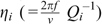 and scattering
 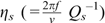 attenuation coefficients were obtained by following a grid search with an interval of 0.001 km−1 to obtain the minimum values of the misfit function Mf for each frequency f (Hoshiba et al., 1991):

where k is the energy value of each distance and j is the number of curves. EOj (rk) and EMj (rk) denote the observed and the theoretical energies, respectively. The error intervals of the two obtained coefficients were obtained using the F distribution test (Draper and Smith, 1998):

where  is the minimum value of Mf (ηs, ηi), p is 2, the number of model parameters (ηs and ηi), and n is the number of energy values. F90 denotes the Fisher distribution function with a confidence level at 90%; this value is more reliable than the previous value, 60% (Asep et al., 2015). The ratios of
 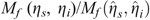 were plotted as the confidence area, as shown by the shaded zones (right panel in Figure 4a). An attenuation value was excluded as unreliable if its error was equal to or greater than the obtained value.
Data and focal depth
This study analysed 12 earthquakes (E1–12 in Table 1) treated not as single events but as combination events in Asep and Chung (2016). In addition, Table 1 also shows four single events from Asep and Chung (2016) (D1–4) because they were used as combination events in Figure 1. Using a crustal model constructed on the basis of refraction profiles (Cho et al., 2006, 2013), Asep and Chung (2016) obtained hypocentral parameters (latitude, longitude, and origin time) by a series of inversions while maintaining a fixed depth. For a suite of focal depths between 0 and 30 km at 0.5-km increments, the root mean square (RMS) residual times were calculated by using HYPO71 (Lee and Lahr, 1975), and the minimum value was chosen. Around the minimum RMS residual time, the depth range was defined as the interval with a difference between the minimum and the residuals of less than 0.05 s (Figure 5). The DM value, the median of the depth range, was used as the event depth in the DSMC method for numerical fitting of MLTWA observations.

|
Results and discussion
The flexible wide-range window enabled us to obtain the values of MLTWA for all single-event data. In addition, more reliable results than with Asep and Chung’s (2016) window were observed for a reduced number of data. As an example, event T1 was attempted for various numbers of observations, 6, 8, and 16, expressed as blue, green, and red symbols, respectively, in Figure 6a. The corresponding confidence zones of the F-test at the 90% level showed improved reliability with increasing number (Figure 6b). In particular, the blue zone was small compared with that of Asep and Chung’s (2016) window (grey colour), although the case of 16 observations showed similar sizes for the red and black colours. The observational lines (dashed lines with three colours in Figure 6a) were fitted by theoretical lines (solid lines with orange colour) using 0.008–0.014 and 0.019–0.025 for our windows of ηs and ηi, respectively, along with lines (black solid lines) of 0.007 and 0.0021 for Asep and Chung’s (2016) window of ηs and ηi, respectively. The ratio, , of the confidence areas for blue, green, red, grey, and black is 3.162, 2.154, 1.389, 3.162, and 1.389, respectively.

|
The results of the MLTWA showed values similar to those of the combined events in Asep and Chung (2016) (Figures 1 and 7). However, the value of E1 showed anomalously lower Qs–1 than those of the combination with D1, which is explained by the small number of data (Table 1). In addition, several values at the frequency of 1.5 Hz were excluded because its error was greater than the value obtained.

|
In Figure 7, the Q–1 values are connected by solid or broken lines for depth ranges (Table 1) smaller or greater than 5 km, respectively. Asep and Chung (2016) showed a depth dependency of Qs–1 with high and low values corresponding to shallow (bluish colours) and deep (reddish colours) levels, respectively (Figure 1a). This depth dependency seems to correlate with our depth range classification, as shown in Figure 7a, in which bluish and reddish solid lines represent shallow (E3) and deep (E10, E11) events and show higher and lower values than those of broken lines (E4 and E12), respectively.
Additionally, as shown by Asep and Chung (2016), the depth dependency was not apparent for Qi–1 and was therefore weakened for Qt–1. The depth dependency of Qs–1 and Qt–1 values can be explained by the closure and healing of fluid-filled cracks in the brittle zone (Mitchell, 1991). This effect for Qi–1 appeared to be compensated for by increasing temperature, due to its heat sensitivity (Asep and Chung, 2016).
Conclusions
The use of single events in MLTWA is a robust tool for the study of crustal Qs–1 and Qi–1. This approach was first attempted by Asep et al. (2015), subsequently improved by Asep and Chung (2016), and finally completed in this study. This study showed a flexible range window to be successfully applied to solely single-event MLTWA. In particular, a more reliable constraint was obtained compared with the previous study, with a reduced number of data. Solely single-event MLTWA may be applicable for investigating seismically stable regions, due to the limitation of available combinations of similar depth events.
Acknowledgements
This research was supported by funds from the Korea Meteorological Industry Promotion Agency under Grant KMIPA2015–7080. Some figures were produced using R (R Development Core Team, 2006) and Generic Mapping Tools (Wessel and Smith, 1998). The authors would like to thank two anonymous reviewers for their suggestions to improve this manuscript.
References
Abdel-Fattah, A. K., Morsy, M., El-Hady, S., Kim, K. Y., and Sami, M., 2008, Intrinsic and scattering attenuation in the crust of the Abu Dabbab area in the eastern desert of Egypt: Physics of the Earth and Planetary Interiors, 168, 103–112| Intrinsic and scattering attenuation in the crust of the Abu Dabbab area in the eastern desert of Egypt:Crossref | GoogleScholarGoogle Scholar |
Aki, K., 1980, Attenuation of shear waves in the lithosphere for frequencies from 0.05 to 25 Hz: Physics of the Earth and Planetary Interiors, 21, 50–60
| Attenuation of shear waves in the lithosphere for frequencies from 0.05 to 25 Hz:Crossref | GoogleScholarGoogle Scholar |
Asep, N. R., and Chung, T. W., 2016, Depth dependent crustal scattering attenuation revealed using single or few events in South Korea: Bulletin of the Seismological Society of America, 106, 1499–1508
Asep, N. R., Chung, T. W., Yoshimoto, K., and Son, B., 2015, Separation of intrinsic and scattering attenuation using single event source in South Korea: Bulletin of the Seismological Society of America, 105, 858–872
| Separation of intrinsic and scattering attenuation using single event source in South Korea:Crossref | GoogleScholarGoogle Scholar |
Badi, G., Del Pezzo, E., Ibanez, J. M., Bianco, F., Sabbione, N., and Araujo, M., 2009, Depth dependent seismic scattering in the Nuevo Cuyo region (southern central Andes): Geophysical Research Letters, 36, L24307
| Depth dependent seismic scattering in the Nuevo Cuyo region (southern central Andes):Crossref | GoogleScholarGoogle Scholar |
Cho, H.-M., Baag, C.-E., Lee, J. M., Moon, W. M., Jung, H., Kim, K. Y., and Asudeh, I., 2006, Crustal velocity structure across the southern Korean Peninsula from seismic refraction survey: Geophysical Research Letters, 33, L06307
| Crustal velocity structure across the southern Korean Peninsula from seismic refraction survey:Crossref | GoogleScholarGoogle Scholar |
Cho, H.-M., Baag, C.-E., Jung, M. L., Moon, W. M., Jung, H., and Kim, K. Y., 2013, P- and S-wave velocity model along crustal scale refraction and wide-angle reflection profile in the southern Korean peninsula: Tectonophysics, 582, 84–100
| P- and S-wave velocity model along crustal scale refraction and wide-angle reflection profile in the southern Korean peninsula:Crossref | GoogleScholarGoogle Scholar |
Chung, T. W., and Asep, N. R., 2013, Multiple lapse time window analysis of the Korean Peninsula considering focal depth: Geophysics and Geophysical Exploration, 16, 293–299
| Multiple lapse time window analysis of the Korean Peninsula considering focal depth:Crossref | GoogleScholarGoogle Scholar |
Chung, T. W., and Sato, H., 2001, Attenuation of high-frequency P and S waves in the crust of southeastern South Korea: Bulletin of the Seismological Society of America, 91, 1867–1874
| Attenuation of high-frequency P and S waves in the crust of southeastern South Korea:Crossref | GoogleScholarGoogle Scholar |
Chung, T. W., Lees, J. M., Yoshimoto, K., Fujita, E., and Ukawa, M., 2009, Intrinsic and scattering attenuation of the Mt Fuji Region, Japan: Geophysical Journal International, 177, 1366–1382
| Intrinsic and scattering attenuation of the Mt Fuji Region, Japan:Crossref | GoogleScholarGoogle Scholar |
Chung, T. W., Yoshimoto, K., and Yun, S., 2010, The separation intrinsic and scattering seismic attenuation in South Korea: Bulletin of the Seismological Society of America, 100, 3183–3193
| The separation intrinsic and scattering seismic attenuation in South Korea:Crossref | GoogleScholarGoogle Scholar |
Del Pezzo, E., Bianco, F., Marzorati, S., Augliera, P., D’Alema, E., and Massa, M., 2011, Depth-dependent intrinsic and scattering seismic attenuation in north central Italy: Geophysical Journal International, 186, 373–381
| Depth-dependent intrinsic and scattering seismic attenuation in north central Italy:Crossref | GoogleScholarGoogle Scholar |
Draper, N. R., and Smith, H., 1998, Applied regression analysis (3rd edition): John Wiley.
Fehler, M. C., Hoshiba, M., and Sato, H., 1992, Separation of scattering and intrinsic attenuation for the Kanto-Tokai region, Japan, using measurements of S-wave energy versus hypocentral district: Geophysical Journal International, 108, 787–800
| Separation of scattering and intrinsic attenuation for the Kanto-Tokai region, Japan, using measurements of S-wave energy versus hypocentral district:Crossref | GoogleScholarGoogle Scholar |
Hoshiba, M., Sato, H., and Fehler, M. C., 1991, Numerical basis of the separation of scattering and intrinsic absorption from full seismogram envelope: a Monte Carlo simulation of multiple isotropic scattering: Papers in Meteorology and Geophysics, 42, 65–91
| Numerical basis of the separation of scattering and intrinsic absorption from full seismogram envelope: a Monte Carlo simulation of multiple isotropic scattering:Crossref | GoogleScholarGoogle Scholar |
Kobayashi, M., Takemura, S., and Yoshimoto, K., 2015, Frequency and distance changes in the apparent P-wave radiation pattern: effects of seismic wave scattering in the crust inferred from dense seismic observations and numerical simulations: Geophysical Journal International, 202, 1895–1907
| Frequency and distance changes in the apparent P-wave radiation pattern: effects of seismic wave scattering in the crust inferred from dense seismic observations and numerical simulations:Crossref | GoogleScholarGoogle Scholar |
Lee, W. H. K., and Lahr, J. C., 1975, HYP071 (revised): a computer program for determining hypocenter, magnitude, and first motion pattern of local earthquakes: US Geological Survey Open File Report 75–311, 113 pp.
Mitchell, B. J., 1991, Frequency dependence of QLg and its relation to crustal anelasticity in the Basin and Range Province: Geophysical Research Letters, 18, 621–624
| Frequency dependence of QLg and its relation to crustal anelasticity in the Basin and Range Province:Crossref | GoogleScholarGoogle Scholar |
R Development Core Team, 2006, R: A language and environment for statistical computing: R Foundation for Statistical Computing, Vienna, Austria. Available at http://www.r-project.org/ (accessed December 2015).
Sato, H., Fehler, M. C., and Maeda, T., 2012, Seismic wave propagation and scattering in the heterogeneous earth (2nd edition): Springer-Verlag, Inc.
Vargas, C. A., Ugalde, A., Pujades, L. G., and Canas, J. A., 2004, Spatial variation of coda wave attenuation in northwestern Colombia: Geophysical Journal International, 158, 609–624
| Spatial variation of coda wave attenuation in northwestern Colombia:Crossref | GoogleScholarGoogle Scholar |
Wessel, P., and Smith, W. H. F., 1998, New, improved version of the generic mapping tools released: Eos, Transactions, American Geophysical Union, 79, 579
| New, improved version of the generic mapping tools released:Crossref | GoogleScholarGoogle Scholar |
Wu, R. S., 1985, Multiple scattering and energy transfer of seismic waves – separation of scattering effect from intrinsic attenuation – I. Theoretical modelling: Geophysical Journal International, 82, 57–80
| Multiple scattering and energy transfer of seismic waves – separation of scattering effect from intrinsic attenuation – I. Theoretical modelling:Crossref | GoogleScholarGoogle Scholar |
Yoshimoto, K., 2000, Monte Carlo simulation of seismogram envelopes in scattering media: Journal of Geophysical Research, 105, 6153–6161
| Monte Carlo simulation of seismogram envelopes in scattering media:Crossref | GoogleScholarGoogle Scholar |