
Application of satellite altimetry for studying the water vapour variability over the tropical Indian Ocean
Fathin Nurzaman A , Dudy D. Wijaya A * , Nabila S. E. Putri B , Noor N. Abdullah A , Brian Bramanto A , Zamzam A. J. Tanuwijaya A , Wedyanto Kuntjoro A , Bambang Setyadji A and Dhota Pradipta A
A
B
Abstract
Satellite altimetry was originally intended for oceanographic and geodetic applications. An uncommon application of satellite altimetry data, demonstrated in this paper, is for atmospheric study by utilising the onboard microwave radiometer. The Wet Tropospheric Correction (WTC) data from the Topex/Jason altimetry mission series (Topex/Poseidon, Jason-1, Jason-2/OSTM and Jason-3) are used, which have spanned nearly 30 years, making them sufficient for climate study. Precipitable Water Vapour (PWV) is derived from the WTC and used to study the atmospheric water vapour variability over the tropical Indian Ocean (TIO). Preliminary analysis is performed by comparing the generated PWV data with the PWV from a dedicated meteorological satellite Aqua, which was found to be comparable with a correlation coefficient of 0.94 for the monthly mean data and 0.74 for the anomaly component. Using standard empirical orthogonal function and composite analysis, the interannual variability of the tropospheric water vapour in TIO is thoroughly analysed. The mechanics and impacts of the two leading modes, the El Niño–Southern Oscillation (ENSO) and Indian Ocean Dipole (IOD) are characterised. Furthermore, the modulation of the atmospheric circulation cell can be monitored. A distinct characteristic is found for the spurious IOD event in 2017 and 2018, which is the forming of a PWV anomaly meridional gradient in the Indian Ocean during June due to the activity of the Southern Indian Ocean Dipole mode. This showcases the potential of using altimetry satellite data for atmospheric study and opens up the possibility of further utilisation.
Keywords: atmospheric circulation cell, atmospheric study, El Niño–Southern Oscillation, Indian Ocean Dipole, microwave radiometer, satellite altimetry, spurious Indian Ocean Dipole, tropical Indian Ocean, tropospheric water vapour.
1.Introduction
The main objective of altimetric satellites is to study ocean circulation through their measurement of sea surface height. Being the only means to observe the sea surface height globally, they have contributed greatly to current understanding of the physical oceanic process, such as the role of large-scale ocean waves (e.g. Cheney et al. 1987; Vinayachandran et al. 2002). Additionally, they have contributed greatly to the field of geodesy in the generation of mean sea surface models and marine geoids for global vertical datum determination (e.g. Sandwell and Smith 2009; Schaeffer et al. 2012). However, the use of the onboard microwave radiometer for atmospheric observation has not been widely explored. This instrument measures the integrated water vapour content along the atmospheric column below the satellite, originally intended to provide the correction for the precise altimetric measurement, hence, this could potentially be utilised to study atmosphere variabilities.
The water vapour in the atmosphere is highly variable in space and time, which makes it complicated to model. Furthermore, the variability produces up to 3–45 cm of bias in the main altimeter measurement (Keihm et al. 1995). This makes meaningful sea level measurement not feasible without eliminating this particular bias beforehand. Therefore, it has been deemed necessary to provide an onboard instrument specifically designated to measure the bias, i.e. the microwave radiometer. To maintain consistent and accurate sea level measurement, the microwave radiometer was designed to maintain a high-precision water vapour measurement. An assessment study by Brown et al. (2004) shows that the uncertainty of wet tropospheric delay derived from measurement of the Jason Microwave Radiometer (JMR) onboard Jason-1 is 0.74 ± 0.15 cm, which surpasses the 1.2-cm requirement (Dumont et al. 2009). A study on the assessment of this instrument in measuring atmospheric variables, such as the integrated water vapour and liquid water content, has been performed and found to be compatible with meteorological satellite observations (Thao et al. 2014). This means that the altimetric satellite’s radiometer is qualified to also be used for accurate atmospheric studies. Furthermore, with the radiometer instrument and validation process continuing to be improved for follow-on satellites, the quality of the retrieved water vapour data in the future is expected to improve, which will further increase the radiometer reliability for atmospheric studies.
Understandably, the onboard radiometer has not been significantly explored for climate study. This is because altimetric satellites are still deficient, particularly in their spatial and temporal resolution, compared to dedicated meteorological satellites. This is specifically caused by the single-point nadir measurement. The onboard radiometer was designed to observe solely the atmospheric column in the nadir direction since its primary function is to measure the wet topographic bias of the nadir-measuring altimeter, thus it does not possess a wide field of view like the imaging radiometer of meteorological satellites. This made the temporal resolution of the altimetry satellite data to be the total repeat cycle, which is the period the satellite takes to go back to the exact same position relative to the earth’s surface, instead of just the subcycle, which is the period it takes for successive passes of the same direction to circle the earth longitudinally. This particular limitation of altimetry satellites is mentioned in Dettmering et al. (2020).
Regardless, it is still of interest to assess the ability of the onboard radiometer for atmospheric observation. The sparse resolution should still be theoretically sufficient to observe a global-scale variability with low frequency, such as the El Niño–Southern Oscillation (ENSO). Since some of the climate variabilities are an ocean–atmosphere coupled process, a synchronous altimeter–radiometer measurement of altimetry satellites, which measure both oceanic and atmospheric variables at the same time might have a great potential in obtaining some valuable information regarding the coupling mechanism. This would lead to improved atmospheric observation from the altimetric satellite by itself, which would improve its atmospheric bias modelling and ultimately lead to improvement in the accuracy of its sea-level measurement. Furthermore, some other variables could be derived from the onboard radar and radiometer instruments. Some satellite altimetry utilises dual-frequency radar, which can be used for various observations, such as estimating rainfall and cloudiness (Bhandari and Varma 1996; Tournadre and Bhandari 2009), air–sea gas fluxes (Goddijn-Murphy et al. 2013) and ionospheric electron content (Ray 2020). The 34-GHz channel of the radiometer can be used to estimate cloud liquid water content (Weng et al. 2011), which increases the potential even more. In this paper specifically, an atmospheric application of satellite altimetry is demonstrated, which is for studying the water vapour variability in the tropical Indian Ocean (TIO) in order to maximally utilise the onboard radiometer.
The Indian Ocean has a significant influence on the equatorial climate as it is associated with the actively oscillating Intertropical Convergence Zone (Philander et al. 1996) and drastic changes in prevailing winds, which cause the surrounding region to experience rainy and dry seasons within a year, also referred to as the monsoonal system. In the interannual timescale, the variability of the atmosphere is intensified with anomalous climate modes affecting the region, namely the Indian Ocean Dipole (IOD) and ENSO. These anomalous climate modes cause the normally high seasonal variation to behave unpredictably, thus increasing the risk of hydrometeorological disasters, particularly events associated with rainfall, such as floods and droughts. Additionally, this unpredictable weather system can also lead to socioeconomic losses through crop failures or infectious diseases. Thus, to be able to mitigate these risks, some understanding of the climate variabilities, such as their mechanism or the spatio-temporal characteristics is necessary.
The IOD is one of the climate variabilities in the Indian Ocean, which is characterised by a dipole structure of sea surface temperature (SST) anomaly (SSTA). This was found to be an inherent variability in the Indian Ocean by Saji et al. (1999) as they analysed the second leading mode that explains 12% of the total variance with a dipole structure from standard EOF analysis on the SST in the region. This anomalous change in SST has various impacts, one of which is the modification of the seasonal upwelling, which affects biological productivity (Lan et al. 2013; Lumban-Gaol et al. 2015). Owing to the ocean–atmosphere feedback mechanism, this would also modify the climate system around the region (Bjerknes 1969; Gill 1980). During the positive phase of the IOD, the zonal gradient of the SST is reversed: the normally wet bordering eastern region becomes drier, which leads to a prolonged summer, increasing the risk of droughts and wildfires (Abram et al. 2021). Concurrently, the normally dry bordering western region experiences more rain than usual, which increases the risk of floods and aids the spread of infectious diseases (Hashizume et al. 2012). In contrast, during the negative phase, the normal zonal gradient is intensified, causing the opposite impact from the positive phase, as the dry western regions get even drier and the rainy eastern regions get wetter (Gebrechorkos et al. 2020; Kurnianingsih et al. 2020).
The ENSO is believed to have remote effects in the Indian Ocean, even though it is a climate mode located in the Pacific Ocean. The IOD was originally assumed to be part of ENSO variability because their phases were frequently synchronised, i.e. extreme IOD often coincides with extreme ENSO (Wallace et al. 1998). On the contrary, it was found to be independent of ENSO by Saji et al. (1999). It was revealed that some instances of extreme dipole mode events did not coincide with ENSO, e.g. the 1994 event. However, it is still of interest to study the possible correlation between them, as the physical proximity between the two oceans allows atmospheric teleconnection through the modulation of the Walker circulation cell (Hameed et al. 2018). Furthermore, they are separated by the Maritime Continent, which allows oceanic pathways between the two through the Indonesian Throughflow (Wijffels and Meyers 2004). Given these circumstances, both events have similar impacts whether in the modulation of the atmospheric circulation cell or the ocean upwelling and downwelling. The coinciding phase would likely reinforce the impact in some regions, which makes the study of both mechanisms significant.
This paper aims to study the water vapour variability of the TIO and further our understanding of the two global modes residing in the region, IOD and ENSO. This will demonstrate the feasibility of using altimetric satellites for atmospheric study. The altimetric missions analysed here are the Topex/Jason altimetry mission series, which includes Topex/Poseidon, Jason-1, Jason-2/OSTM and Jason-3. Nearly 30 years of observation data have been collected, which makes it possible to derive a reliable climatological model needed for the monthly anomaly data computation. Even though some papers have assessed the performance of the onboard radiometer, no study has specifically applied this to atmospheric study. This paper specifically focuses on using the data to analyse the two main climate modes residing in the Indian Ocean, IOD and ENSO. An effort to distinguish the impact of both variabilities is carried out. The methodologies, such as the precipitable water vapour (PWV) derivation and monthly anomaly computation are explained in Section 2. Some data analysis techniques are implemented and the results are described in Section 3, along with the discussion. Section 4 provides a summary.
2.Methods
2.1. Altimetry-derived PWV
This paper used the WTC data of the Topex/Jason mission series, which is the reference altimetric satellite mission. This started with Topex in 1992, followed by the Jason mission series (Jason-1, -2 and -3). They have maintained 30 years of continuous observation in a consistent groundtrack. As the reference altimetric mission, they are used to correct the other non-reference altimetric satellite mission that does not have a long observation period (e.g. Le Traon et al. 1995; Le Traon and Ogor 1998). The reference mission’s satellites are also equipped with a more advanced tracking system to minimise the positional uncertainty as it directly influences the sea surface height measurement.
The along-track sampling spatial separation is ~6 km, whereas the cross-track separation is ~313 km. This is sparse compared to the other satellite altimetry mission’s ground-track, though the sparse groundtrack is a tradeoff for a faster repeat time. The faster repeat time is necessary for the reference altimetric missions in order to accurately estimate some ocean temporal variation (Parke et al. 1987). Note that even with the dense along-track spatial sampling of ~6 km, the actual spatial resolution is strictly determined by the radiometer footprint size, which is conditioned by the antenna size and satellite altitude. The footprint diameter of the lowest frequency band of the Topex Microwave Radiometer (TMR) onboard the Topex satellite is ~42 km (Stewart et al. 1986) and so is that of the JMR onboard the Jason-1 because it has the same length of antenna diameter. The Jason-2 Advanced Microwave Radiometer (AMR) and Jason-3 Advanced Microwave Radiometer 2 (AMR-2) have larger antenna size with a diameter of 1 m (TMR and JMR antenna have 0.6-m diameter) and thus have a finer spatial resolution of ~25 km (Brown 2010; Maiwald et al. 2016). Theoretically, this resolution should be sufficient for capturing large-scale variabilities such as ENSO and IOD. This paper thus assesses the performance of using only the reference missions. This emphasises that higher resolution can still be achieved by using multi-mission satellite altimetry data.
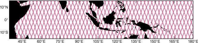
The region of the data being used in this study is the TIO extended eastward to the West Pacific. The distribution of the data can be seen in Fig. 1. This extent is chosen to cover the TIO along with the whole Maritime Continent and a part of the Pacific Ocean where the ENSO variation is very active.
The WTC data were derived from the brightness temperature measured by the onboard microwave radiometer. The microwave radiometer incorporates three channels of measurement: the main channel detects at 23.8 GHz (21 GHz in Topex/Poseidon) for water vapour content measurement, and the other two channels detect at 34 and 18.7 GHz (37 and 18 GHz in Topex/Poseidon), which is meant to provide correction on the main water vapour measurement due to non-rainbearing clouds and wind-driven variations respectively.
The WTC data were acquired from Radar Altimeter Database System (RADS) version 4 developed by Scharroo et al. (2016). RADS is a multi-mission altimetry database that offers an efficient way to query data with various criteria specified by the user, such as period, missions and area of interest in a consistent format. Then, the PWV is calculated from the acquired PWV after applying along-track smoothing to filter out the high-frequency noise by ~16-km averaging (equivalent to three adjacent footprints).
The PWV is one way to measure the atmospheric water vapour content. The definition of PWV used here is the height of total atmospheric water vapour if it is totally condensed in its vertical column. In this study, the PWV is calculated from the WTC using the following equations, which were derived by Askne and Nordius (1987). Tropospheric wet delay (TWD), or the negative of WTC, can be converted to PWV by multiplying it with a coefficient Π, which can be expressed as follows:
with Π defined as:
where Rv is the specific gas constant for the water vapour (461.5254 J kg−1 K−1); ρ is the density of water (997 kg m−3); k′2 = 0.221 K Pa−1 and k3 = 3.739 × 10³ K2 Pa−1 are both atmospheric refractivity constants, values for which can be acquired from the study by Bevis et al. (1994); and Tm is the weighted mean temperature of the atmosphere column (K). Tm is not measured by the altimetry satellites, but was acquired from the model GPT2w (Global Pressure and Temperature 2 wet) by Böhm et al. (2015). However, in this study, a constant Tm value is used for the whole spatial and temporal extent. This is because the calculation of Tm for every single footprint of the altimetry data requires too much computational time using the available resources during the time of this study.
A test was conducted beforehand to determine whether using a constant value of Tm over the TIO would give a significant error to the PWV computation. The detail regarding this test is explained in Appendix A1.
2.2. Altimetry-derived PWV time series generation
The time series of the altimetry-derived PWV was generated by collecting available data within a spatial bin with 3-km radius centred at the crossover or the intersection point of ascending and descending passes. We chose to only study the data in the crossover because they have twice the amount of data as they passed by both ascending and descending passes for each repeat cycle. For the Topex/Jason mission series, the repeat period is ~10 days. Thus, at a crossover point, two data are measured every 10 days or approximately six data for each month. This generates better monthly mean approximation than the non-crossover points, which only have three data per month. Note that the interval between an ascending pass and the next descending pass in a crossover point is not exactly the repeat period divided by two, it varies depending on the latitude of the crossover point. As an ascending or descending pass by itself has an exact repeat period, the merging of the two will result in a pairwise evenly spaced temporal sampling; it is evenly spaced if we look pair by pair. These peculiar sampling characteristics are worth mentioning when performing a thorough analysis because this could affect how a certain signal is captured. Nevertheless, the temporal resolution is still considerably better. However, using only data at the crossover results in degrading the spatial resolution as the other observed footprints (not in the crossover) are disregarded. For the tropical region (15°S to 15°N), the zonal and latitudinal separation of the crossover points are ~313 and ~415 km respectively. This is considered sparse but should still be able to sufficiently capture the global-scale variability, such as ENSO and IOD. For illustration, the distribution of the crossover points over the TIO can be seen in Fig. 5b or 5c.
2.3. Monthly mean anomaly computation method
To extract the ENSO and IOD signal from the data, normal components must be eliminated, leaving only the anomaly. These components depict the normal state, or the state without any anomalous variation, based on the averaging of a long period of data, preferably decades, to eliminate inter-seasonal variabilities. As such, this component is also generally referred to as the climatology. The normal components defined in this study are the long-term mean and trend, as well as the regularly occurring seasonal oscillation. Therefore, for this study, the anomaly is computed by eliminating the long-term mean, trend and seasonal components from the PWV time series. Hence, the following mathematical equation is used to compute precipitable water vapour anomaly (PWVA):
where t is time, M is the PWV long-term mean, and L and S are the linear trend and seasonal components of the PWV time series respectively. The M is acquired simply by averaging the data. The parameters for the trend and the seasonal component are estimated using simple least squares adjustment. The simple linear model is used for the trend component. For the seasonal component, the first three harmonics of the annual cycle are used, therefore L (Eqn 4a) and S (Eqn 4b) are defined as follows:
and
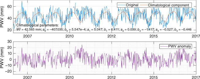
where atr and btr are the constant and the gradient term of the linear trend component respectively. T is 365.25 days or a 1-year period, thus ak and bk for k = 1, 2 and 3 are the sine and cosine terms for the first three harmonics of the annual cycle. The period chosen to estimate the average (M) and the other parameters using least squares adjustment is exactly 28 years, which spans from September 1993 to August 2021. Exactly a round number of years for the base period is necessary to minimise bias from a non-complete annual cycle and its harmonics. The PWVA time series is then computed using Eqn 3 and 4a for the whole period and each point independently. One example of the time-series PWV data along with the estimated climatological component and the extracted anomaly component is shown in Fig. 2. For the monthly values, a simple averaging is performed for each month using all the available data that exist within the month.
3.Results
3.1. Comparison with data of a dedicated meteorological satellite
Before analysing the variability of water vapour in TIO, the accuracy of the generated monthly mean values is assessed first by comparing them with a verified dataset collected from a dedicated meteorological satellite. The AIRS3STM v.7 total precipitable water dataset (AIRS Project 2019) is used here. The data are collected from the sun-synchronous Aqua satellite that observes the same area twice a day at consistent local time, thus receiving consistent lighting from the sun, which is ideal for weather observation. The twice-daily observation also ensures reliable monthly mean data as the diurnal variation can be resolved and then removed accurately. The water vapour is observed using the Atmospheric Infrared Sounder (AIRS), an infrared and visible–near-infrared spectrometer with high spectral resolution. The dataset has a spatial resolution of 1° and covers the whole of the earth’s surface. The PWV monthly mean value of the AIRS3STM v.7 is computed and spatially interpolated to acquire the PWV values that collocate with the altimetry-derived PWV data in the crossover points all over the TIO (30–90°E, 15°S–15°N). The comparison between the two data is shown in Fig. 3. High similarity between the two data is apparent with a Pearson correlation coefficient value of 0.94. The long-term mean value, the M as defined in Eqn 3, is also compared, denoted with the green plus symbol in the scatterplot. A difference in the mean value would indicate a systematic difference such as an offset between the two data, which indicates a possible processing error. In Fig. 3, the mean values scatterplot coincides with the x = y line, which validates that there is no processing error.
Scatterplot of the monthly mean PWV (a) and monthly anomaly PWV (b) derived from satellite altimetry data and AIRS3STM v.7.
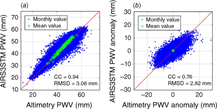
This shows that the altimetry-derived monthly mean PWV data are in good agreement with the reference verified AIRS3STM v.7 data. However, it is well known that seasonal variation in the Indian Ocean is responsible for a high percentage of the total variance because of the monsoon regime that occurs in the region. In analysing the inter-annual variation like IOD and ENSO, the anomaly values would be used, which is the monthly mean subtracted by the climatological components that contain the seasonal variation (Eqn 3). The PWVA comparison is shown in Fig. 3b. In this analysis, the linear trend and seasonal variation are calculated using the same base period for the two data to ensure that they actually represent the same anomaly variation. The base period is 2002–2021, which is the longest period available for both datasets.
The correlation coefficient of the anomalies declined to 0.76 for the anomaly component values. The RMSD is 2.82 mm whereas the PWVA standard deviation is 4.34 mm. This gives a RMSD to standard deviation ratio of 0.65 which is considered high and might significantly affect the analysis result. The unsolved diurnal variation possibly contributed to the high RMSD.
The diurnal variation in the tropics contributes ∼15–20% of the total variance of the precipitation (Yang and Slingo 2001). This diurnal variation is not completely eliminated from the computed monthly mean PWV because of the sampling characteristic of the Topex/Jason satellite; there are too few samples within a month and their sampling repeat period is almost an exact round number of days, thus the diurnal variation cannot be easily removed. For the AIRS3STM dataset, which is observed twice daily by the Aqua satellite, the diurnal variation can be safely removed.
In the tidal modelling application of satellite altimetry, a sub-diurnal variation is generally resolved by utilising their aliased frequency. This is possible since the orbit of the altimetric satellites, such as Topex/Jason, was designed to have a repeat period that would alias the diurnal or semi-diurnal variation to a desirable frequency (Parke et al. 1987). However, unlike tidal constituents, we cannot expect the diurnal variation of the atmospheric water vapour to be an ideal sinusoid-like sea level, which is strongly driven by the gravitational force of regularly revolving celestial bodies. Theoretically, the diurnal cycle of the atmospheric water vapour is far more complex as it is also heavily influenced by other factors such as the highly transient weather systems. In other words, the variation is not an ideal sinusoid with a constant amplitude that would simply be aliased like the diurnal sea level variation. Using the crossover point that merges ascending and descending passes as explained in Section 2.2 would help in reducing this bias, as the interval between an ascending and the next descending pass in the crossover is not generally a round number of days. To be sure, the significance of the bias can be inferred through comparison with a reliable dataset as is done here.
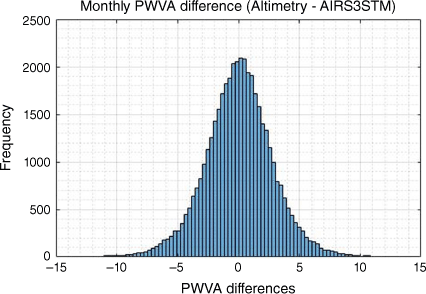
The comparison shows that the difference becomes quite significant when comparing the monthly anomaly values. This could be a problem when we try to study ENSO and IOD variation from the data. Therefore, further analysis of the differences is needed. Fig. 4 shows the histogram of the differences between the monthly PWVA derived from satellite altimetry and the AIRS3STM dataset. The difference appears to be normally distributed with a symmetrical bell shape. The peak value is also close to zero. This distribution signifies that the differences are mostly caused by random error. The standard deviation is 2.82 mm whereas the original uncertainty of the altimetry-derived PWV is 1.20 ± 0.24 mm as discussed in Section 2.1. There are random errors from other sources, which could contribute to the increasing standard deviation from the original uncertainty, such as the uncertainty in the reference dataset AIRS3STM and the Tm value that was used for the PWV computation. So, it was concluded that the RMSD is mostly caused by the normally distributed random errors and the unresolved diurnal variation would not significantly affect the analysis results. Nevertheless, for further analysis, the RMSD value is considered to be the standard error of the altimetry-derived monthly PWVA data and would be used when performing the significance tests for the analysis results.
3.2. Interannual modes identification
We performed standard empirical orthogonal function (EOF) analysis on the altimetry-derived PWVA values to find and separate the underlying dominant variations from the data. The results can be seen in Fig. 5. The first leading principal component (PC1) explains 18.3% of the total variance and has a dipole structure (Fig. 5b), whereas the second one (PC2) accounts for the basin-wide homogeneous variability (Fig. 5c) and explains 12.3% of the total variance. The variance percentage of the remaining principal components significantly dropped after the second one (6.7%), which presumably indicates that just the local variations are not significantly related to ENSO or IOD. Slightly different characteristics are seen compared to the generated SSTA modes in Saji et al. (1999), in which the first principal component accounts for the basin-wide variability with uniform polarity, described as part of the ENSO variation (Wallace et al. 1998), with 30% of the total variance. By contrast, the second principal component with 12% accounts for the dipole structure, which is then described as the IOD.
Time series of the first two principal components, PC1 and PC2 (a), and their corresponding principal loading maps (b and c) from a standard EOF analysis on the altimetry-derived PWV around TIO and the Maritime Continent.
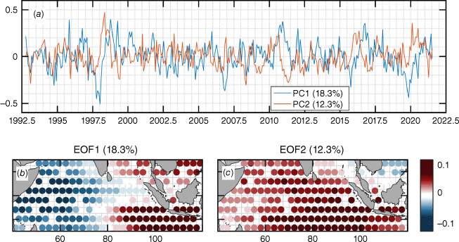
The Pearson correlation coefficients of PC1 and PC2 with the indices that represent ENSO and IOD are computed to see how they correlate. The indices used here are the Oceanic Niño Index (ONI) for ENSO and Dipole Mode Index (DMI) for IOD. These indices are computed from the SSTA values over a specific region: the central Pacific for ONI and the difference between west and south-east TIO for DMI. Therefore, this analysis is intended to determine how the SSTA modes affect the PWVA ones.
The results can be seen in Fig. 6. The correlation values with various lags are also computed to identify any sort of delayed reaction. The results show that PC1 correlates similarly highly with both ONI and DMI with zero lag. However, PC2 only significantly correlates with ONI, with the highest correlation value at 5-months lag. This means that the ENSO has a remote delayed reaction to the PWV in the TIO.
Correlation analyses of the first two PCs of altimetry-derived PWVA to ONI and DMI. The graph shows the Pearson correlation coefficients of PC1 (a) and PC2 (b) to the two climate indices over varying lags.
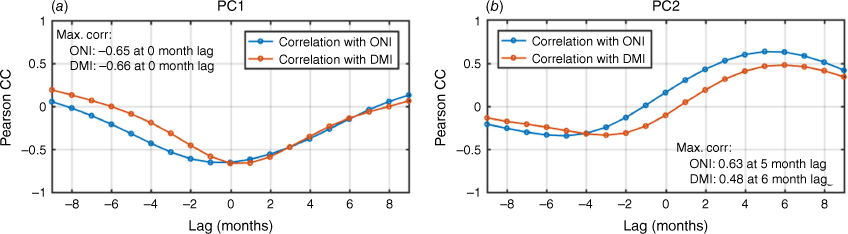
The El Niño composite maps in Saji and Yamagata (2003, fig. 14g–h) show the anomalous easterly in the eastern basin, which signifies the weakening of the convergence zone over the Maritime Continent. This weakening of the convergence zone should emerge in the PWVA field since PWVA is a proxy variable for convergence zones. The weakening convergence zone would cause a decrease of PWV over the Maritime Continent and an increase in the west to the central Indian Ocean, hence creating the zonal gradient structure of PWVA. This explains why PC1 correlates significantly with ONI. The SSTA is not affected much by the anomalous zonal wind, so it maintains the basin-wide property and thus is captured in the first EOF with a basin-wide homogeneous structure. Furthermore, the basin-wide SSTA changes in the Indian Ocean are delayed compared to the changes in the Pacific Ocean, which explains the high lag correlation of PC2.
The ONI being captured by two different modes, in this case, the PC1 and PC2, could mean that the effect of ENSO on PWV has a propagation feature. Studying the exact spatiotemporal characteristics is indeed challenging with standard EOF analysis. Therefore, to see the spatiotemporal structure more clearly, a composite analysis is performed.
A composite analysis is performed by averaging all the data that fall within certain periods, which are typically the periods where a particular event of interest is occurring. This way, all components unique to the event are captured, whereas the other components not correlated with the event get diminished or even eliminated if the number of samples is large enough. Hence, the selection of the samples for the composite analysis to derive the composite map is important. From the whole studied period, there are actually very few samples to be taken for the generation of IOD composite maps. There are 10 events of extreme IOD, with seven of them being positive IOD and only three being negative IOD. This only has a simple classification using the DMI values, so it still includes the 2017 spurious positive IOD event (Zhang et al. 2018), which means only six reliable positive IOD samples are available.
Furthermore, some of the years coincide with extreme ENSO events (four out of six), and picking only pure IOD events leaves too few samples for an effective composite analysis. To mitigate this, we implement a more robust composite analysis method that uses the median instead of the mean. Using the median instead of the mean makes the composite results more robust against noise and allows for fewer samples to be used (Brown and Hall 1999). For the ENSO composite maps, sample selection can be done without any trouble since there are enough ENSO events that do not coincide with IOD within the studied period. In the end, the composite maps of positive IOD, El Niño and La Niña are generated. For the negative IOD, because of the lack of samples that can be selected, 1996 pure negative IOD events are used instead to represent the composite map of negative IOD. Each composite map includes the 2-month average from May–June to November–December following the positive IOD composite map in Saji et al. (1999) so we can compare them. The generated composite maps are shown in Fig. 7. The statistical significance test of the composite maps is performed using Monte Carlo simulations with the previously computed RMSD of 2.82 mm as the standard error. More detail regarding the significance test is explained in Appendix A2.
Composite maps of the altimetry-derived PWVA corresponding to the interannual climatic events; Positive IOD (a–d), Negative IOD (e–h), El Niño (i–l), and La Niña (m–p). The PWVA value is shown in shades with 1-mm intervals and contours of 2-mm intervals. The contours for negative values are hashed and for zero values are omitted. Regions with insignificant PWVA values in 90% confidence interval are darkened.
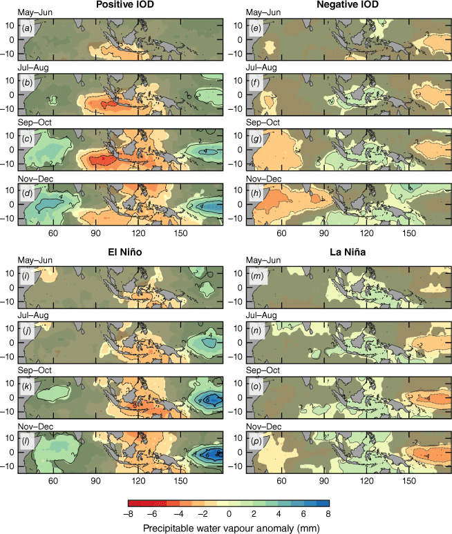
The positive IOD composite maps consisting of the years 1994, 1997, 2006, 2018 and 2019 are shown in Fig. 7a–d. Note that years of positive IOD that coincide with El Niño are still included here, which are 1997, 2006 and 2018. The composite computation method hopefully minimises the El Niño contamination. Because it was also the year of extreme El Niño, 2015 is not included as it could significantly contaminate the composite map despite the robust computation method.
The beginning of IOD events is characterised by the lowering of PWV values around the south-eastern basin, which include the south coast of Java and the south-west coast of Sumatra (Fig. 7a). This is caused by the cooling of SST in the regions as can be seen by the composite map in Saji et al. (1999). The increasing of PWV in the western basin appears later in July–August (Fig. 7b). This is also in good agreement with the wind anomaly field of the composite map of Saji et al. (1999), in which during that month an anomalous easterly appears that signifies the weakening of the circulation cell that caused the increase of evaporation in the western basin. Then the anomaly peaked in September–October forming a clear dipole structure (Fig. 7c), similar to the SSTA field. This similarity with the SSTA field indicates that the SST–PWV feedback (Gill 1980) has a significant role in the mechanism of IOD. The negative PWVA region expands covering almost the whole Indonesia region with the southern part being more affected, especially in the regions close to the south-eastern pole, i.e. Java and South Sumatra. The positive PWVA seems to cover the entirety of East Africa that borders the Indian Ocean. During the dissipation phase in November–December (Fig. 7d), the east pole dissipates quicker than the west, reflecting the seasonal phase-locking mechanism: the warming of the eastern basin caused by the reduced cloudiness and the increasing solar flux in the equator when entering autumn (Saji et al. 1999). This, in turn, deepens the thermocline and reduces the surface wind–SST feedback that maintains the anomalous pattern (Xie and Philander 1994). The area of the significant PWVA is larger than the SSTA in this phase, which indicates that the impact on PWV persists longer than on SST. This is accompanied by the persisting anomalous easterly as seen in the composite map of Saji et al. (1999).
For the negative IOD, the composite analysis cannot be done effectively as there are only three occurrences of negative IOD events within the observational period. Out of the three events, one coincides with La Niña (in 1998) and one with a weak La Niña event (in 2016). However, for the sake of studying the PWVA structure during negative IOD, the 1996 IOD is used, which is the one event not accompanied by La Niña. This has been confirmed by Meyers et al. (2007) as they classified ENSO and IOD events using a multivariate index, so the variability from ENSO can be considered filtered out for this particular year. Additionally, the DMI is exceptionally high (negative) for this year and, thus, could serve as a good representative of a negative IOD event.
The PWVA maps during negative IOD in 1996 are shown in Fig. 7e–h. The spatial structure is similar to the positive IOD but with an opposing sign; we can see here that northern Australia is not affected in autumn, which is supposed to be the peak months (Fig. 7g). This indicates that the affected north of Australia in the positive IOD composite map is most likely due to El Niño contamination. The negative PWVA in the western basin actually has higher amplitude during November–December (Fig. 7h) and the positive ones expand, meaning that the strengthening of the atmospheric circulation cell persists longer than the reversal during positive IOD. However, more samples are needed to infer if this is the general characteristic of negative IOD or just unique to the 1996 event.
The El Niño composite map is shown in Fig. 7i–l. The chosen years to generate this composite map are 2004, 2006, 2009, 2015 and 2020. These are all the pure El Niño events, with the exception of 2006. The IOD effect of that year is assumed be eliminated by the robust composite map generation method.
In the El Niño composite map, we can finally see the actual structure during an El Niño event. The signature ENSO characteristic, which is the high PWVA in the western Pacific, is more apparent here compared to that in the positive IOD map (Fig. 7a–d). The zonal gradient that caused the ONI is highly correlated with PC1, which has a dipole structure. The spatial structure clearly differs from that of IOD. The high negative PWVA region is more shifted to the east and clearly does not form a peak in the centre of the south-eastern basin like the IOD. The peak PWVA value is actually located in the centre of Indonesia. So, it can be described as just a zonal gradient across the Indian Ocean because it does not form a dipole structure as the IOD does. During the initiation phase (Fig. 7i), the lowering of PWVA starts in the centre of Indonesia and the northern tip of Australia, which signifies that the cooling of SST starts in this region as opposed to the IOD that starts around the south coast of Java, see fig. 2a in Saji et al. (1999). This is because the IOD is associated with the reflected coastal Kelvin wave on the Indonesian coastline whereas the ENSO is associated with the Kelvin wave on the Australian coastline (Saji and Yamagata 2003).
The affected regions during El Niño clearly differ from the IOD: in Indonesia, the central part is more affected, which includes the centre to the east of Java and southern Sulawesi whereas Sumatra is not affected. The impact extends to the north, which covers the Philippines along with a part of the South China Sea and the Philippine Sea. By contrast, in the western boundary, East Africa does not get a significant increase in PWV values such as during an IOD event. However, the progression period within a year is similar to that of IOD, i.e. the initiation that begins in boreal spring peaks in autumn and dissipates in winter. This indicates that a similar phase-locking mechanism to the IOD also operates to maintain El Niño events.
The La Niña composite map shown in Fig. 7m–p uses 1999, 2007, 2010, 2017 and 2020 La Niña as the samples. These are all pure La Niña years, so the actual characteristics of La Niña should be captured accurately here. Similar characteristics to El Niño are apparent but with opposing signs to the PWVA values. This increases the certainty of the difference in spatial structure between ENSO and IOD as shown from the composite maps of El Niño compared to positive IOD: a greater impact on the centre of Indonesia and north of Australia and low to no impact over the east of Africa.
The composite maps show the general characteristics of extreme ENSO or IOD, although for each occurrence there could be a significant difference because of some other factors. The reversal of the circulation cell over the TIO might not happen even if the SSTA dipole structure is formed, which is the case in 2017. To analyse this further, a new monitoring index is generated using the altimetry-derived PWVA. Adopting the method for DMI computation, this new index uses the PWVA difference between the western region (45–65°E, 2.5°S–2.5°N) and the south-eastern region (90–105°E, 5–11°S) of TIO. These regions are chosen because these are the dipole peaks of PC1 as the PWVA dipole mode (Fig. 5b). Since PWV is a proxy variable for the convergence zone, this index, hereafter referred to as the PWV Dipole Gradient (PWVDG), is thus meant to specifically depict the circulation cell above the TIO. Positive PWVDG means the reversal of the circulation cell and negative means the strengthening of the normal circulation cell.
Since PWVDG can monitor the state of the convection cell, specifically the Walker circulation cell over the Indian Ocean, which is modulated by IOD and ENSO, this index thus serves to monitor the atmospheric coupling of anomalous climate events. Analysing this index together with DMI and ONI shows how the atmospheric circulation, which is associated with the Bjerknes feedback that explains the ocean–atmosphere coupling, progresses along with the events.
The time series of the PWVDG is shown in Fig. 8. Note that 3-month-running mean is performed first to the DMI and PWVDG to equalise the spectral components with ONI. The ONI involves a 3-month running mean in its computation, supposedly to remove any intra-annual variations. The PWVDG correlates highly with DMI with a Pearson correlation coefficient of 0.73. This high correlation is clearly shown in the time-series plot by some extreme DMI values being accompanied by high PWVDG. This means that when the SSTA forms a dipole in the TIO, the circulation cell or the PWVA field is almost always modulated accordingly. This is true for the exceptionally long-lasting high DMI – specifically during which the DMI peak exceeds ±1σ for at least 3 months. In other words, the Bjerknes feedback will only be initiated after these criteria are fulfilled. Interestingly, the role of the ENSO is also seen here. During some instances when the DMI is high but the ONI is low or in an opposing sign, the PWVDG value is suppressed, such as in the years 1996, 2004, 2005 and 2017 with the last being an extreme case.
Time series of PWVDG superimposed with ONI and DMI. All values are normalised with their respective mean and standard deviation.
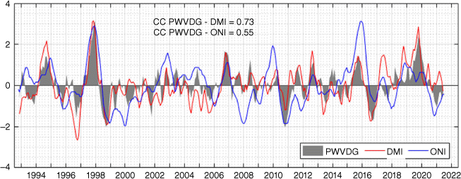
The anomalous year 2017 was studied by Zhang et al. (2018). They show that the high DMI value was driven by the activity of another mode, which is the Sub-tropical Indian Ocean Dipole (SIOD). In early 2017, this mode reaches its peak, and the negative SSTA pole located in the south-eastern Indian Ocean (105°E, 15°S) has a wide spatial structure that reaches the south-east TIO and, thus, creates a gradient structure in TIO, hence the high DMI value. This lasts until the autumn of that year when the subtropical dipole structure finally dissipates. Normally, this would lead to a positive IOD by the shifting of the negative SSTA pole equatorward (Huang et al. 2021). However, this does not happen in that year. Instead, sudden warming in the eastern TIO occurs, which gives a sudden drop to the DMI value later in the year, which might be caused by the ENSO forcing from the Pacific or an intra-annual mode (Zhang et al. 2018). This year is thus dubbed a spurious IOD event.
In 2018, the DMI is high and the ONI reaches 1σ with the same sign, which is supposedly favourable for the initiation of SST–PWV feedback. However, this is not the case as the PWVDG is low. Upon further inspection using surface winds and SST data, positive SIOD occurs in this year, just like 2017. The wide eastern pole reaches the south-eastern pole region of the IOD, thus increasing the DMI value. This is followed by a positive IOD in 2019, as in the following year, just as theorised by Huang et al. (2021). For further insights, the SSTA and surface wind maps along with the altimetry-derived PWVA maps are displayed in Fig. 9. Two specific months are displayed: June, supposedly the month for the IOD initiation phase, and October, supposedly the peak phase as described by Saji et al. (1999) and as also shown in the previous composite analyses.
Comparison of SST anomaly, surface wind and altimetry-derived PWV fields between the high DMI events in 2017, 2018 and 2019 during the initiation phase month in June (a–f) and the peak phase month in October (g–l).
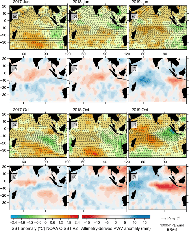
In June of 2017, SIOD activity is clearly seen. The emanating Kelvin wave from the Sumatran west coast that signifies the start of IOD is not apparent here, the high SSTA region is just the extension of the eastern dipole of the SIOD whose peak is located in the south, closer to Australia (Fig. 9a). In 2018, however, the coastal Kelvin wave has no significant SIOD activity (Fig. 9b), similar to that of a normal IOD initiation phase as shown in the composite map by Saji et al. (1999; fig. 2a), although without the zonal SSTA gradient – unlike what happened in 2019 (Fig. 9c), which clearly follows the composite maps. The PWVA maps (Fig. 9d, e) show a more distinct characteristic that differentiates these 2 years as compared to the normal IOD in 2019 (Fig. 9d–f). Both 2017 and 2018 show a region with high negative PWVA values in the centre of TIO and positive values in the southern side. This meridional gradient can be interpreted as the modulation of the meridional circulation cell due to the activity of the SIOD. This could be a hint for identifying another spurious IOD event from as early as its initiation phase.
During the peak phase in October, in 2017 and 2018, the normal equatorial westerly is still maintained despite the SST zonal difference that causes the high DMI value (Fig. 9g, h). We can also see more clearly here the SIOD activity in 2018 from the SST structure, which is not visible for June, though visible in the PWVA map as the meridional gradient. As such, the low SST in the south-eastern basin is just an extension of the eastern pole of the SIOD just like in 2017. The maintained equatorial westerly means that the reversal of the circulation cell identical with a positive IOD event does not occur, which is seen more clearly in the PWVA maps as the dipole anomaly does not develop (Fig. 9j, k). In comparison, the equatorial surface winds blow westward in 2019 (Fig. 9i), causing the reversal of the circulation cell that is represented by the forming of a dipole mode in PWVA field (Fig. 9l). Perhaps a change in the dipole region of the SST for the DMI computation could be made in order to more accurately identify the occurrence of IOD events.
4.Discussion
A thorough analysis of the water vapour variabilities in the TIO is performed using the PWV derived from the altimetry satellite’s microwave radiometer. A preliminary analysis is conducted to see whether the arbitrary sampling of altimetry in the crossover gives a significant bias to the monthly mean calculation. Comparison with water vapour data, specifically AIRS3STM from a dedicated meteorological satellite Aqua shows strong similarity, signified by the high Pearson correlation coefficient value (>0.9) and low RMSD. Comparing the data again but for the anomaly component, gives significantly lower similarity with a 0.76 Pearson correlation coefficient. However, the differences are normally distributed, which signifies that they are mostly caused by random rather than systematic errors from the sampling method. The computed RMSD of 2.82 mm is then considered to be the standard error of the measurement in further analyses for the statistical significance test.
A standard EOF analysis is performed to determine any PWV variability modes that exist in the TIO. Two dominant modes are found, with the first mode having a dipole spatial structure that explains 18.3%, and the second one having a basin-wide homogeneous characteristic with 12.3%. Correlation analysis suggests that PC1 correlates with both IOD and ENSO whereas PC2 is a lagged impact from ENSO. The composite analysis is performed to see the spatiotemporal characteristics more clearly. The ENSO composite maps display the zonal gradient structure that aids the strong correlation of ONI with PC1, which has a dipole structure. The spatial structure clearly differs from the IOD – it does not actually form the dipole shape, with the most noticeable being the absence of the south-eastern pole located close to the south-west coast of Sumatra.
Overall, good agreement is found between the generated composite maps and those from previous studies, specifically the SSTA and surface wind maps in Saji and Yamagata (2003). The PWVA field correlates highly with the wind anomaly field, as both describe the structure of the zonal circulation cell. Additionally, ONI correlates highly with PC1 because of the modulated circulation cell during the mature phase of ENSO. The modulated circulation cell over the TIO is characterised by the anomalous equatorial surface wind (Saji and Yamagata 2003, fig. 14g–h) as well as the zonal gradient structure of PWVA, hence the high correlation between them. However, the high lag correlation of ONI with PC2 is caused by the lagged basin-wide uniform polarity SSTA, see fig. 14gh in Saji and Yamagata (2003), which in turn causes a basin-wide homogeneous modulation of PWVA because of the increased evaporation.
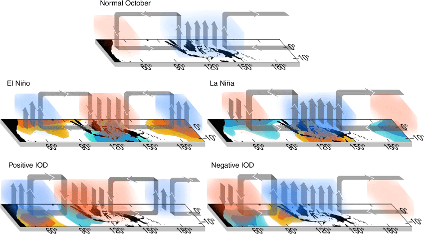
Based on the gathered results, a simple schematic diagram that explains the overall variations of atmospheric water vapour over the TIO is given in Fig. 10. The impact similarity of the two modes is the modulation of the Walker circulation. As such, the co-occurrence of the two modes, such as positive IOD with El Niño or negative IOD with La Niña can further amplify the modulation of the Walker circulation, which would increase the hydrometeorological disaster risk in the nearby regions. In fact, this co-occurrence is more likely to occur based on the time-series graph in Fig. 8.
The schematic diagram for the interannual variability of the Walker circulation cell. The colour shading on the basemap symbolises SSTA with blue for negative SSTA and orange for positive. The opaque shade symbolises the atmospheric water vapour content, red means dry or low water vapour content and blue means the opposite.
From the composite maps, the impact on PWVA during IOD and ENSO can be summarised as follows: the IOD affects the south-western part of Indonesia since the peak anomaly is centralised in the south-eastern basin of the Indian Ocean, clearly affecting south Sumatra and Java more than other regions, whereas the ENSO impact is more in the centre of Indonesia with a greater effect on South Sulawesi and East Java. The milder impact of ENSO can also be seen in the Philippines and the surrounding ocean. This impact is also shown in the positive IOD composite maps and is highly likely the cause of the coinciding El Niño–positive IOD event still included in the composite samples, because the 1996 pure negative IOD event clearly does not show this impact. East Africa appear to be only affected by IOD, whereas the impact of ENSO can be seen only around the Somalian coast.
Using the new PWVDG index shows that the Bjerknes feedback is initiated only when the DMI is high and long-lasting. A simple statistical analysis of the time series suggests that the coupling would initiate if the DMI value exceeds ±σ for at least 3 months. The ENSO also has a role in modulating the strength of the atmospheric impact in which a high DMI event with low ONI would suppress the PWVDG value. It is also found that the DMI value can be amplified by another mode, which is the SIOD located in the southern Indian Ocean. The extreme instance of positive SIOD could increase the SST in the IOD south-eastern pole region, which then increases the DMI value; however, the circulation cell is not affected as shown by the low PWVDG value, and such cases occur for years 2017 and 2018. Further analyses of the SSTA and surface wind maps (Fig. 9) show that the supposed zonal surface wind anomaly does not occur, which indicates that the circulation cell is not modulated. Compared with the matured El Niño event in 2019 (Fig. 9i), it is clear that the SSTA spatial structure differs. In 2019, the extremely high SSTA region emanates from the west coast of Sumatra as Kelvin waves, which is the theoretical origin of an IOD event (Saji et al. 1999; Saji and Yamagata 2003). Perhaps in the computation method of the DMI, more emphasis is needed on the coastal region of the TIO eastern boundary for the south-eastern pole SSTA value for the index to be able to truly capture IOD events that reach a mature phase. Moreover, analysing the initiation phase in June shows a clear characteristic of the two spurious IOD events: the PWVA meridional gradient; and the negative PWVA region in the centre of the TIO with positive PWVA to the south (Fig. 9j, k). This characteristic might be useful to predict another spurious IOD year before the supposed peak month around October. This emphasises the usefulness of using the altimetry-derived PWVA data, as the characteristics cannot be seen in the SSTA-surface wind maps, specifically for the year 2018.
5.Conclusion
The feasibility of using radiometer data of altimetry satellites was demonstrated in this paper. The long series of data spanning 30 years is advantageous for generating a reliable climatological model and composite maps, which is needed for analysing anomalous climate events. The sparse data resolution still allows for a thorough analysis of large-scale global variabilities such as IOD and ENSO. Using the altimetry-derived water vapour data, the water vapour variability over TIO was studied, specifically showing how the atmospheric circulation cell was modulated by the climate modes. One notable finding was the characterisation of the spurious IOD years, such as 2017 and 2018. Similar PWVA characteristics were seen in these 2 separate years from as early as June, which is the theoretical IOD initiation phase month. This gives a possibility for early identification of spurious IOD events.
Compared with meteorological satellite imagery, satellite altimetry data are compromised due to limited spatial and temporal resolution. However, this resolution should theoretically be able to capture large-scale variability and the performance was showcased in this paper. The long continuity of data is especially useful as anomalous climatic events can be well analysed. Satellite altimetry has been measured for 30 years and is planned to continue. Note that this is longer than some of the modern meteorological-dedicated satellites. As more time passes, the ability to capture anomalous events of longer time-scales will improve, such as the interdecadal variation that is very significant in climate study. Furthermore, this research only uses the Topex/Jason altimetry mission series, and higher resolution can potentially be achieved by combining different currently available satellite altimetry missions. Therefore, further research on the utilisation of altimetric satellites is recommended for more advanced atmospheric observation. The synchronous altimeter–radiometer measurement that is unique to satellite altimetry is especially interesting as it synchronously measures both sea surface height and water vapour. This synchronous measurement of oceanic and atmospheric parameter should theoretically be useful in studying the ocean–atmospheric coupling mechanism and obtaining new insights, which is not possible when using only meteorological satellite data. Additionally, it is worth mentioning that other variables can be obtained from the two instruments, such as the significant wave height and wind speed from the altimeter and cloud liquid water content from the radiometer, which shows even greater potential of altimetry satellites. As such, altimetric satellites are expected to make more contributions in the future to study of the atmosphere, complementing the already existing dedicated meteorological satellites.
Data availability
The datasets used or analysed during the current study are available from the corresponding author upon reasonable request. A preprint version of this article is available in Nurzaman et al. (2022).
Acknowledgements
The authors express their gratitude to TU Delft, NOAA and Altimetrics LLC for providing the altimetry data through RADS server; NOAA for the ONI and DMI data; NASA GES DISC for the AIRS3STM v.7 dataset; NOAA for the OISST V2 dataset; and Copernicus Climate Change and Atmosphere Monitoring Services for the ERA-5 1000-hPa wind dataset.
References
Abram NJ, Henley BJ, Sen Gupta A, Lippmann TJR, Clarke H, Dowdy AJ, Sharples JJ, Nolan RH, Zhang T, Wooster MJ, Wurtzel JB, Meissner KJ, Pitman AJ, Ukkola AM, Murphy BP, Tapper NJ, Boer MM (2021) Connections of climate change and variability to large and extreme forest fires in southeast Australia. Communications Earth & Environment 2, 8.
| Crossref | Google Scholar |
AIRS Project (2019) Aqua/AIRS L3 monthly standard physical retrieval (AIRS-only) 1 degree x 1 degree V7.0 (AIRS3STM). (Goddard Earth Sciences Data and Information Services Centre : Greenbelt, MD, USA) [Dataset] 10.5067/UBENJB9D3T2H
Askne J, Nordius H (1987) Estimation of tropospheric delay for microwaves from surface weather data. Radio Science 22(3), 379-386.
| Crossref | Google Scholar |
Bevis M, Businger S, Chiswell S, Herring TA, Anthes RA, Rocken C, Ware RH (1994) GPS meteorology: mapping zenith wet delays onto precipitable water. Journal of Applied Meteorology 33(3), 379-386.
| Crossref | Google Scholar |
Bhandari SM, Varma AK (1996) Potential of simultaneous dual-frequency radar altimeter measurements from TOPEX/Poseidon for rainfall estimation over oceans. Remote Sensing of Environment 58(1), 13-20.
| Crossref | Google Scholar |
Bjerknes J (1969) Atmospheric teleconnections from the Equatorial Pacific 1. Monthly Weather Review 97(3), 163-172.
| Crossref | Google Scholar |
Böhm J, Möller G, Schindelegger M, Pain G, Weber R (2015) Development of an improved empirical model for slant delays in the troposphere (GPT2w). GPS Solutions 19(3), 433-441.
| Crossref | Google Scholar |
Brown S (2010) A novel near-land radiometer wet path-delay retrieval algorithm: application to the Jason-2/OSTM Advanced Microwave Radiometer. IEEE Transactions on Geoscience and Remote Sensing 48(4 Part 2), 1986-1992.
| Crossref | Google Scholar |
Brown TJ, Hall BL (1999) The use of t values in climatological composite analyses. Journal of Climate 12(9), 2941-2944.
| Crossref | Google Scholar |
Brown S, Ruf C, Keihm S, Kitiyakara A (2004) Jason microwave radiometer performance and on-orbit calibration. Marine Geodesy 27(1–2), 199-220.
| Crossref | Google Scholar |
Cheney RE, Miller LL, Douglas BC, Agreen RW (1987) Monitoring Equatorial Pacific sea level with Geosat. Johns Hopkins APL Technical Digest (Applied Physics Laboratory) 8(2), 245-250.
| Google Scholar |
Dettmering D, Ellenbeck L, Scherer D, Schwatke C, Niemann C (2020) Potential and limitations of satellite altimetry constellations for monitoring surface water storage changes—a case study in the Mississippi basin. Remote Sensing 12(20), 3320.
| Crossref | Google Scholar |
Dumont JP, Rosmorduc V, Picot N, Desai S, Bonekamp H, Figa J, Lillibridge J, Scharroo R (2009) OSTM/Jason-2 products handbook. CNES, SALP-MU-M-OP-15815-CN; EUMETSAT, EUM/OPS-JAS/MAN/08/0041; JPL, OSTM-29-1237; NOAA/NESDIS, Polar Series/OSTM J. (EUMETSAT) Available at https://user.eumetsat.int/s3/eup-strapi-media/hdbk_j2_2ad72c6ed7.pdf
Gebrechorkos SH, Hülsmann S, Bernhofer C (2020) Analysis of climate variability and droughts in East Africa using high-resolution climate data products. Global and Planetary Change 186, 103130.
| Crossref | Google Scholar |
Gill AE (1980) Some simple solutions for heat‐induced tropical circulation. Quarterly Journal of the Royal Meteorological Society 106(449), 447-462.
| Crossref | Google Scholar |
Goddijn-Murphy L, Woolf DK, Chapron B, Queffeulou P (2013) Improvements to estimating the air–sea gas transfer velocity by using dual-frequency, altimeter backscatter. Remote Sensing of Environment 139, 1-5.
| Crossref | Google Scholar |
Hameed SN, Jin D, Thilakan V (2018) A model for super El Niños. Nature Communications 9(1), 2528.
| Crossref | Google Scholar | PubMed |
Hashizume M, Chaves LF, Minakawa N (2012) Indian Ocean Dipole drives malaria resurgence in East African highlands. Scientific Reports 2, 269.
| Crossref | Google Scholar | PubMed |
Huang B, Su T, Qu S, Zhang H, Hu S, Feng G (2021) Strengthened relationship between Tropical Indian Ocean Dipole and Subtropical Indian Ocean Dipole after the late 2000s. Geophysical Research Letters 48(19), e2021GL094835.
| Crossref | Google Scholar |
Keihm SJ, Janssen MA, Ruf CS (1995) TOPEX/Poseidon microwave radiometer (TMR): III. Wet troposphere range correction algorithm and pre-launch error budget. IEEE Transactions on Geoscience and Remote Sensing 33(1), 147-161.
| Crossref | Google Scholar |
Kurnianingsih, Wirasatriya A, Lazuardi L, Kubota N, Ng N (2020) IOD and ENSO-related time series variability and forecasting of dengue and malaria incidence in Indonesia. In ‘2020 International Symposium on Community-centric Systems (CcS)’, 23–26 September 2020, Tokyo, Japan. pp. 1–8. (Institute of Electrical and Electronics Engineers) 10.1109/CcS49175.2020.9231358
Lan KW, Evans K, Lee MA (2013) Effects of climate variability on the distribution and fishing conditions of yellowfin tuna (Thunnus albacares) in the western Indian Ocean. Climatic Change 119(1), 63-77.
| Crossref | Google Scholar |
Le Traon PY, Ogor F (1998) ERS-1/2 orbit improvement using TOPEX/POSEIDON: the 2 cm challenge. Journal of Geophysical Research: Oceans 103(3334), 8045-8057.
| Crossref | Google Scholar |
Le Traon PY, Gaspar P, Bouyssel F, Makhmara H (1995) Using Topex/Poseidon data to enhance ERS-1 data. Journal of Atmospheric and Oceanic Technology 12(1), 161-170.
| Crossref | Google Scholar |
Lumban-Gaol J, Leben RR, Vignudelli S, Mahapatra K, Okada Y, Nababan B, Mei-Ling M, Amri K, Arhatin RE, Syahdan M (2015) Variability of satellite-derived sea surface height anomaly, and its relationship with Bigeye tuna (Thunnus obesus) catch in the Eastern Indian Ocean. European Journal of Remote Sensing 48, 465-477.
| Crossref | Google Scholar |
Maiwald F, Montes O, Padmanabhan S, Michaels D, Kitiyakara AK, Jarnot R, Brown ST, Dawson D, Wu A, Hatch W, Stek P, Gaier T (2016) Reliable and stable radiometers for Jason-3. IEEE Journal of Selected Topics in Applied Earth Observations and Remote Sensing 9(6), 2754-2762.
| Crossref | Google Scholar |
Meyers G, McIntosh P, Pigot L, Pook M (2007) The years of El Niño, La Niña, and interactions with the Tropical Indian Ocean. Journal of Climate 20(13), 2872-2880.
| Crossref | Google Scholar |
Nurzaman F, Wijaya DD, Putri NSE, et al. (2022) Studying the water vapour variability over the Tropical Indian Ocean using the on-board microwave radiometer of satellite altimetry. Research Square 2002, 13 December [Preprint, version 1].
| Crossref | Google Scholar |
Parke ME, Stewart RH, Farless DL, Cartwright DE (1987) On the choice of orbits for an altimetric satellite to study ocean circulation and tides. Journal of Geophysical Research: Oceans 92(C11), 11693-11707.
| Crossref | Google Scholar |
Philander SGH, Gu D, Lambert G, Li T, Halpern D, Lau N-C, Pacanowski RC (1996) Why the ITCZ is mostly north of the equator. Journal of Climate 9(12), 2958-2972.
| Crossref | Google Scholar |
Ray RD (2020) Daily harmonics of ionospheric total electron content from satellite altimetry. Journal of Atmospheric and Solar-Terrestrial Physics 209, 105423.
| Crossref | Google Scholar |
Saji NH, Yamagata T (2003) Structure of SST and surface wind variability during Indian Ocean Dipole mode events: COADS observations. Journal of Climate 16(16), 2735-2751.
| Crossref | Google Scholar |
Saji NH, Goswami BN, Vinayachandran PN, Yamagata T (1999) A dipole mode in the tropical Indian ocean. Nature 401(6751), 360-363.
| Crossref | Google Scholar | PubMed |
Sandwell DT, Smith WHF (2009) Global marine gravity from retracked Geosat and ERS-1 altimetry: ridge segmentation versus spreading rate. Journal of Geophysical Research: Solid Earth 114(B1), B01411.
| Crossref | Google Scholar |
Schaeffer P, Faugére Y, Legeais JF, Ollivier A, Guinle T, Picot N (2012) The CNES_CLS11 global mean sea surface computed from 16 years of satellite altimeter data. Marine Geodesy 35, (Suppl. 1) 3-19.
| Crossref | Google Scholar |
Scharroo R, Leuliette E, Naeije M, Martin-Puig C, Pires N (2016) RADS version 4: an efficient way to analyse the multi-mission altimeter database. In ‘ESA Living Planet Symposium’, 9–13 May 2016, Prague, Czech Republic. (Ed. L Ouwehand) ESA-SP Volume 740, poster presentation. (European Space Agency: Noordwijk, Netherlands) Available at https://lps16.esa.int/posterfiles/paper0648/RADS4_release_poster.pdf
Thao S, Eymard L, Obligis E, Picard B (2014) Trend and variability of the atmospheric water vapor: a mean sea level issue. Journal of Atmospheric and Oceanic Technology 31, 1881-1901.
| Crossref | Google Scholar |
Tournadre J, Bhandari S (2009) Analysis of short space–time-scale variability of oceanic rain using TOPEX/Jason. Journal of Atmospheric and Oceanic Technology 26(1), 74-90.
| Crossref | Google Scholar |
Vinayachandran PN, Iizuka S, Yamagata T (2002) Indian Ocean dipole mode events in an ocean general circulation model. Deep-Sea Research – II. Topical Studies in Oceanography 49(7–8), 1573-1596.
| Crossref | Google Scholar |
Wallace JM, Rasmusson EM, Mitchell TP, Kousky VE, Sarachik ES, Von Storch H (1998) On the structure and evolution of ENSO-related climate variability in the tropical Pacific: lessons from TOGA. Journal of Geophysical Research: Oceans 103(C7), 14241-14259.
| Crossref | Google Scholar |
Weng F, Yu W, Sun N (2011) Retrieval of total precipitable water and cloud liquid water path from Jason-2 AMR observations. In ‘91st AMS Annual Meeting’, 23–27 January 2011, Seattle, WA, USA. Poster presentation. (American Meteorological Society: Seattle, WA, USA) Available at https://ams.confex.com/ams/91Annual/webprogram/Handout/Paper187191/565%20AMS%2011%20JASON%202%20AMR%20-%20YU%20WENG%20R1%20EH.pdf
Wijffels S, Meyers G (2004) An intersection of oceanic waveguides: variability in the Indonesian throughflow region. Journal of Physical Oceanography 34(5), 1232-1253.
| Crossref | Google Scholar |
Xie S-P, Philander SGH (1994) A coupled ocean–atmosphere model of relevance to the ITCZ in the eastern Pacific. Tellus A 46(4), 340-350.
| Crossref | Google Scholar |
Yang GY, Slingo J (2001) The diurnal cycle in the tropics. Monthly Weather Review 129(4), 784-801.
| Crossref | Google Scholar |
Zhang L, Du Y, Cai W (2018) A spurious positive Indian Ocean Dipole in 2017. Science Bulletin 63(18), 1170-1172.
| Crossref | Google Scholar | PubMed |
Appendix A1
We used a constant value of Tm for the conversion of WTC to PWV. Realistically, Tm varies through time and space and when there are no measurement data, a model such as GPT2w is generally used. However, the generation of the Tm model is too time-consuming for all altimetry data in each footprint with the resources available during the time of this research. Therefore, we decided to use the mean value from the GPT2w model instead and then calculate its significance to the converted PWV value. The variance of the Tm value can be derived from the GPT2w grid data. The grid data contain the parameters needed to create the time series of several variables, one of them being Tm, such as the mean value, and the amplitudes of the periodic components (annual and semiannual). The amplitudes of the periodic components, which consist of the sine and cosine, can be used to derive the variance of Tm using the formula for a variance of a sinusoidal wave and the variance of the sum of uncorrelated variables, which are respectively:
A is the amplitude of a sinusoidal wave and Xi is the ith variable from a set of n uncorrelated variables. Thus the variance of Tm can be derived as follows:
where A1 and B1 are the amplitude of the sine and cosine part of the annual component and A2 and B2 for the semiannual component. Note that the annual and semiannual components are uncorrelated because they are sinusoids of two different harmonic frequencies. The sine and cosine parts of each component are also uncorrelated as they are perfectly out of phase with each other.
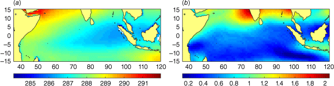
The resulting standard deviation of Tm along with the mean value over the TIO is seen in Fig. A1. From these results, we can obtain the minimum and maximum values that are defined by the authors as the minimum mean minus 1.5 times the standard deviation and the maximum mean plus 1.5 times the standard deviation. The 1.5 scaling is based on experimentation on a few samples with 1.5 standard deviations a safe approximation for the minimum and maximum value. So the minimum Tm value on the altimetry crossover points over the TIO is 283.31 K and the maximum is 288.85 K. Next we calculated the PWV value, using these two extreme ends of Tm and with the maximum value of TWD from the data, which is 42 cm. Note that the maximum TWD value is used so we would not underestimate the approximate deviation. The PWV is 68.36 mm for the maximum and 67.07 mm for the minimum. Since the chosen Tm value in this study is the middle value between the minimum and maximum, this makes the approximate maximum PWV deviation one-half of the difference between the maximum and minimum, which is 0.65 mm.
To determine whether the 0.65-mm PWV deviation is significant, it is compared with the uncertainty of the PWV from the effect of the uncertainty of the TWD. Firstly, the TWD to PWV computation formula (Eqn 1) needs to be resolved. With the Tm value already set to be the middle value (286.08 K), the Π value can be calculated using Eqn 2. Substituting the calculated Π value in Eqn 1, the formula became the following:
which is the TWD to PWV formula used in this study. Now, the effect of the uncertainty of the TWD on the PWV can be estimated. The TWD uncertainty is 0.74 ± 0.15 cm for Jason-1 (Brown et al. 2004). Since the TWD to PWV conversion formula is just a simple scaling, the uncertainty of the PWV is simply the uncertainty of the TWD multiplied by Π as the scaling factor that yields 1.20 ± 0.24 mm. Now we can see that the 0.65-mm PWV deviation due to the use of constant Tm is almost half of the PWV uncertainty and hence can be considered insignificant.
Appendix A2
Monte-Carlo simulation is a method to find the probability distribution of an analysis result by simulating the generation of the analysis several times. Synthetic noise with known parameters is added to the input for each simulation to simulate the random error. The chosen number of times of the conducted simulation is 1000, and a simple convergence test is performed beforehand by computing the significance test 10 times to conclude that using 1000 simulations was sufficient for the test result to be convergent.
The synthetic noise uses a normally distributed random error generated by MATLAB R2017A. The random error is adjusted to have the assumed standard error of the measurement, which is the RMSD generated in Section 3.1, as the standard deviation. A 90% two-tailed significance test is conducted by taking the first 5th percentile of the analysis results as the critical value. Because the original data already contained the random error, adding another synthetic random error would mean that the resulting distribution from the Monte Carlo simulation is exaggerated. Therefore, an adjustment is made to narrow the distribution and obtain the assumed original distribution. This adjustment is done by dividing the standard deviation by √2 because it is assumed that the random error is doubled after adding the synthetic random error. Adding two similar normally distributed variables results in the variance being doubled (Lemons 2002) and so the standard deviation is multiplied by √2. For the composite maps, the critical value should exceed 1.41 mm, which is half of the standard error for the anomaly, to be considered significant.