
Combining a map-based public survey with an estimation of site occupancy to determine the recent and changing distribution of the koala in New South Wales
Daniel Lunney A B , Mathew S. Crowther A C D , Ian Shannon A and Jessica V. Bryant AA Department of Environment and Climate Change (NSW), PO Box 1967, Hurstville, NSW 2220, Australia.
B School of Biological Sciences and Biotechnology, Murdoch University, Murdoch, WA 6150, Australia.
C Institute of Wildlife Research, School of Biological Sciences (A08), University of Sydney, NSW 2006, Australia.
D Corresponding author. Email: mathew.crowther@environment.nsw.gov.au or m.crowther@usyd.edu.au
Wildlife Research 36(3) 262-273 https://doi.org/10.1071/WR08079
Submitted: 22 May 2008 Accepted: 18 February 2009 Published: 15 April 2009
Abstract
The present study demonstrates one solution to a problem faced by managers of species of conservation concern – how to develop broad-scale maps of populations, within known general distribution limits, for the purpose of targeted management action. We aimed to map the current populations of the koala, Phascolarctos cinereus, in New South Wales, Australia. This cryptic animal is widespread, although patchily distributed. It principally occurs on private property, and it can be hard to detect. We combined a map-based mail survey of rural and outer-urban New South Wales with recent developments in estimating site occupancy and species-detection parameters to determine the current (2006) distribution of the koala throughout New South Wales. We were able to define the distribution of koalas in New South Wales at a level commensurate with previous community and field surveys. Comparison with a 1986 survey provided an indication of changes in relative koala density across the state. The 2006 distribution map allows for local and state plans, including the 2008 New South Wales Koala Recovery Plan, to be more effectively implemented. The application of this combined technique can now be extended to a suite of other iconic species or species that are easily recognised by the public.
Introduction
Determining where a species of conservation interest occurs, within its known general distribution limits, is essential for its management; however, mapping a species’ occurrence to a degree that is of practical value for wildlife managers is difficult if the species is widespread and patchily distributed. This difficulty is compounded if the species primarily occurs on private land (Knight 1999) and is cryptic, i.e. its detectability is low (MacKenzie et al. 2003; Wintle et al. 2005). A publicly acceptable and practical way of locating species on private property is to use mail surveys (Lunney et al. 2000a; Lepczyk 2005). These can simultaneously cover a vast area and provide a snap-shot of a species’ distribution (McCaffrey 2005; Toms and Newson 2006). A limitation is that such surveys are confined to iconic species, i.e. those that are well known and cannot be confused with other species. Australia has a sufficient number of such iconic species of pressing conservation interest to test new approaches to map-based mail surveys designed to accurately map their distribution.
A state-wide koala survey was undertaken in New South Wales (NSW) during 1986–87 as part of a national effort (Phillips 1990; Reed et al. 1990). This survey asked residents whether they had seen koalas in their area, the locations of these sightings (without a map, but with addresses to locate the property via The Gazetteer) and whether they thought koala numbers were changing in their area. The survey revealed that the koala had substantially declined in distribution since European settlement. At that time, we hypothesised that there would be further declines of koala populations across its range without better habitat-protection practices on private lands (Reed et al. 1990). In 1992, the koala became listed as Vulnerable in NSW. A series of local studies from 1990 found that koalas mainly inhabit private lands, and that some populations had become extinct or were declining rapidly (Lunney et al. 2002a, 2002b, 2007). Koalas are obligate folivores that depend on selected species of Eucalyptus that grow on fertile soils (Moore et al. 2004), which typically occur on private lands (Pressey et al. 2002). During the preparation of the NSW Koala Recovery Plan (DECC 2008), the need for a new state-wide survey was identified, which then prompted the present 2006 study. In doing so, it also provided us with an opportunity to apply new statistical procedures for estimating site occupancy in combination with a map-based public survey, the only suitable technique for determining the distribution of a species across an area as large as NSW. The koala’s public image, combined with formal national support for its conservation (e.g. ANZECC 1998), made it an ideal subject to test novel survey techniques and analyses.
The 1986–87 koala survey consisted of a small card with basic questions, distributed throughout NSW with a reply-paid return through Australia Post (Reed et al. 1990). Subsequently, more localised surveys included colour maps and requested location records of other iconic species. These proved to be successful in gathering further information, particularly spatially explicit data (e.g. Lunney et al. 1997, 2000a, 2000b; Lunney and Matthews 2001). The simultaneous collection of data for other species enabled us to design a state-wide koala survey to estimate both detection probability and the probability of occurrence. The koala is largely nocturnal and spends the daylight hours often concealed in the tree canopy, giving it a low probability of detection. Assessing the presence or absence of a species when it is often undetected requires different methods from estimating numbers (MacKenzie and Nichols 2004; Joseph et al. 2006; Rhodes et al. 2006a). It is relevant to estimate the number of repeat surveys needed to be reasonably certain that a species is absent (Wintle et al. 2005), as well as to estimate detection probabilities where variation in sampling effort is unavoidable and the estimation of the probability of presence can be confounded by detection probability (MacKenzie et al. 2003).
The primary aim of the present study was to determine the distribution of the koala (Phascolarctos cinereus) in NSW, by using a public survey and applying new statistical models to move from a literal map to one that defines distribution in terms of the likelihood of occupancy. In doing so, we aimed to provide wildlife managers, land-use planners and community organisations with a reliable distribution map for the koala which can be used to support research and conservation programs, such as those identified in the NSW Koala Recovery Plan (DECC 2008). The second aim was to evaluate the effectiveness of combining public survey techniques, in this case with a user-friendly map, with recent developments in estimating site occupancy and species-detection parameters. The third aim was to compare the current distribution with one carried out in 1986–87, to identify any major changes in koala distribution.
Materials and methods
The 2006 study design
The 2006 survey was designed to obtain spatially explicit data on the presence or absence of koalas across the state of NSW (and the Australian Capital Territory, which lies wholly within NSW), Australia (Fig. 1). We used a postal survey of people living outside the major urban areas in NSW to obtain sufficiently accurate animal-sighting data to enable us to establish presence or absence of a species at a local level. We used a design modified from MacKenzie et al. (2006), which depends on several repeat observations at a site, and associated covariates, rather than the approach employed by Dillman (2007), which requires a high response rate if the researcher is to assess the knowledge, or the trends in attitude, in a community. There are recognised limitations to the questionnaire approach (e.g. White et al. 2005), including demographic and socio-political biases in the respondents and biases owing to low return rates (Dillman 2007). However, because our aim was to locate koalas, not estimate the extent of community information or attitudes about wildlife, or demographic characteristics of the human population in relation to knowledge or attitude, these issues did not affect the information used for determining koala distribution. Our survey design aimed to maximise the area of NSW covered, not to sample the human population. Hence, we did not sample Sydney, which, although having many people, covers only a small proportion of NSW. We also could not extensively sample areas of very low human populations (e.g. remote arid and semiarid areas) because of the vast distances and limited postal coverage in these areas. As we had been advised by Australia Post to expect a low return rate, which was consistent with our findings from previous local public surveys seeking detailed, map-based wildlife information, we increased the number of survey forms distributed to be assured of enough returns to undertake the analytical procedures of MacKenzie et al. (2006). In fact, to be confident that we would have sufficient map-based records per 10-km grid square to fulfil statistical requirements for the procedures of MacKenzie et al. (2006), we sent a survey form to a quarter of all residences in rural NSW.
|
We used Australia Post’s unaddressed mail system (i.e. mail delivered without individual addresses) to sample the community across rural and peri-urban (urban fringe) NSW, at a cost of $A0.12–$A0.14 per form dispatched and $A0.40 per return. For delivery purposes, Australia Post divides the State into postcodes, which are postal-delivery zones that vary in area within the state, e.g. Gunnedah is 3837 km2 and Port Stephens is 306 km2. These were the lowest-level identifier that we used during the delivery process. The form was a large, map-based survey, carefully designed to be easy to use. It was an A2 sheet (420 × 594 mm), consisting of a letter and a simple set of questions (Side A), and a user-friendly, colour map for marking wildlife sightings (Side B). The map depicted towns, roads, rivers, National Parks and State Forests at a scale of 1 : 500 000 for eastern and central NSW, and 1 : 850 000 for western NSW. We used 26 overlapping maps to cover the State. Map boundaries were set so each postcode was entirely within at least one of the maps.
The questionnaire side comprised a letter requesting information on the following 10 widely recognised species (or genera): koala, spotted-tailed quoll (Dasyurus maculatus), platypus (Ornithorhynchus anatinus), short-beaked echidna (Tachyglossus aculeatus), brushtail possum (three Trichosurus spp.), common wombat (Vombatus ursinus), wild dog/dingo (Canis lupus familiaris/dingo), red fox (Vulpes vulpes), deer (any species) and cane toad (Bufo marinus). We asked respondents to mark on the map the locations where they had seen each species, differentiating between recent sightings (within the last 2 years) and previous sightings (before the last 2 years). We used only recent sightings for analysis. Most maps allowed a resolution of 1 km for the sightings. The additional information sought was in a simple table, asking ‘yes/no’ as to whether each of the 10 species was present. The questionnaire also asked whether, in the respondent’s view, the density of each species had increased, decreased or stayed the same, and whether the species was a pest in their area. However, because these answers reflect attitudes, and hence different forms of analysis and interpretation (e.g. Dillman 2007), they will be presented elsewhere (D. Lunney, M. S. Crowther, I. Shannon and J. V. Bryant, unpubl. data). There were two additional koala questions (health and presence of young); we also asked how long (in years) the respondent had been living at that address. As optional questions, we asked for the name, age and address of the respondent, whether the respondent was male or female, and whether we may contact the respondent for extra information. The names of the authors and postal address of the Department of Environment and Conservation NSW (now Department of Environment and Climate Change NSW) were given to enable respondents to ask for more information. There were also instructions on how to fill in the map. Both the A and B sides of the survey form can be seen in Lunney et al. (2009a).
In May 2006, we sent out 213 685 survey forms across the state, accompanied by considerable publicity and a phone number to call for questions and media enquiries. We excluded business addresses and most addresses in the high urban concentrations of the Australian Capital Territory, Newcastle, Wollongong and Sydney. We did, however, include Campbelltown, on the outskirts of Sydney, near where the first koala seen by Europeans was discovered 10 years after the British settlement of Australia (Lunney et al. 2009b). We selected the total postal service within each postcode area if feasible and, where not possible, we selected the components of the total service in the following order of preference: (a) roadside mail boxes; (b) street addresses; (c) counter addresses and (d) post office boxes. We also selected more areas of low density of human population in the west of the state to ensure all areas were represented. The allocation procedure produced a threshold level of 473 surveys delivered per postcode, i.e. all postcodes containing up to 473 delivery points were used. Six postcodes above that address limit had all roadside mail boxes and street addresses sampled, because they had been sampled in previous community surveys (Lunney et al. 1996, 1997, 1998, 2004). In total, we selected 278 postcode areas in NSW. To enhance the return rate, we included a postage-paid return envelope. We analysed forms that were returned through to the end of June 2006, giving us a snapshot of current (2004–06) koala distribution across NSW.
Probable density of koala presence
After the forms were returned through the post, we converted the locations of koalas, and other wildlife species, marked on the maps to Lambert’s Projection references and plotted them with ArcGIS 9.0 (ESRI 2007). We projected a 10-km2 grid across NSW for estimating the average occupancy for the koala. At this scale, previous studies of koala distribution have indicated that the effects of spatial autocorrelation are minimal at distances greater than 8 km (McAlpine et al. 2006a, 2006b). Each 10-km grid square was divided into 16, 2.5-km subgrids (i.e. 625 ha) or sites (following the terminology of MacKenzie et al. 2006). For each site, we counted the number of respondents reporting koala presence as well as the number reporting the other nine wildlife species. The reported wildlife sightings of each respondent at each site represented one koala-detection survey (again following the terminology of MacKenzie et al. 2006).
As identified by MacKenzie et al. (2002, 2005, 2006), a major complication in presence/absence studies occurs when a species is present but not detected. The basic model to estimate koala presence (ψ), and the probability of detecting koalas that are present (p) at a site, used the likelihood, given the number of koala and other wildlife sightings:
where ψ is the (unobserved) probability of a koala being present at a site in the bioregion, p is the probability of a koala being detected given that a koala is actually present at a site, Ns is the total number of respondents who reported wildlife at a site, Ks is the total number of respondents who reported koalas at each site, and nCk is the binomial coefficient of k items out of n.
We carried out the analysis for each of the interim biogeographical regions for Australia bioregions (Thackway and Creswell 1995) that occur in NSW, so that there was a species-specific calculation of ψ across each bioregion. This regionalisation of the analysis also improved the estimation of the probability of detection (p), as the characteristics of the different bioregions influenced the chance of detecting koalas.
To further improve the estimation of the probability of a koala being detected (p), the basic model above was augmented by adding the respondent-specific covariates of respondent’s sex and residency (length of time in years that respondent had lived in the area) via a logistic link, following the methods of MacKenzie et al. (2003, 2006), as follows:

To improve the estimation of koala presence at the site level, site-specific environmental covariates were used via a logistic link, as follows:

The parameters (ψ0, ψ1, ψ2, …, and β0, β1, β2) were determined as the values of these parameters that jointly maximised the likelihood equation. The values of the environmental site-specific covariates and ψ0, ψ1, ψ2, … then determined ψ. Likewise, the values of respondent-specific covariates and β0, β1 and β2 then determined p.
We also determined the environmental site-specific covariates to gain a better estimate of the occupancy of a koala at each site (MacKenzie et al. 2003, 2006). These served primarily to remove sites that had few wildlife sightings, and had environmental characteristics that were unlikely to be occupied by koalas. We used the following site-specific environmental covariates: we estimated the mean maximum temperature and annual precipitation for each grid square by using the program BIOCLIM within the ANUCLIM package (Busby 1991; Crowther 2002). Climate data were derived from continent-wide surfaces of monthly mean minimum and maximum temperatures and 19 regional surfaces for monthly precipitation (Williams and Busby 1991). BIOCLIM uses Laplacian smoothing splines to incorporate mathematical surfaces to a network of existing meteorological data (Hutchinson and Bischof 1983; Hutchinson et al. 1984). We used the GEODATA 9 Second Digital Elevation Model (DEM-9S) Version 2 of Australia (http://www.agso.gov.au/meta/ANZCW0703005624.html) to calculate the mean elevation for each 10-km grid square with ArcGIS 9.0 (ESRI 2007). Human population and its associated habitat modification, transport and dog ownership are acknowledged as having an impact on koala habitat and koala survival (Lunney et al. 2002b, 2007). We incorporated the data on the human-population density from the Australian 2001 census, using collector district totals proportionally spread over each grid cell, in the analyses. We classified soil layers into four fertility levels, and used the presence of a Soil Fertility Class 3 as a binary covariate because this class showed the most variation between the presence and absence of koalas. Also, we treated the presence of roads, rivers and streams as binary covariates, within each 10-km grid, because their presence or absence reflects the presence or absence of koalas and other wildlife species.
We used the SAS procedure NLIN (http://support.sas.com/onlinedoc/913/getDoc/en/statug.hlp/nlin_index.htm) to derive the maximum likelihood estimates and their variances.
By using those estimates, we defined the probability of a koala being present at each site as:
That is, if a koala was reported, we set the probability to 1; otherwise, the probability depended on ψ, p and the number of sightings of other species. For each 10-km2 grid, the average occupancy was calculated as the sum of the 16 probabilities of koalas being present, divided by 16. A value of 1.0 arose where koalas were reported at all 16 sites. Values close to zero reflect a large number of records of other wildlife, and few or no koala sightings. Higher values reflect increasing support by the data for koala presence throughout the grid square. Because both the fox and the echidna are known to be widespread, as are several other species, at least 1 of the 10 species was predicted to occur in every grid square (e.g. van Dyck and Strahan 2008). Thus, if no wildlife sighting of any species was detected in a 10-km2 grid square, that grid square was deemed not to have been surveyed.
Distance from home
We asked respondents to mark the location of their residence on the map. This provided us with an indication of whether the records were accurate for location. We assumed that the respondent would know the location of their house on the user-friendly map that showed roads and towns; hence, koala sightings near the house would be more likely accurate for location. This analysis was also used to provide a measure of the dispersion patterns of individual respondents’ wildlife records and their proximity to the respondent’s house.
Sufficient information
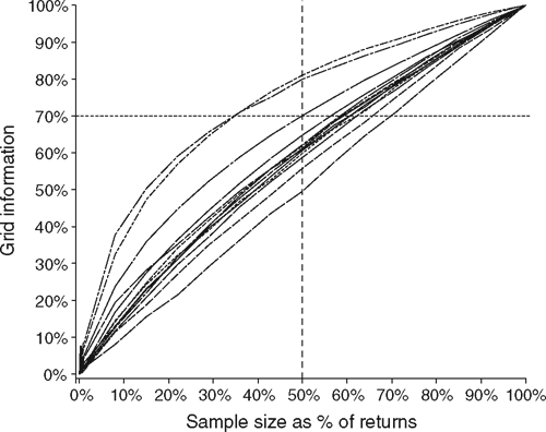
To test whether the intensity of the survey was adequate, we plotted a cumulative number of new koala locations against a cumulative number of forms returned. For each of the 26 map sheets, we constructed curves to indicate whether we sampled intensively enough to capture the distribution of the koala. A steep curve indicated that we were still collecting new koala locations to the end of the survey. In contrast, a curve that flattened indicated that no or little new information was being added with additional returns. As the survey distribution assigned all the respondents’ addresses, in whole postcodes, to the same map, all wildlife data in a postcode area occurred on one map.
We calculated the mean information content α(φ) as the proportion of information (koala locations) in subsamples of the total returns on each map, for subsample sizes φ ranging from 5 to 95%. The definition of the function α(φ) constrains it to go through the points α(0) = 0 and α(1) = 1.
Estimating differences in koala distribution between the 1986 and 2006 surveys
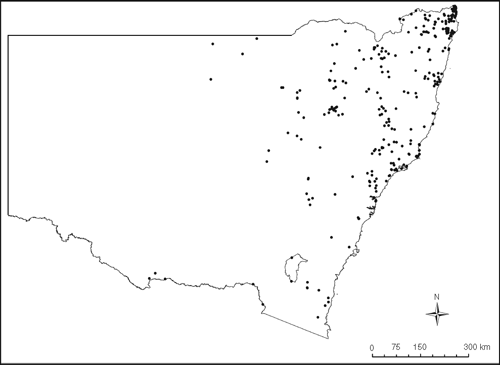
We compared the data for the 1986 (Fig. 2) and 2006 community surveys by basing the comparisons on equal measures, i.e. by resampling the 2006 results to standardise them to the 1986 sampling intensity. This enabled us to detect significant changes in the relative koala density. The response rate in 2006 was significantly greater than that in 1986, i.e. 16 526 compared with 890 respectively. Therefore, we estimated the differences in the number of koala sightings in each 10-km grid cell by applying the response rate of 1986 onto the 2006 dataset. Because there were substantially more 2006 records than there were 1986 records, there were many such possible combinations of the 2006 dataset, sampled at the 1986 response rate. Hence, we resampled the 2006 data to provide us both with 1986-comparable data and to determine estimates of variability of survey responses at the 10-km grid level. With a resampling effort of 10 000, most grid cells had sufficient 2006 samples to estimate the empirical distribution of the difference in koala spread between 1986 and 2006. From the distributions (at the grid-cell level), we calculated a 95% confidence interval for the difference.
|
Results
The 2006 survey received 16 526 replies, a return rate of 7.7%, which greatly exceeds the usual return rate of less than 2% for commercial surveys and promotions (Australia Post, pers. comm., May 2006). The values for each step in the distribution and return of forms show that of those who replied, 11 087 had a map-based location of at least one of the 10 animal species (Table 1). Of the 51 469 animal records, i.e. ‘sightings’ pinpointed on the maps, there were 4904 koala sightings on 3110 forms, i.e. 1.58 koalas per form with a koala sighting. In round figures, of those who were sent a survey, 1/8 responded; 2/3 of the returned survey forms had animal locations, 1/4 of the returned forms had koala locations and 1/10 of the total number of animal sightings were of koalas.

|
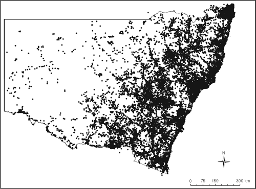
The distribution of wildlife records covered the eastern half of NSW. There were gaps in the west and central west of NSW, and along the Great Dividing Range (Fig. 3). These gaps reflected gaps in the locations of respondents’ houses (Fig. 4).
|
|
There was a variable rate of accumulation of information on koala locations for the increasing number of surveys returned (Fig. 5). The three map sheets covering the north-eastern part of the state, where koalas were principally located, showed a high rate of return, e.g. 70% of the information by 50% of the returns. The other koala curves show a lower rate, and these map sheets were in those areas where koalas were scarce. After the entry of 16 526 surveys, we were still gaining more information on koala distribution in most of the 26 areas defined by the map sheets (Fig. 5). This is consistent with the reporting rate expected for rare species, i.e. in most map sheets koalas were rare, as well as being the expected rate of reporting for those parts of the state where the species is more common, in this case in north-eastern NSW.
|
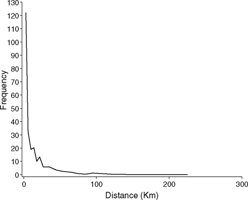
Most wildlife sightings were within 2.5 km of respondents’ residences (Fig. 6), with almost all records falling within 20 km. Animal reports more than 10 km from a dwelling were relatively scarce. The same decline of records was common across all species, despite the squared increase in area, and hence potential koala habitat, with distance from a fixed point. Because of the respondents’ likely familiarity with the locality near to their homes, we consider that the animal locations were well within the accuracy required for placement into a 2.5-km grid.
|
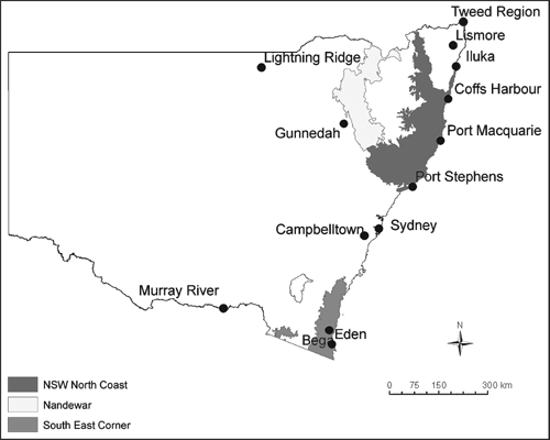
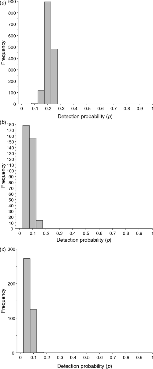
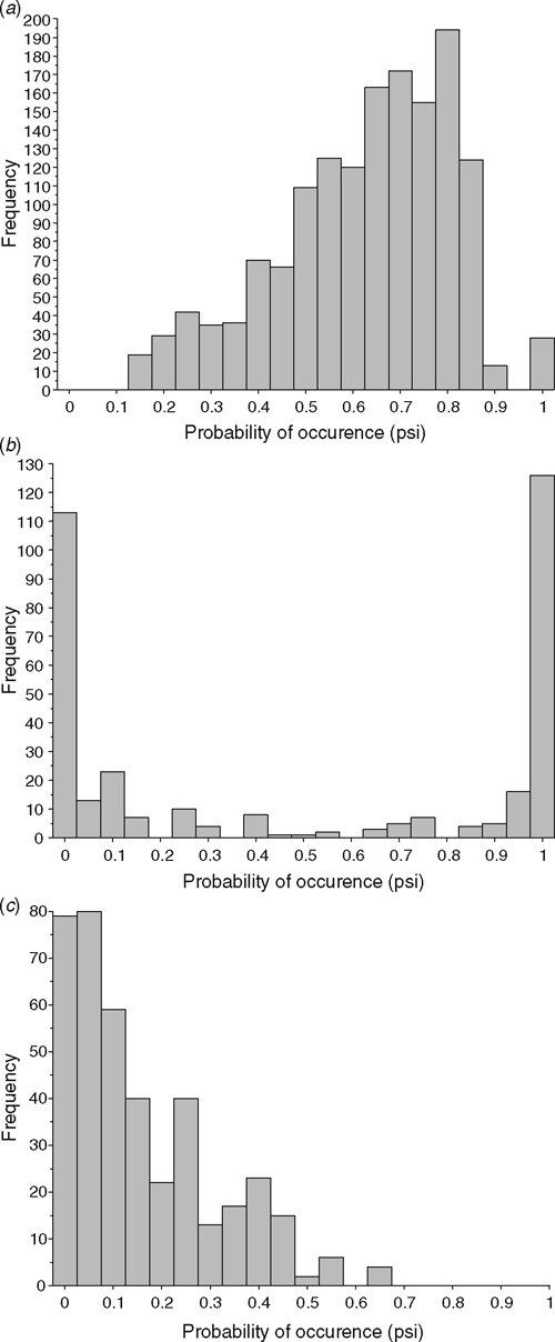
There was a great variation in the probabilities of both detectability and occupancy among different bioregions; hence, a decision was made to apply bioregion-specific estimates of detectability and occupancy. For the purposes of comparison, only the North Coast NSW, Nandewar and South-east Corner bioregions are given for analysis (Fig. 1). In the North Coast NSW bioregion, detectability was higher than in other bioregions, ranging from 0.1 to 0.3 (Fig. 7a), reflecting the higher number of respondents in that area. Detectability was lower in the Nandewar and South-east Corner bioregions than in the North Coast NSW bioregion (Fig. 7b, c). The comparisons of occupancy showed a different pattern, with a spread of relatively high occupancies in the North Coast NSW bioregion (Fig. 8a). There was a bimodal distribution of occupancies in the Nandewar bioregion, reflecting the clustering of koalas around Gunnedah (Fig. 8b). In the South-east Corner, there were lower occupancies than in the North Coast NSW, reflecting fewer recent koala records (Fig. 8c).
|
|
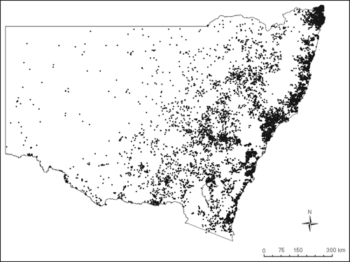
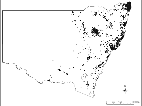
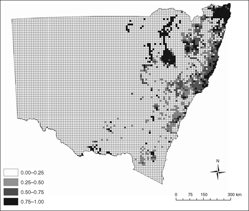
The records of koalas were unconnected across much of the range, with clusters evident along the northern half of the coast, and a major cluster in the northern region of the state, west of the Great Dividing Range (Fig. 9). The final map, which is the outcome of the application of the estimates of site occupancy and species-detection parameters, is accurate in that it shows where koalas were known to exist in 2004–06 (Fig. 10). Areas where there was a very high likelihood of koala presence include the Tweed region of far-northern coastal NSW, the areas surrounding Coffs Harbour and Port Stephens of mid–north coast of NSW, and the area surrounding Gunnedah, north-western NSW. The western extremities of areas of high likelihood of koala presence include the areas surrounding Lightning Ridge, and some locations along the Murray River. In contrast, the far-southern coast and the far-western region of NSW have very low likelihoods of koala presence (Fig. 10).
|
|
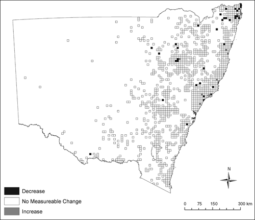
Comparison between the 1986 and 2006 surveys showed how the concentrations of koalas have changed (Fig. 11). This comparison cannot show absolute changes in koala numbers, rather it shows those areas of the state where koalas have decreased or increased faster than in the rest of the state. Specifically, it highlights only a few grid squares, around Gunnedah in north-western NSW and some areas on the northern coast of NSW, that showed a significant increase in koala concentration. For most of the grids, the data did not show a statistically significant difference in koala presence/absence. This lack of detected differences would be due to both the low level of statistical power (determined by the size of the historical 1986 dataset) for some grid cells, as well as there being no real differences between the time periods in other grid cells. Areas showing decreases in relative koala density were often adjacent to the areas of increase in far-northern NSW and in some grid squares to the south-west of Gunnedah (Fig. 11).
|
Discussion
The success of this novel combination of methods (estimates of site occupancy and species detectability applied to spatially explicit data from public survey) has demonstrated that public surveys can provide information on species distributions on private lands. These lands are the habitat of many threatened species, as well as emerging pests (Knight 1999; Norton 2000; Lunney and Matthews 2001). Although public-survey methods are utilised in species biology (e.g. Lunney et al. 2000a; Lepczyk 2005), and there are studies estimating species presence when detectability is variable (Bailey et al. 2004), we know of no other study that has combined these techniques. We are confident that the survey encompassed the koala’s range because the locations of the koalas were a subset of the locations of all 10 species of wildlife surveyed, i.e. there were many more 10-km2 grid cells with wildlife other than koalas. Determining the distribution of a widespread species is difficult, particularly when it is patchily distributed, is cryptic and inhabits private lands, as is the case with the koala. Estimating the detection probability across a survey area provides a valuable tool in such studies (MacKenzie et al. 2006).
We are mindful of the shortcomings of wildlife records that are based on human observations. This applies particularly to the western half of NSW and the Great Dividing Range, large sections of which are neither farmed nor occupied. The western third of the state is arid or semiarid, with a low density of human population, where koalas are restricted to riparian areas of some major, although intermittently, flowing rivers (Reed et al. 1990). However, the scale of the 2006 survey, the size of the response and the high quality and quantity of spatially explicit data obtained by the use of a large, user-friendly map, demonstrate that compiling a comprehensive and reliable distribution of the koala in NSW is possible by using unaddressed mail. In particular, it has confirmed the value of this non-intrusive method for obtaining wildlife-distribution data from private lands.
The survey covered the rural landscape across a large area of NSW (809 444 km2). Most koala sightings were within the immediate vicinity of respondents’ houses, i.e. were mostly on private land, in rural areas. However, there were sufficient records 10–40 km from residences to enable wildlife locations to be identified in nearby state forests or national parks. The map of locations of all wildlife-survey records (Fig. 3) covers far more ground than the map of respondents’ houses (Fig. 4), particularly in the strip along the Great Dividing Range, an area largely devoted to forests and parks (Pressey et al. 1996, 2002). This survey technique has great strengths where people live, and where the population density is sufficiently high to support a survey.
Ideally, the information curves plotting the number of wildlife locations recorded against the number of survey returns would approach a horizontal asymptote. The curves did record a declining mean rate of new information per return for the common species, e.g. the red fox (D. Lunney, M. S. Crowther, I. Shannon and J. V. Bryant, unpubl. data). These curves allowed us to conclude that we did not significantly undersample to preclude adequately encompassing the rarer species, such as the koala. Further, where the koala was most commonly found, the curves were flattening, with 70% of the information by 50% of the returns. The resulting maps of koala distribution can therefore be considered to be reliable, especially because detection rates were accounted for. We note that we were the first to examine the intensity of any planned postal wildlife survey on such a large scale. We have now provided a gauge of the effort necessary to achieve a reliable and repeatable result. However, we would not recommend annual monitoring by this method at this effort because of the cost. Targeted local studies would be the next step.
Maps of wildlife-location records, depicted as large dots, are potentially misleading. In Fig. 9, each point is one koala-location record. On the far-southern coast, there appears to be a reasonable smattering of records, whereas on the far-northern coast there is a noticeably thicker cluster of records. A direct comparison between these two locations points to a higher density in the north than the south, although the degree of difference is concealed by the size of the markers showing each location record. A greater appreciation of the interpretation of species distribution emerges from a comparison between the map of koala records (Fig. 9) and the map of the average occupancy values for the koala (Fig. 10). This final map of estimated koala presence is of much greater value to field managers and planners than the precursor map of koala locations. It gives the index of species presence in a locality generally, and is related to the likelihood that koalas are present in a randomly chosen 625-ha area, i.e. 10 km2. It also allows others to appreciate how likely, with a given level of probability of detection, it would be to detect a koala if a local search were to be conducted. The far-southern coast was identified in 2006 as being largely bereft of koalas, a point consistent with the scant records found during past surveys and an examination of the historical record (Lunney and Leary 1988; Lunney et al. 1997). In other words, koalas are present, although locally rare. However, the koala in the Eden region remains of great local conservation interest and, in the debate in the media over woodchipping, it has been the most frequently mentioned wildlife species (Lunney 2005). In contrast, the northern coast of NSW and the area around Gunnedah on the Liverpool Plains, west of the Great Dividing Range, are recognised locally as carrying important koala populations (Smith 2004; Lunney et al. 2007). The next step would be to confirm koala-sighting records with another series of ‘on-ground’ field surveys, such as those used by Lunney et al. (1998) and those identified as targets in the NSW Koala Recovery Plan (DECC 2008). Studies have already commenced in the Gunnedah region of NSW (D. Lunney, M. S. Crowther, I. Shannon and J. V. Bryant, unpubl. data), where the koala population has expanded against the state trend. Of particular focus in the Gunnedah study is the use that the koalas are making of the major tree-planting programs of the 1990s, and whether these restoration programs are the primary reason for the increase.
The use of public survey depends on several criteria that we ensured we satisfied before undertaking this enterprise. The first was selecting only easily recognised, iconic animals, such as the koala, red fox and echidna. Except for the cane toad, all are ubiquitous and widespread species/genera that share an extensive distribution from the coast to the arid zone in NSW. They have no congeners in Australia, so there is no ambiguity about their identification. The second criterion was to select species that are likely to occur on private lands. The third was to use a map where respondents could readily show the location of their residence, to help them accurately indicate the locations of their sightings. The fourth criterion was to select species that live where people live; the eastern half of NSW has been shown by the present study to fit that category, and whereas the method is weaker in the arid zone with fewer people, it would be of great value for studies of urban wildlife (e.g. Lunney and Burgin 2004; Adams et al. 2006).
By resampling the 2006 koala-survey data (Fig. 9), we were able to identify the areas that reported an increase or decrease in the relative density of koala sightings since 1986 (Fig. 11). The only areas that reported an increase in the relative density of koala sightings were on the northern and mid–northern coast of NSW, and in the immediate vicinity of Gunnedah, an area that undertook tree plantings in the 1990s, and had been recording more sightings of koalas (Smith 1992; S. Rhind, M. Ellis, M. Smith and D. Lunney, DECC, unpubl. data). This is indicated by the higher concentration of sightings surrounding Gunnedah in the 2006 survey (Fig. 9) than that in the 1986 survey (Fig. 2). We note that these increases were adjacent to grid squares reporting relative decreases in koala sightings to the south-west of Gunnedah. Most areas did not report a relative change in koala sightings, which may be due to the small number of responses in many of these squares, or the areas not having had (and still not having) substantial koala numbers in the past 20 years, particularly on the far-southern coast and western NSW. The 20-year comparison also revealed that the 1986 map of Reed et al. (1990), as shown in Fig. 2, was a reasonable estimation of the distribution of the koala in NSW. Hence, the detailed programs that were based on this state-wide portrait were not misplaced. It gives us greater confidence that the next generation of policies and programs, such as those in the NSW Koala Recovery Plan (DECC 2008), will be addressing contemporary issues in koala biology and conservation.
Most of the grid squares reporting decreases in relative koala density were in the north-east of NSW, the identified stronghold of koala populations in the 1986–87 survey (Reed et al. 1990), and now an area of rapid growth of human population (NSW Department of Planning 2006a, 2006b). These areas fell behind the general trend across NSW during the 20-year period since the 1986 survey. We consider that the rapidly increasing human population, with its increase in associated threats of habitat fragmentation, dogs and motor vehicles, has led to declines in the koala population in this area relative to the rest of the state. Some koala populations in northern NSW have already been reported as becoming locally extinct (Lunney et al. 2002b), or declining (Lunney et al. 2007; Matthews et al. 2007). We predict that populations will continue to decline as the human population continues to increase, unless specific management actions are taken (DECC 2008).
Current conservation programs are already utilising our final distribution map, such as in the efficient implementation of the NSW Koala Recovery Plan (DECC 2008), and the map will form part of the current redrafting of the National Koala Conservation Strategy (ANZECC 1998). The location data are also publicly available on DECC’s Atlas of NSW Wildlife. Access to such data is particularly important where the costs of implementation are high, e.g. the estimated costs for implementation of the NSW Koala Recovery Plan are $A1 230 000, as stated at the official launch of the Recovery Plan on 30 November 2008. The map also serves as a springboard for further research, such as monitoring and interpreting trends in the status of the koala, the impacts of climate change, undertaking local population studies, and examining the contributions of planning and restoration programs to the maintenance of local koala populations. Recent examples are the research by Rhodes et al. (2006b, 2008), McAlpine et al. (2006a, 2006b, 2008) and Januchowski et al. (2008), which used the koala as a model species to examine broad ecological issues where there is a management imperative.
Conclusions
Wildlife managers, land-use planners and community organisations now have a set of distribution maps which can be used to fulfil the aims of the NSW Koala Recovery Plan (DECC 2008) and related research and conservation programs. Although public surveys have regularly been used in applied ecology and natural-resources studies (e.g. Lunney et al. 2000a; Lepczyk 2005), there have been methodological advances in recent years (White et al. 2005). The combination of public survey, which is map-based, with the estimation of site occupancy has wide application where conservation actions on private land, and community participation, will be integral to the success of proposed planning decisions or wildlife-management programs. The practical application of this technique enhances the capacity of spatially explicit public surveys to provide a rigorous and repeatable basis for ecological studies, such as the NSW state government’s current emphasis on monitoring, evaluation and reporting (MER) or the Commonwealth’s MERI (where the ‘I’ stands for improvement). Involving the community in the research phase of an ecological study, such as determining the distribution of koalas, encourages the community to participate in implementing conservation actions (Lunney et al. 2000a; DECC 2008). Because these actions will principally apply to private lands, it is crucial to have community support. This principle applies to a wide suite of species that are of public concern, including threatened species and pest species, on private lands. Conserving koala populations in NSW and managing the associated threats and planning options are among the immediate positive outcomes of this approach (e.g. McAlpine et al. 2007; DECC 2008).
Acknowledgements
We thank the following DECC NSW staff: S. Smith for funding; M. Stephens, R. Avery and R. Ruffio for map design and data-entry formatting, P. Sherratt for design of survey sheet; C. Togher and E. Knowles for GIS assistance; S. Rhind for her focus on Gunnedah, and D. Plowman for assistance with the Atlas; a competent data-entry team; A. House and Know-Ware for assistance; J. Baker for organisational support, and I. Dunn, M. Ellis, D. MacKenzie, C. McAlpine, C. Moon and J. Rhodes for their critical comments on the manuscript. We also acknowledge the help the anonymous reviewers and the editor, A. Taylor, gave to the manuscript.
Bailey, L. L. , Simons, T. R. , and Pollock, K. H. (2004). Estimating site occupancy and species detection probability parameters for terrestrial salamanders. Ecological Applications 14, 692–702.
| Crossref | GoogleScholarGoogle Scholar |
Crowther, M. S. (2002). Distributions of species of the Antechinus stuartii–A. flavipes complex as predicted by bioclimatic modelling. Australian Journal of Zoology 50, 77–91.
| Crossref | GoogleScholarGoogle Scholar |
Hutchinson, M. F. , and Bischof, R. J. (1983). A new method for estimating the spatial distribution of mean seasonal and annual rainfall as applied to the Hunter Valley, New South Wales. Australian Meteorological Magazine 31, 179–184.
Lunney, D. , and Leary, T. (1988). The impact on native mammals of land-use changes and exotic species in the Bega District New South Wales since settlement. Australian Journal of Ecology 14, 67–92.
Lunney, D. , Esson, C. , Moon, C. , Ellis, M. , and Matthews, A. (1997). A community-based survey of the koala, Phascolarctos cinereus in the Eden region of south-east New South Wales. Wildlife Research 24, 111–128.
| Crossref | GoogleScholarGoogle Scholar |
MacKenzie, D. I. , and Nichols, J. D. (2004). Occupancy as a surrogate for abundance estimation. Animal Biodiversity and Conservation 27, 461–467.
Matthews, A. , Lunney, D. , Gresser, S. , and Maitz, W. (2007). Tree use by koalas Phascolarctos cinereus after fire in remnant coastal forest. Wildlife Research 34, 84–93.
| Crossref | GoogleScholarGoogle Scholar |
McAlpine, C. A. , Rhodes, J. R. , Bowen, M. E. , Lunney, D. , Callaghan, J. G. , Mitchell, D. L. , and Possingham, H. P. (2008). Can multiscale models of species’ distribution be generalized from region to region? A case study of the koala. Journal of Applied Ecology 45, 558–567.
| Crossref | GoogleScholarGoogle Scholar |
Norton, D. A. (2000). Conservation biology and private land: shifting the focus. Conservation Biology 14, 1221–1223.
| Crossref | GoogleScholarGoogle Scholar |
Pressey, R. L. , Ferrier, S. , Hager, T. C. , Woods, C. A. , Tully, S. L. , and Weinman, K. M. (1996). How well protected are the forests of northeastern New South Wales? Analyses of forest environments in relation to tenure, formal protection measures and vulnerability to clearing. Forest Ecology and Management 85, 311–333.
| Crossref | GoogleScholarGoogle Scholar |
Rhodes, J. R. , Tyre, A. J. , Jonzén, N. , McAlpine, C. A. , and Possingham, H. P. (2006a). Optimizing presence-absence surveys for detecting population trends. Journal of Wildlife Management 70, 8–18.
| Crossref | GoogleScholarGoogle Scholar |
Toms, M. P. , and Newson, D. E. (2006). Volunteer surveys as a means of inferring trends in garden mammal populations. Mammal Review 36, 309–317.
| Crossref | GoogleScholarGoogle Scholar |
White, P. C. L. , Jennings, N. V. , Renwick, A. R. , and Barker, N. H. L. (2005). Questionnaires in ecology: a review of past use and recommendations for best practice. Journal of Applied Ecology 42, 421–430.
| Crossref | GoogleScholarGoogle Scholar |

Williams, W. D. , and Busby, J. R. (1991). The geographical distribution of Triops australiensis (Crustacea: Notostraca) in Australia – a biogeoclimatic analysis. Hydrobiologia 212, 235–240.
| Crossref | GoogleScholarGoogle Scholar |
Wintle, B. A. , Kavanagh, R. P. , McCarthy, M. A. , and Burgman, M. A. (2005). Estimating and dealing with detectability in occupancy surveys for forest owls and arboreal marsupials. Journal of Wildlife Management 69, 905–917.
| Crossref | GoogleScholarGoogle Scholar |