

Electronic Wavefunction Tiles
Yu Liu A , Terry J. Frankcombe B and Timothy W. Schmidt A C
A C
A ARC Centre of Excellence in Exciton Science, School of Chemistry, UNSW Sydney, NSW 2052, Australia.
B School of Science, UNSW Canberra, ACT 2600, Australia.
C Corresponding author. Email: timothy.schmidt@unsw.edu.au
Australian Journal of Chemistry 73(8) 757-766 https://doi.org/10.1071/CH19517
Submitted: 15 October 2019 Accepted: 25 November 2019 Published: 6 May 2020
Journal Compilation © CSIRO 2020 Open Access CC BY-NC-ND
Abstract
We review the pre-quantum theories of electronic structure of Lewis and Langmuir, and how this relates to the post-quantum double-quartet theory of Linnett. Linnett’s ideas are put on a firm theoretical footing through the emergence of the wavefunction tile: The 3N-dimensional repeating structure of the N-electron wavefunction. Wavefunction tiles calculated by the dynamic Voronoi Metropolis sampling method are reviewed, and new results are presented for bent bonds of cyclopropane, and electron correlation in Be-O-Be.
Introduction: Lewis, Langmuir, Louis, London, Linus and Linnett
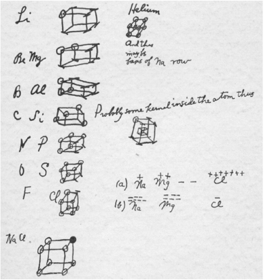
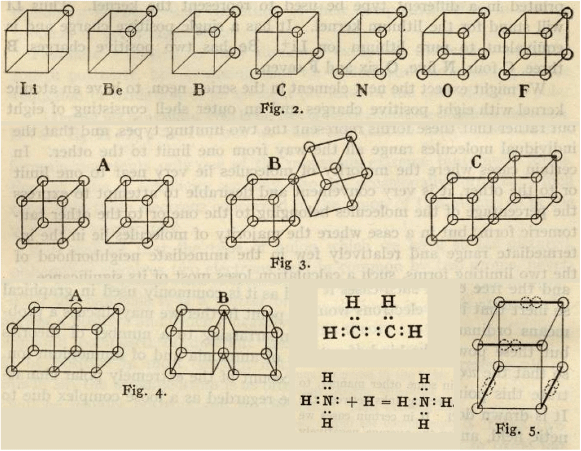
In 1902, Gilbert Lewis wrote down the beginnings of what would later become the familiar ‘octet rule’ of chemistry (see Fig. 1).[1] He imagined that electrons were fixed to the vertices of a cube, and that the vertices were sequentially filled in as one moved across the periodic table. The concept of core electrons was accounted for by cubes-within-cubes, written by Lewis as ‘Probably some kernel inside the atom thus’. The tetrahedral geometry of carbon could be accounted for, to some extent, by the way that the vertices were occupied.
|
In 1916 Lewis published his seminal paper, in which he laid out the basis for much of the pictorial description of chemical structure still used today. As shown in Fig. 2, Lewis rationalised the covalent bond as the sharing of two electrons, which we would later understand as having opposing spins. He conceded that the cubical view of atoms was unable to reconcile the free rotation of single bonds, nor the triple bond, and thus proposed a variation in which the electrons were located at the vertices of a tetrahedron:
‘… two tetraheda, attached by one, two or three corners of each, represent respectively the single, the double and the triple bond. In the first case one pair of electrons is held in common by the two atoms, in the second case two such pairs, in the third case three pairs.’
|
Lewis goes on to state that:
‘The triple bond represents the highest possible degree of union between two atoms’,
a notion that would largely stand the test of time. Finally, Lewis accounted for the colours of various compounds by reasoning that the electrons vibrate about their equilibrium positions.
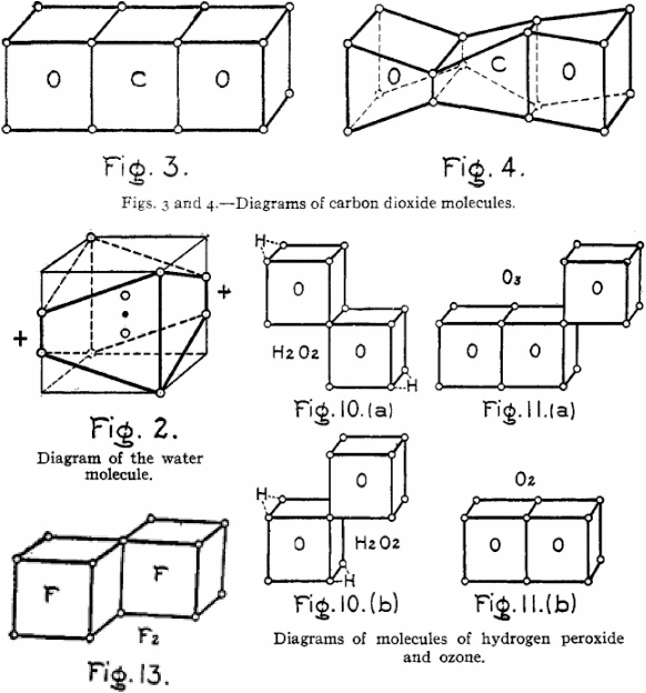
In 1919 Langmuir built upon Lewis’ ideas and proposed structures for a great number of compounds, including ozone (Fig. 3).[3] He proposed structures for water and CO2 which required devations from the cubic atoms model.
|
|
But this was an exciting time for electronic structure theory. Louis de Broglie published the wave-postulate in 1925,[4] and Schrödinger outlined the basis of wave-mechanics in a series of papers in 1926.[5] By 1927 Heitler and London had proposed that a resonance between alternate occupancy of atomic orbitals in H2, by up and down-spin electrons, gave rise to the chemical bond.[6] This is the basis of valence bond theory. Quantum mechanics was on the ascendancy.
Work by Lennard-Jones,[7] Hund,[8] Mulliken,[9] and Hückel[10] established molecular orbital (MO) theory as a rival theory to valence-bond (VB) theory. Due to algorithmic simplicity for computational purposes, MO theory has won out. And, because of its popularity with computational chemists, it has been regarded by many chemists as ‘more correct’. However, as Pauling points out,[11] they are both based on the same concept,
‘… the principle that the correct wave function for a state of a system (such as the normal state) can be expressed as a sum of functions constituting a complete set.’
As such, it does not matter what those functions are.
Linus Pauling laid out his vision in a series of papers entitled ‘The Nature of the Chemical Bond’ in 1931. In the first installment[12] we are introduced to the idea of orbital hybridisation (‘bond eigenfunctions’), which for four electrons lie at the corners of a tetrahedron (Fig. 4).
In 1962, Linnett picked up on the simple theories of Lewis, Langmuir and Pauling and developed his double-quartet theory (DQT).[13,15] This idea is based on the fact that the most probable disposition of four valence electrons of the same spin about an atom is a tetrahedron.[16] The two spin sets are considered separately, and the electronic structures of many molecules are explained in this way. Fig. 5 reproduces double-quartet structures of F2, ethylene, and O2, as redrawn in our first paper.[14] Though not a quantitative theory, DQT forms a bridge between Lewis’ original ideas and chemical observations. For example, the triplet structure of O2 can be seen to separate the two spin sets, thus reducing the electron repulsion energy. This structure may be compared to that drawn by Langmuir (Fig. 3). It was happy chance that one of us (TWS) found Linnett’s book on a shelf in the underground laser laboratory of Prof. John P. Maier in Basel. The structures of Linnett bore a striking resemblence to structures which emerge when attempting to perform quantum Monte Carlo calculations for fermions, without guiding functions.
|
The rivalry between MO and VB theory continues,[17–19] with much of chemistry explained on the basis of VB concepts with local bonds constructed from (hybrid) atomic orbitals, augmented with resonance where necessary, and most quantitative calculations being performed using MOs. It is because most modern calculations generate MOs that many chemists leap to interpret them as somehow real.† Indeed, a case in point is the interpretation of photoelectron spectra which are often (over)-interpreted in terms of molecular orbitals.[20]
The simplest wavefunction which obeys the Pauli exclusion principle (in its crudest form) is a product of one-electron functions, known as the Hartree product.
The Hartree product, where each electron has a corresponding orthogonal one-electron function is the view of wavefunctions that most chemists hold. However, this function does not obey the underlying origin of the Pauli principle, namely that the wavefunction is antisymmetric upon exchange of electrons (fermions).
To achieve this property, a determinant is constructed such that the diagonal of the matrix is the Hartree product. Exchange of any two rows will change the sign of the determinant, and thus the wavefunction itself. The simplest molecules are reasonably well-described in terms of a single-determinant wavefunction. The determinant, named for Slater, is written
The structure of this wavefunction does not resemble the one-electron functions in any way. Indeed, it is invariant to a unitary rotation of the occupied orbitals: Any orthogonal set of linear combinations of the canonical orbitals, which are eigenfunctions of a fictitious one-electron operator, yield the same many-electron wavefunction. But, it is the antisymmetrised wavefunction which has the properties acknowledged by Linnett that keeps four valence electrons of the same spin at an average tetrahedral disposition.
In just one spatial dimension, the ‘two like-spin-particles in a box’ problem illustrates the differences between the (canonical) Hartree product, the Slater determinant, the canonical orbitals, and localised orbitals. In Fig. 6, the two lowest one-particle eigenfunctions are plotted and labelled ‘canonical orbitals’. This is the standard chemists’ view of chemical structure. The two-dimensional function that results from this way of thinking is plotted as a colour map and labelled ‘canonical Hartree product’. However, this wavefunction does not obey the property that the wavefunction changes sign upon exchange of like-spin electrons. The Slater determinant is plotted in Fig. 6 and labelled thus. One can see that this function is indeed antisymmetric, and that it in no way resembles the canonical orbitals. However, it does resemble a ‘jaffle’ – a toasted sandwich with two equivalent halves.

|
The antisymmetrised wavefunction for two like-spin electrons must have two equivalent halves, because for every point (x1, x2), there is a point (x2, x1) with the same magnitude of the wavefunction. The repeating structure of a many-electron wavefunction is the ‘tile’, the subject of this manuscript. Each half of the jaffle is a wavefunction tile. A set of localised orbitals, found by a π/4 rotation of the canonical orbitals, may be multiplied together to obtain a very crude representation of one tile (localised Hartree product), and one can see that the localised orbitals resemble the projections of the tile, R, onto each electron’s dimension,  .
.
It is all well and good to explore the wavefunctions of one-dimensional particles, but how would one visualise the many-electron wavefunction in higher dimensions? One approach is to explore the wavefunction using a Monte Carlo algorithm.
Quantum Monte Carlo
As contemporary undergraduates, TWS and TJF were exposed to the idea of diffusion quantum Monte Carlo‡ (DMC), an intriguing theory which promises to return the ground state energy of a many-body quantum system, including the correlation energy. The trick is that because electrons are fermions, the wavefunction must change sign upon the swap of two electrons of the same spin. But there is no ‘sign’ in DMC, there is only the density of the diffusing ‘walkers’. In order to introduce nodes, armies of walkers can be diffused, with their interpenetration rendered forbidden. The armies need to consist of all like-spin permutations of the ‘principal walker army’, which is the set of walkers under diffusion (and breeding/execution) orders from a random-number generator.
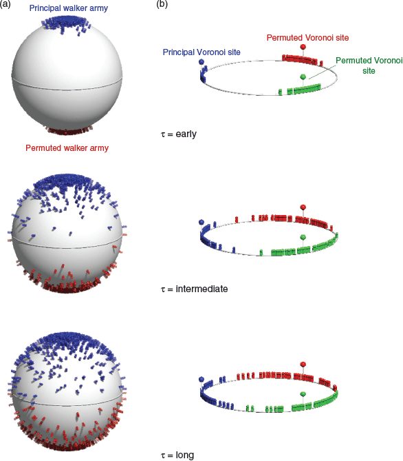
This principle can be illustrated by the toy quantum problem of two like-spins, a and b, on the end of a stick of fixed length (Fig. 7a). The configuration is defined by the orientation of the stick as defined by the vector connecting the origin (stick midpoint) to, say, spin a. As an army of walkers commences at the North pole (θ = 0), it diffuses South, while a ‘ghost’ army representing the permutation a ↔ b diffuses North. For every walker, there is a permuted, antipodean walker. After some (imaginary) time, the armies meet at the equator. As they are prohibited from interpenetrating, the principal walker army remains in the Northern hemisphere and the permuted walker army, representing the negatively-signed part of the wavefunction, remains in the Southern hemisphere. At equilibrium, the walker distribution will represent the spherical harmonic of the pz atomic orbital, which is the J = 1, MJ = 0 rotational wavefunction of ortho-hydrogen – two like-spins (protons) on a stick! Because the distribution in the Southern hemisphere depends solely on that in the Northern hemisphere, all of the information of the system is contained in the latter, and the former can be regenerated from the latter. This is the basis of the ‘wavefunction tile’, the repeating unit of the wavefunction which is the subject of the present manuscript. It is important to note that the walkers define the tile. The positions of the walkers define the node (for instance, as a Voronoi diagram of the walker ensemble, including permuted walkers).
In the case of two like-spins at a fixed distance, the starting point of the problem will determine the outcome in the limit of infinite walkers. Starting at the North pole results in the node appearing at the equator. In the absence of a potential, starting the ensemble anywhere else will result in the node appearing on a Great Circle 90° from the starting point. Statistical fluctuations will cause deviations. The non-uniqueness of the solution is on account of the threefold degeneracy of the J = 1 state: MJ = 0, ±1. Because the solutions are real, the MJ = ±1 solutions will be obtained as real linear combinations, analogous to the chemist’s px and py orbitals, which are not eigenfunctions of the lz operator.
|
The Voronoi Diagram
Once three like-spins interact, there becomes the possibility of non-trivial permutations that do not result in a sign change. Any permutation that can be constructed from an even number of electron exchanges, such as a three-way cyclic permutation, preserves the sign of the wavefunction. Take, as an example, three like-spins affixed to a wheel at points θ = α, 2π/3 + α, and 4π/3 + α radians (Fig. 7b). This quantum system can be solved in the single degree of freedom, α, and as there are no nodes that form between the three like-signed armies (corresponding to the principal army and two cyclic permutations), they can, in principle, interpenetrate. The resulting solution represents  , with no orientational preference. So where did the tiles go?
To generate tiles in this case, one must create artificial boundaries. Here we do this with the Voronoi diagram. A Voronoi diagram is a map which divides a space into regions which lie closest to various sites. A real-world example might be a forest divided into regions closest to a set of water towers (sites). For the three-spin wheel, we define the sites as the average position of a diffusing army, and its permutations. The permuted armies are not permitted to interpenetrate by crossing the boundaries of their Voronoi cell, but the position of the sites defining the Voronoi diagram can move as the army diffuses, shifting the Voronoi cells. Over time the armies and their Voronoi cells find a self-consistent arrangement and settle into three populations occupying one-third of a rotation each. Each of the Voronoi cells represents a tile. Any one solution is not unique. However, a three-fold cyclic potential with minima at, say α = 0, 2π/3, and 4π/3 radians would result in a unique solution.

|
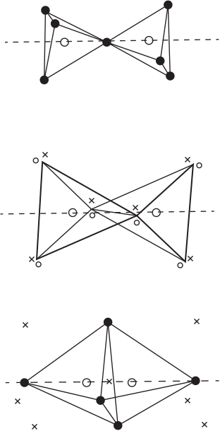
Nodal Regions and Tiles
In 2004, TWS published a paper which described the use of the Voronoi diagram to delineate the same-signed permutation cells (as he then called ‘tiles’) of simple atomic, many-electron wavefunctions.[21] It was found that if a local maximum of the wavefunction (and its permutations) was designated as the Voronoi site(s), the resulting wavefunction tile led to localised electrons (Fig. 8). For the ψ = ∣φ1sφ2p∣ triplet wavefunction of helium, the electrons occupied diametrically opposed regions, like sp-hybrid orbitals. In this case, the hybridisation is a result of antisymmetry. The ψ = ∣φ1sφ2s∣ triplet wavefunction of helium yielded a core, and a valence electron, one always further from the nucleus than the other. The ψ = ∣φ1sφ2sφ2p∣ quartet wavefunction results in a core, and two sp-hybrid like electrons. And so on, the quintet and sextet wavefunctions reveal the emergence of core-sp2 and core-sp3-like tiles, suggesting a relationship to Linnett’s tetrahedra in the latter case.
TWS was then distracted by lasers and spectroscopy until his move to UNSW allowed a degree of academic freedom to pursue this idea further.
Lüchow and Liu
Lüchow and Petz applied the Voronoi diagram to molecules in 2011, showing that, by using a wavefunction maximum as the reference site, as done by TWS in 2004, localised electrons result.[23] The emergent 3N-dimensional wavefunction tile, projected onto the three spatial coordinates of each of the N electrons, in turn, results in the ‘single electron densities’. The lone-pairs of water and the banana-bond description of double bonds emerged as natural motifs. An update to the method, whereby the Voronoi sites were defined by the average position of walkers was reported in 2012 as ‘self-consistent centres of charge’ (SCCC).[24] In order to avoid the factorially expensive search over Voronoi sites necessary to contain walkers, Lüchow and Petz implemented the Hungarian assignment algorithm (also known as the Munkres algorithm). However, this necessitates the Voronoi diagram to not only delineate like-signed tiles but also differently-signed tiles. We feel it is more natural to allow the node to form this boundary.
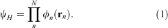
In 2016 we published our first paper on molecules, where the SCCC algorithm was tweaked to allow the nodes to form the boundary between differently signed tiles.[14] A modified Hungarian algorithm (which we call the Canberran) was designed by Philip Kilby of CSIRO’s Data 61 in Canberra, to allow efficient searching of only like-signed tiles. Our method was designated ‘dynamic Voronoi Metropolis sampling’ (DVMS), which describes how the Voronoi diagram updates itself as the walkers sample the electronic wavefunction (squared) according to the Metropolis algorithm.[22] We showed that this algorithm produced structures where the Voronoi site corresponded closely to Linnett’s DQT (Fig. 9a). Many standard molecules such as water, formaldehyde, dinitrogen, and difluorine were found to have DVMS structures in accord with the VSEPR and Linnett models (Fig. 9b). A triumph of sorts was the demonstration that correlated wavefunctions could be illustated in a simple and intuitive manner. C2, after the primary doubly-excited determinant was included, was found to demonstrate an asymmetric triple-bond, and the singlet-coupled non-bonding electrons (which Shaik identifies as the fourth bond, Fig. 9c).

|
Reactions
Since any wavefunction may be analysed in terms of tiles, we sought to apply the DVMS algorithm to chemical reaction paths. The smooth variation of the Voronoi diagram along the reaction path corresponds closely to the ‘curly arrow’ notation of organic chemists.[26] We found that SN2 and nucleophilic carbonyl addition proceeded as per chemistry textbooks. In the attack of hydroxide on formaldehyde, one of the double-bonding sites ‘peels off’ to smoothly morph into a non-bonding site on the carbonyl oxygen (Fig. 10). Our most intriguing finding was that the Diels-Alder reaction of ethylene and cis-butadiene proceeds with anti-correlated up- and down-spins.
|
Excited States
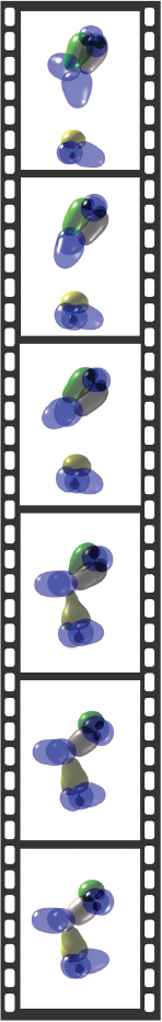
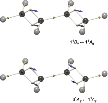
Excited-state wavefunctions also exhibit antisymmetry but will have more nodes and/or different nodes to the ground state. In the spirit of semiclassical theories of spectroscopy, we calculated the DVMS stuctures of ground state molecules and then investigated the motions of the average electron positions as a function of the phase of a superposition of the ground and excited states.[27] The ‘quantum beats’ manifest as the electrons vibrating about their equilibrium positions, as postulated by Lewis![2] In trans-butadiene, the two double bonds were found to combine as in- and out-of-phase vibrations, corresponding to excitation to the 11B1u and 31Ag states respectively (Fig. 11).
|
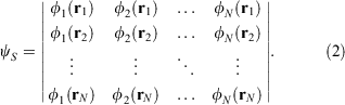
Bent Bonds
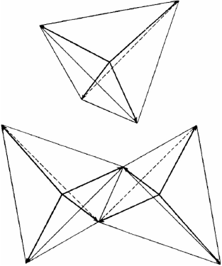
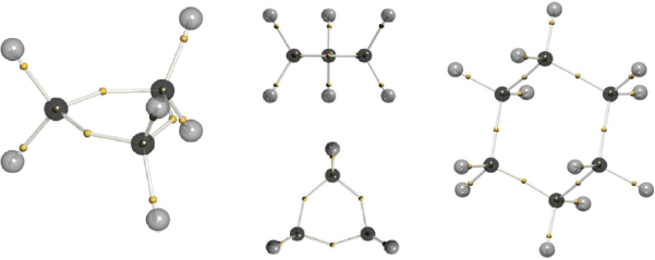
The Voronoi sites generated by DVMS represent average electron positions within the tile, as defined by those average positions. As such, they are a self-consistent solution, but not always a unique solution. Nevertheless, for simple closed-shell molecules the solution is unique, and reproduces motifs such as core electrons, single bonds, double bonds (represented as ‘banana bonds’), and lone-pairs. But, there is more. In cyclopropane, the strain on the single-bonds can be visualised, as seen in Fig. 12. Unlike in unstrained systems, the C-e-C angle in cyclopropane is calculated to be 143°, and far from being 60°, the e-C-e angle is 97°, not too far off the tetrahedral angle. The DVMS structure is compared to that of cyclohexane in Fig. 12.
|
Configuration Interaction: BeOBe
Boldyrev and Simons demonstrated that a multiconfigurational wavefunction is required to correctly describe the BeOBe molecule.[28] We investigated the nature of this using DVMS, by implementing the algorithm with single and two-determinant wavefunctions.
The equilibrated state of BeOBe obtained from DVMS applied to a single-determinant wavefunction is given in Fig. 13. The molecule is a linear structure with oxygen at the centre, possessing an octet of electrons in a cubical arrangement, as Lewis would have drawn. The single-configurational DVMS, on account of a lack of electron correlation, can ‘accidentally’ result in both non-bonding electrons being on the same atom. Such an asymmetric structure is unexpected.
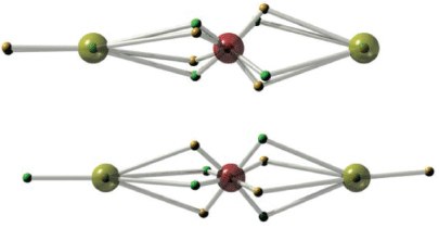
|
The two-configurational DVMS calculation results in the two non-bonding electrons occupying alternative atoms. Where the wavefunction is calculated using MO theory, this sort of correlation results from a doubly-excited determinant whereby the two electrons are promoted from a σg orbital to a σu orbital. The upshot is that, because the coefficient of this double excitation is negative, the probability of occupancy of the same atom is diminished while occupancy of alternate atoms is enhanced. The same type of excitation is at work in C2, and as we shall show in a future paper, allyl cation and ozone.
Conclusions
DVMS has been developed to define and explore the electronic wavefunction tile. The Voronoi sites reproduce the DQT structures of Linnett, and satisfy chemical intuition on many levels. Reactions can be followed by DVMS, which reproduces the ‘curly arrow’ notation of organic chemists. Bright excited states are found to correspond to vibrating structures, as proposed by Lewis in 1916. DVMS can be used to explore multiconfigurational wavefunctions in a way that orbital treatments cannot, and is thus a general way to investigate electronic structure.
Data Availability
The data that support the findings of this study are available from the corresponding author upon reasonable request.
Conflicts of Interest
The authors declare no conflicts of interest.
Acknowledgements
This work was supported by the Australian Research Council (Centre of Excellence in Exciton Science CE170100026).
References
[1] G. N. Lewis, Valence and the Structure of Atoms and Molecules 1923 (Chemical Catalog Company, Incorporated: New York, NY).[2] G. N. Lewis, J. Am. Chem. Soc. 1916, 38, 762.
| Crossref | GoogleScholarGoogle Scholar |
[3] I. Langmuir, J. Am. Chem. Soc. 1919, 41, 868.
| Crossref | GoogleScholarGoogle Scholar |
[4] L. De Broglie, Ann. Phys. 1925, 10, 22.
| Crossref | GoogleScholarGoogle Scholar |
[5] E. Schrödinger, Phys. Rev. 1926, 28, 1049 and references therein.
| Crossref | GoogleScholarGoogle Scholar |
[6] W. Heitler, F. London, Z. Phys. 1927, 44, 455.
[7] J. E. Lennard-Jones, Trans. Faraday Soc. 1929, 25, 668.
| Crossref | GoogleScholarGoogle Scholar |
[8] F. Hund, Z. Phys. 1928, 51, 759.
| Crossref | GoogleScholarGoogle Scholar |
[9] R. S. Mulliken, Phys. Rev. 1928, 32, 186.
| Crossref | GoogleScholarGoogle Scholar |
[10] E. Hückel, Z. Phys. 1931, 70, 204.
[11] L. C. Pauling, Proc. R. Soc. Lond. A Math. Phys. Sci. 1977, 356, 433.
| Crossref | GoogleScholarGoogle Scholar |
[12] L. Pauling, J. Am. Chem. Soc. 1931, 53, 1367.
| Crossref | GoogleScholarGoogle Scholar |
[13] J. W. Linnett, The Electronic Structure of Molecules: A New Approach 1964 (Methuen & Co., Ltd: London).
[14] Y. Liu, T. J. Frankcombe, T. W. Schmidt, Phys. Chem. Chem. Phys. 2016, 18, 13385.
| Crossref | GoogleScholarGoogle Scholar | 27122062PubMed |
[15] J. W. Linnett, J. Am. Chem. Soc. 1961, 83, 2643.
| Crossref | GoogleScholarGoogle Scholar |
[16] H. K. Zimmerman, P. Van Rysselberghe, J. Chem. Phys. 1949, 17, 598.
| Crossref | GoogleScholarGoogle Scholar |
[17] M. J. S. Dewar, H. C. Longuet-Higgins, C. A. Coulson, Proc. R. Soc. Lond. A Math. Phys. Sci. 1952, 214, 482.
| Crossref | GoogleScholarGoogle Scholar |
[18] P. C. Hiberty, S. Shaik, in The Chemical Bond (Eds G. Frenking, S. Shaik) 2014, Ch. 2, pp. 69–90 (John Wiley-VCH Verlag GmbH & Co: Weinheim).
[19] P. C. Hiberty, B. Braïda, Angew. Chem. Int. Ed. 2018, 57, 5994.
| Crossref | GoogleScholarGoogle Scholar |
[20] D. G. Truhlar, P. C. Hiberty, S. Shaik, M. S. Gordon, D. Danovich, Angew. Chem. Int. Ed. 2019, 58, 12332.
| Crossref | GoogleScholarGoogle Scholar |
[21] T. W. Schmidt, J. Mol. Struct. 2004, 672, 191.
| Crossref | GoogleScholarGoogle Scholar |
[22] N. Metropolis, A. W. Rosenbluth, M. N. Rosenbluth, A. H. Teller, E. Teller, J. Chem. Phys. 1953, 21, 1087.
| Crossref | GoogleScholarGoogle Scholar |
[23] A. Lüchow, R. Petz, J. Comput. Chem. 2011, 32, 2619.
| Crossref | GoogleScholarGoogle Scholar | 21638293PubMed |
[24] See Ch. 6, pp. 65–75 in: A. Lüchow, R. Petz, Advances in Quantum Monte Carlo, ACS Symposium Series Vol. 1094, 2012 (American Chemical Society: Washington D.C.).
[25] S. Shaik, D. Danovich, W. Wu, P. Su, H. S. Rzepa, P. C. Hiberty, Nat. Chem. 2012, 4, 195.
| Crossref | GoogleScholarGoogle Scholar | 22354433PubMed |
[26] Y. Liu, P. Kilby, T. J. Frankcombe, T. W. Schmidt, Nat. Commun. 2018, 9, 1436.
| Crossref | GoogleScholarGoogle Scholar | 29651029PubMed |
[27] Y. Liu, P. Kilby, T. J. Frankcombe, T. W. Schmidt, Chem. Sci. 2019, 10, 6809.
| Crossref | GoogleScholarGoogle Scholar | 31391902PubMed |
[28] A. I. Boldyrev, J. Simons, J. Phys. Chem. 1995, 99, 15041.
| Crossref | GoogleScholarGoogle Scholar |
† For the record, the authors do not regard anything as ‘real’, except that which can be measured. However, there is a solution to the many-body Schrödinger equation and we have set it as our task to interpret this solution in terms of canonical chemical concepts.
‡ In a seminar by Prof. Bob Watts at The University of Sydney in the case of TWS; by Dr Harry Schranz in the case of TJF.