

Projecting wildfire emissions over the south-eastern United States to mid-century
Uma Shankar A D E , Jeffrey P. Prestemon B , Donald McKenzie C , Kevin Talgo A , Aijun Xiu A , Mohammad Omary A , Bok Haeng Baek A , Dongmei Yang A and William Vizuete DA Center for Environmental Modeling for Policy Development, University of North Carolina Institute for the Environment, Campus Box 1105, Suite 490, Europa Center, 100 Europa Drive, Chapel Hill, NC 27517, USA.
B USDA Forest Service, Southern Research Station, PO Box 12254, Research Triangle Park, NC 27709, USA.
C Pacific Wildland Fire Sciences Lab, USDA Forest Service, 400 N. 34th Street, Suite 201, Seattle, WA 98103, USA.
D Department of Environmental Sciences and Engineering, University of North Carolina at Chapel Hill, Campus Box 7431, Chapel Hill, NC 27599, USA.
E Corresponding author. Email: shankaruma00@gmail.com
International Journal of Wildland Fire 27(5) 313-328 https://doi.org/10.1071/WF17116
Submitted: 8 August 2017 Accepted: 18 March 2018 Published: 8 May 2018
Journal Compilation © IAWF 2018 Open Access CC BY-NC-ND
Abstract
Wildfires can impair human health because of the toxicity of emitted pollutants, and threaten communities, structures and the integrity of ecosystems sensitive to disturbance. Climate and socioeconomic factors (e.g. population and income growth) are known regional drivers of wildfires. Reflecting changes in these factors in wildfire emissions estimates is thus a critical need in air quality and health risk assessments in the south-eastern United States. We developed such a methodology leveraging published statistical models of annual area burned (AAB) over the US Southeast for 2011–2060, based on county-level socioeconomic and climate projections, to estimate daily wildfire emissions in selected historical and future years. Projected AABs were 7 to 150% lower on average than the historical mean AABs for 1992–2010; projected wildfire fine-particulate emissions were 13 to 62% lower than those based on historical AABs, with a temporal variability driven by the climate system. The greatest differences were in areas of large wildfire impacts from socioeconomic factors, suggesting that historically based (static) wildfire inventories cannot properly represent future air quality responses to changes in these factors. The results also underscore the need to correct biases in the dynamical downscaling of wildfire climate drivers to project the health risks of wildfire emissions more reliably.
Additional keywords: climate and socioeconomic change, emissions projections, wildfires.
Introduction
Wildfires have serious consequences for human health because of the dramatic increase in the concentrations of pollutants of known toxicity emitted in wildfire smoke. There have been several studies (Wegesser et al. 2009; Rappold et al. 2011; Fann et al. 2013) on the adverse health impacts of wildfire-emitted particulate matter (PM) and ozone. Wegesser et al. (2009) found the inherent toxicity of PM from wildfires to be greater than equal doses of PM in ambient air. These researchers have also attributed the toxicity of PM collected from Alaska wildfire sites in their study, in part, to reactive metals as a major source of carbon-centred free radicals, following the findings of Leonard et al. (2000, 2007). Toxic polychlorinated dibenzodioxins and dibenzofurans, and aromatic compounds are also emitted from forest and grassland fires (Gullett et al. 2008). In addition to their adverse health impacts, wildfires can cause extensive damage to human communities and structures and threaten the integrity of some ecosystems that are sensitive to disturbance. For example, in 2016, nearly US$2b of federal funds were spent suppressing wildfires that totalled more than 2.2 × 10⁶ ha (5.5 × 10⁶ acres) on lands managed by the USDA Forest Service and the Department of the Interior (National Interagency Fire Center 2017a). Of these, the overall South-wide costs in 2016 of wildfire suppression of more than 494 000 ha (1.22 × 10⁶ acres) burned were reported at $121m (National Fire and Aviation Management 2017). Wildfires in Smoky Mountain National Park, TN, alone caused up to $2b in damages by some estimates (National Park Service 2017) in late November that year. These are not the only costs of wildfires, however. A large part of the economic impact of wildfires is because of the human health impacts of smoke exposure. Fann et al. (2018) estimate the present combined healthcare costs of mortality and morbidity due to exposure to wildfire-attributable PM less than 2.5 μm in aerodynamic diameter (termed PM2.5) to be $63b (2010 US$) for short-term exposures, and $495b for long-term exposures nationwide. Rappold et al. (2011, 2012, 2014) came to similar conclusions in their study of the health costs of a 45-day peat bog fire in 2008 at the Pocosin Lakes National Wildlife Refuge in rural North Carolina, which was ignited by lightning following a long drought. Rappold et al. (2014) put the costs of emergency department visits during the fire due to excess asthma and congestive heart failure at over $1m, but their estimated costs of general health outcomes, predominantly premature mortality, were $48.4m, far in excess of the medical costs to treat short-term health outcomes.
Climate change has been increasingly implicated in the rise in the frequency and magnitude of large wildfires in the Western US because of the increasing frequency and severity of droughts (Dennison et al. 2014; Stavros et al. 2014; Abatzoglou and Williams 2016). This increasing trend in total area burned has been observed even while the absolute numbers of wildfires has demonstrated a declining trend since the 1960s (National Interagency Fire Center 2017b). Climate change is also expected to lead to longer fire seasons in the south-eastern US by mid-century, as shown in the regional climate model analyses of Liu et al. (2013). However, wildfires in this region are more strongly connected to human factors (Prestemon et al. 2002; Mercer and Prestemon 2005; Syphard et al. 2017). Humans both ignite more fires in this region (Balch et al. 2017) and actively participate in their suppression (Prestemon et al. 2013). Half of the major wildfires in late 2016 in and around Gatlinburg, TN, were attributed to human causes, illustrating the role of humans on wildfire occurrence in this region. Human factors also play a role in wildfire impacts in the form of demographics and income levels of the exposed populations (Gaither et al. 2011; Rappold et al. 2011, 2014). Increased urbanisation and expansion of the wildland–urban interface (WUI) is only expected to increase in the South in the coming decades, increasing the vulnerability of populations to wildfire smoke exposure. In their study of 37 regions across the continental US, Syphard et al. (2017) found wide geographical variability in both the fire–climate relationship, and the role of human presence in fire regimes; their study suggests a geographically complementary role for the two. Thus, region-specific methods of constructing wildfire emissions inventories (EIs) that account for changes in both climate and societal factors are a critical need for better estimating how wildfire emissions and their air-quality impacts will change in the Southeast and managing wildfires and their associated health risks long-term.
Current wildfire EIs, like those used to provide high-resolution inputs (at 12- × 12-km grid spacing or finer) required for air-quality simulations, are typically constructed from the most current data of fire activity and fuel loads selected for their completeness, reliability and accessibility. Empirical data of fire counts for these inventories are provided at the county level in Situation Reports archived and maintained by the USDA Forest Service. They are often augmented by data from satellite remote sensing (RS) of fire pixels detected by the Moderate Resolution Imaging Spectroradiometer (MODIS) instrument, served through the National Oceanic and Atmospheric Administration (NOAA) Hazard Mapping System (Ruminski et al. 2006) and reconciled with ground-based fire reports in the SMARTFIRE emissions processing system (Larkin et al. 2009). The US Environment Protection Agency (EPA) National Emission Inventory (NEI), for example, includes a fire-EI that is updated yearly for its base-year air-quality assessments and forecasting applications using fire activity from the USDA Forest Service Situation Reports, MODIS fire counts from HMS, and fire perimeters from the Monitoring Trends in Burn Severity project (Eidenshink et al. 2007), all of which are processed in SMARTFIRE (Pouliot et al. 2012; Larkin et al. 2014). On-the-ground data that are reported by state and local agencies can also be included once every 3 years, during the NEI release.
Wildfire EIs used in global and regional air-quality modelling characterise the atmospheric loadings attributable to wildfire emissions of pollutants and their precursors under current conditions. Using these inventories in future-year wildfire impact assessments will be wrong from the start (McKenzie et al. 2014) because they do not account for changes in climate, land use, population density or income levels (which may affect emissions exposures – e.g. Rappold et al. 2012). All of these factors are regional drivers in initiating and sustaining wildfires (Mercer and Prestemon 2005) as well as in suppressing them (e.g. Butry et al. 2001). Yet, wildfire inventories used in future-year air quality simulations are based very often on historical wildfire records, without accounting for how changes in climate and other factors could affect future wildfire activity. Future air-quality estimates need to address changes in weather patterns in future years to estimate daily area burned, and methods do exist to do so. For example, McKenzie et al. (2006) projected future daily wildfire activity in the Pacific Northwest region of the US using a stochastic fire-ignition model that estimates daily area burned. These estimates are based on fire weather indices calculated from a mesoscale meteorological-model simulation for the future modelling period. The results of McKenzie et al. (2006) showed that this stochastic method estimated area burned in a historical fire season (2003) over the Pacific Northwest to within 8% of actual burned areas. These estimations, as such, do not include the influences that future changes in population and income could have on wildfire activity. Prestemon et al. (2002, 2016) have shown that such changes are important considerations in the human factors dominating wildfire areas burned in the US Southeast.
The statistical models developed by Prestemon et al. (2016) take into account the combined impacts of climate and socioeconomic factors on wildfire occurrence to estimate AAB at the county level. These multi-stage regression models of historical AABs over the Southeast were used to make multi-decadal projections of future AAB for the region, with fine-scale projections of future climate, socioeconomic factors and land use change as inputs. The statistical models were validated in each stage of their construction against out-of-sample historical observations to eliminate bias. These models of AAB thus provide a framework for the construction of wildfire EIs that allow air quality and exposure assessments to be based on an evolving landscape of natural and human factors influencing fire occurrence, and to project future air quality in the coming decades more realistically in response to potential changes in climate and society.
In this work, we leverage the AAB projection models of Prestemon et al. (2016) that incorporate regional changes in climate, population, income and land use to project daily wildfire emissions in the Southeast, and present the results herein for selected years in the period 2010–2060. We hypothesise and show that wildfire-EIs for the Southeast, if based on historical AABs, will yield significantly different emission levels for criteria pollutants from inventories that do account for these changes. Consequently, we suggest that historical AABs cannot be used to represent the impacts of projected changes in climate and society in the region over the next four decades adequately. Given the uncertainties in the climate change estimates, and the importance of human influences on south-eastern US wildfires, both present and future (Prestemon et al. 2016), realistic wildfire EIs for the Southeast require an integrated method that accounts for expected changes in both climate and society. Model projections of changes in fire activity and fuel loads due to climate change, coupled with projections of human-caused wildfire, could lead to more effective land and wildfire management in a manner that reduces the adverse air-quality impacts of wildfires in future years (McKenzie et al. 2014; Prestemon et al. 2016). The research presented here proposes and tests such a methodology in the south-eastern US. This work is not intended to be an exhaustive study of climate and socioeconomic drivers of wildfires in the Southeast, but rather the description of a feasible, scientifically sound and regionally relevant methodology of constructing wildfire emissions projections that would include the impacts of those drivers, and how they might change in the future.
The emissions-projection methodology developed in this work addresses the stochastic process of wildfires. Although prescribed burns account for more ignitions in the Southeast than do wildfires, they are, by definition, planned fires. They therefore need very different projection methodologies, e.g. incorporating demographic and socioeconomic factors explicitly rather than implicitly through the AABs, as is done here, as well as incorporating different criteria for selecting the burn days. We address these and related issues in the ‘Conclusions’ section.
Methods
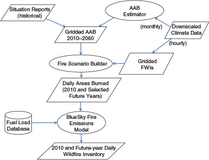
This section describes a dynamic approach to constructing inventories of daily future wildfire emissions by leveraging a readily available statistical model that estimates AAB accounting for changes in climate and society over the five decades from 2010 to 2060. It describes our application of the statistical AAB estimation model of Prestemon et al. (2016) and of the Fire Scenario Builder (FSB) model (McKenzie et al. 2006), which uses these AABs as constraints to estimate daily areas burned based on wildfire ignition probabilities. The daily burned areas are then used in the BlueSky fire emissions model (Larkin et al. 2009) to estimate daily wildfire emissions that are needed as inputs for future air-quality simulations. Fig. 1 shows a schematic of these various models and data flows in constructing a wildfire EI.
|
Annual area burned estimation
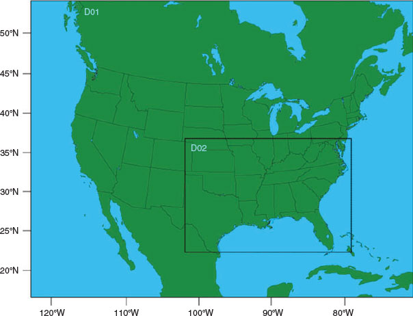
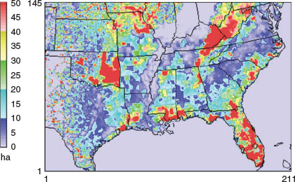
To evaluate the effects of including changes in regional climate and socioeconomics on wildfire activity in the Southeast, our current- and future-year AAB estimates using two different climate downscaling methods are compared against a base case of AABs over the region with no projections of climate or societal influences. A summary of the three AAB estimation methods is provided in Table 1. These are: (1) a base case of historical mean AABs at the county-level calculated with data from 1992 to 2010; (2) a case with AABs that were estimated with the published statistical model of Prestemon et al. (2016) using statistically downscaled meteorological inputs; and (3) a case with AABs estimated with the statistical model of Prestemon et al. (2016) using dynamically downscaled meteorological inputs. The base case, hereafter called ‘historical’, consists of historical mean AABs from the wildfire burned areas compiled from Situation Reports at the county level for 1992–2011 (Short 2014, 2015), because in this first-time application of the FSB to the south-eastern US, we aimed for as similar an implementation to its north-western applications (McKenzie et al. 2006) as feasible. The historical data also provided the AABs used in a static case, i.e. one that does not include changes in climate and socioeconomic factors, to contrast with the other two AAB estimation methods. As empirically accounted for in Prestemon et al. (2016), some counties and years of the 1992–2010 historical period had potentially invalid observations of wildfire areas burned in the Short (2014) database (K. C. Short, pers. comm.). Gap filling of these invalid observations of historical data was done by replacing potentially invalid observations in the Short (2014) database with in-sample predictions of AAB generated with the statistical models of Prestemon et al. (2016). Gap filling accounted for 35.1% of the observations in the region from 1992 to 2010. The county-level historical mean AABs were remapped using a GIS tool on a column–row grid at 12- × 12-km grid spacing over the south-eastern US modelling domain (D02) shown in Fig. 2 for the wildfire inventory development; their sum over this domain is estimated at 450 499 ha (Fig. 3). The historical case is equivalent to a projection of future wildfires in the Southeast that ignores changes in climate and socioeconomic factors, and the 19-year historical mean of AAB (1992–2010) is used as its representative constant value, as shown in the time slices in Fig. 3. For reference, the actual-year AAB for 2010 is also shown in the figure.

|
|
|
To compare against the historical case, two AAB projections were made that do account for changes in climate and socioeconomic factors. Both of them projected the statistical models of Prestemon et al. (2016) onto both 2010 and to future climatology. The first case, hereafter called ‘statistical d-s’, used monthly average values of daily maximum temperature, minimum temperature and potential evapotranspiration (PET – Linacre 1977), and monthly total precipitation as meteorological inputs to the statistical models of Prestemon et al. (2016). In that work, these inputs were taken from historical and projected climate data that were statistically downscaled at 5′ × 5′ resolution (Joyce et al. 2014) using the downscaling relationship of Daly et al. (2002) from each of nine general circulation model (GCM) realisations. The downscaled climate model inputs were remapped using a Lambert Conformal Conic (LCC) map projection over the south-eastern US, to domain D02 (Fig. 2) at 12- × 12-km grid spacing, and aggregated to the required monthly values.
Other key inputs for the statistical model are income and population growth. Projections of these variables were based on three of the greenhouse gas (GHG) emission scenarios (Nakicenovic and Steward 2000) formulated by the Intergovernmental Panel on Climate Change (IPCC) in support of its Third Assessment Report (AR3), which were used in the nine climate realisations (3 GCMs × 3 GHG emission scenarios) reported in Prestemon et al. (2016). The emissions scenarios A1B, representing high economic growth and low population growth, A2, representing moderate economic growth and high population growth, and B2, representing moderate economic growth and low population growth, provided the basis for the income and population growth rates used by Prestemon et al. (2016) for the South-east from the 2010 county-level data to 2060. Historical data needed for projecting population growth at the county level were obtained from the US Census Bureau (2012). Historical annual personal income data by county came from the US Bureau of Economic Analysis (2013a) and were converted to real values (in constant 2005 US$) using the US gross domestic product deflator (US Bureau of Economic Analysis 2013b). Projections of population and income at 5-year increments for each scenario were obtained from the USDA Forest Service (2014), and linearly interpolated for the intervening years. Finally, inputs to the statistical model of changes in land use expected under the future climate scenarios, including those due to changes in the use of forest, cropland, pasture, and urban lands, were estimated at the county level by Wear (2013).
Prestemon et al. (2016) provide justification for using the AR3 scenarios rather than the more currently used Representative Concentration Pathways (RCPs) developed under the IPCC’s Fifth Assessment Report (AR5): unlike the RCPs, the AR3 emission scenarios are directly and mechanistically linked to projections of economic and population growth. These internally consistent socioeconomic projections were also the basis for the county-level projections used by Prestemon et al. (2016) for income and population growth and by Wear (2013) for land uses, which provided the input variables known to be connected to wildfires in the South-east. Updating those projections to be consistent with the RCPs would have required a complete revamp of these region-specific projection data, and was beyond the scope of their work.
The second AAB projection used dynamical, rather than statistical, downscaling of climate model results to provide the meteorological inputs to the AAB estimator, and is hereafter called ‘dynamical d-s’. Meteorological fields for this projection were simulated by a mesoscale meteorological model, the Advanced Research Weather Research and Forecasting (WRF) model, ver. 3.4.1 (Skamarock et al. 2008), forced by dynamically downscaled climate model inputs at its lateral boundaries. The dynamical d-s projection was motivated by the need to examine the effects of using consistent meteorological inputs throughout the inventory development, beginning with the AAB projections, and continuing on to the daily wildfire emissions estimates, as they will also be used later in the hourly air-quality impact assessments. Dynamical, rather than statistical, downscaling has been the practice over the past few decades for generating meteorological inputs for air quality models, because it provides a complete and consistent framework of hourly, 3-D meteorological fields needed to process emissions from all the meteorologically driven sectors (e.g. vegetation, dust, sea spray, fires) and drive the air quality simulations, at the spatiotemporal scales appropriate for tropospheric chemistry and transport of trace pollutants. It is, therefore, important to understand its performance and its limitations to improve the reliability of its projections of wildfire activity and emissions. For comparison with statistical d-s AAB projections, the relevant hourly meteorological fields (minimum and maximum daily temperature, PET and precipitation) from WRF were aggregated to the temporal resolution (monthly) of the predictor variables in the statistical model. Due to its high computational cost, the dynamical downscaling for this comparative study could be done only in selected years over the south-eastern US (domain D02 in Fig. 2), whereas the statistical downscaling could be applied for every year from 2010 to 2060.
The GCM realisation used for the dynamical downscaling and comparison with the statistical d-s results was selected from the publicly available outputs in the North American Regional Climate Change Assessment Program (NARCCAP – Mearns et al. 2009) archive. Provided in this archive were GCM outputs that had been dynamically downscaled with WRF at 50- × 50-km horizontal resolution over the conterminous US (CONUS) domain D01 in Fig. 2. We examined the NARCCAP archive for parent GCM–GHG scenario combinations that matched those used for the statistical downscaling from Joyce et al. (2014), finding only one, the Canadian General Circulation Model, ver. 3 (CGCM3) using the A2 GHG emission scenario, which best fit this criterion. The WRF model results in NARCCAP downscaled from this GCM realisation were then used to provide the lateral boundary conditions (LBCs) for a nested WRF simulation at 12- × 12-km horizontal grid spacing over the Southeast domain. To the extent possible, the same physics options were chosen in WRF ver. 3.4.1 for domain D02 as were used in NARCCAP for domain D01; these options are listed in Table 2. There were differences in the shortwave and longwave radiation schemes and the microphysics parameterisations, because of updates to the WRF model options since the time of the NARCCAP simulations. However, our south-eastern WRF simulations were performed using the nest-down feature in WRF, i.e. using archived boundary inputs extracted from the D01 simulation, rather than as part of a two-way nested multi-domain simulation with D01. The nest-down feature eliminates the possibility of undesired feedbacks from inconsistent schemes between the two domains.

|
Wildfire emissions for the three cases were estimated for a historical year, 2010, for eventual use in air-quality simulations that will be evaluated against ambient observations. As no downscaled data were available for the 2020–2040 period in NARCCAP, the future fire emissions were projected every 5 years beginning with a randomly selected future year – in our case, 2043 – providing inventories for 2043, 2048, 2053 and 2058 (thus the data gap 2010–2043). The random year selection seems reasonable in light of the interannual variability seen in the AAB projections of Prestemon et al. (2016), which nevertheless showed a small but significant increase in projected median AAB over the region, 2056–2060, relative to 2016–2020.
To ensure a robust comparison between the statistical and dynamical d-s methodologies, the AAB projections for the statistical d-s case were then redone in this work using only the downscaled inputs from the CGCM31/A2 climate model realisation. The AABs presented here for the statistical d-s case, therefore, differ somewhat from those published in Prestemon et al. (2016), who reported projected median and uncertainty bands of AABs calculated using all nine climate realisations, even though the underlying statistical models remain the same.
Fire Scenario Builder
The Fire Scenario Builder model (McKenzie et al. 2006) is a stochastic model that estimates daily areas burned at the spatial scales associated with regional climate and air-quality models. The FSB was designed specifically to provide coarse-scale fire areas (as opposed to individual fire perimeters) as inputs to current and future projections of daily fire emissions and smoke dispersion. A detailed schematic of the FSB model is provided in Fig. S1, available as Supplementary material to this paper. Two key assumptions of the FSB are (1) that a fire event in a grid cell will only occur once in a fire season (assuming that fuels cannot return to the landscape within the season), and (2) that a fire season is entirely contained within the calendar year. Using mean AAB associated with some baseline climatology, which is usually historical but not necessarily, the FSB samples a fire-start day randomly from the fire season based on an assigned probability distribution of fire likelihood. This is typically uniform unless informed by particular fire-start data. Here, we use our three estimates of mean AAB – historical, statistical d-s, and dynamical d-s – as baselines for the historical case and the two projections. Although changes in socioeconomic variables are not explicitly input to the FSB, it includes the response of wildfires to changes in socioeconomic factors implicit in the AAB projections. For each model grid cell, the FSB constructs a cumulative distribution of area burned with the AAB for that grid cell as the mean, using a mixed model that is a negative exponential up to the 95th percentile and a truncated Pareto distribution beyond that value. The beginning and end dates of the fire season appropriate for the Bailey ecoregion province (Bailey 1995) allocated to each model grid cell are read from a national database maintained by the USDA Forest Service. Fires are further constrained to burn only if precipitation is less than 5 mm day−1. If it is above that, another fire-start day is sampled.
A fire-weather metric from the historical climatology that can be simulated for the future is chosen as an indicator of potential fire size. The fire-weather metric used in this study is the fire weather index (FWI – Van Wagner and Pickett 1985) from the Canadian Forest Fire Danger Rating System (CFFDRS), and the calculation of this metric is accomplished through its Canadian Forest Fire Weather Index system shown schematically in Fig. S2. FWI is a comprehensive metric that incorporates several measures of heat and dryness, and is used in fire-danger projections in forests within and outside Canada (Liu et al. 2010; Stavros et al. 2014). It is computed from the dynamically downscaled daily meteorology for all selected years. We note that the use of this metric necessitated the use of dynamically downscaled meteorological data in all daily fire emissions estimates, even in the case where the AABs were estimated with statistically downscaled meteorological inputs, because the temporal aggregation (monthly) at which the statistical d-s inputs were available was too coarse to calculate daily FWI. Area burned on the randomly selected fire-start day for each case is calculated as the quantile from the cumulative distribution of AAB that corresponds to the quantile of the FWI from the climatology for that case matching that day’s FWI. Fires as treated by the FSB can burn up to 4047 ha (10 000 acres) per day; larger fires are modelled as multiday fires.
At first glance, the use of our 12- × 12-km spatial resolution may seem too coarse for the FSB, but our selection of this resolution can be understood as follows. The FSB is really simulating annual fire activity as a surrogate for real fire simulation. Actual fires do not burn contiguously for 144 km2 except in extreme events, but the coarse scale (relative to that of typical fires) of the FSB application for air-quality modelling requires a stochastic representation of AAB, the relevant fire metric. Therefore, the area burned in a single year (‘fire’) is simulated by the FSB, constrained probabilistically by the historical mean (or a future-year annual mean). Lumping all possible ‘fires’ in a year into a single ‘event’ would cause drastic information loss at the scale of fire-spread models, but at our coarser scale it is the only tractable way to represent AAB, and actually limits the error propagation that would ensue from attempts to partition burned area into individual ‘fires’ (somewhere within a 12- × 12-km grid cell).
BlueSky fire emissions model
Using the results from the FSB, daily fire emissions were estimated using the BlueSky smoke emissions modelling framework (Larkin et al. 2009) for each of the cases discussed (historical, statistical d-s and dynamical d-s). The BlueSky model accomplishes this by using the gridded daily burned areas in conjunction with fuel load data available in the Fuel Characteristic Classification System (FCCS) database (McKenzie et al. 2007) to estimate daily fire emission rates. BlueSky is a highly modular framework that links state-of-the-science models of meteorology, fuels consumption and emissions, and provides flexibility in the data sources for fire activity and fuel load inputs. Fuels consumption in BlueSky is based on the CONSUME model, ver. 3.0 (Ottmar et al. 2006), the default modelling option, which is an empirical model developed by the USDA Forest Service based on 106 different pre- and post-burn plots covering several vegetation types and fire conditions. Emissions are estimated as daily rates by a fire emissions module for CO, CO2, CH4 and PM2.5. In our application, BlueSky is used at the latitude–longitude location of each fire strictly for estimating total emission magnitudes of the various emitted species. The fire emissions estimated in BlueSky for the ‘fire’ modelled by the FSB are processed in the Sparse Matrix Operator Kernel Emissions (SMOKE) processing system (Houyoux et al. 2000) similarly to other point sources, which are vertically distributed in the air-quality model simulation in a later step (not presented here), using the plume-rise algorithm within that model.
Results
This section presents the comparisons of the historical mean AABs from a retrospective period against those estimated using the climate-downscaling approaches described previously, examining both time slices of AABs aggregated over the south-eastern modelling domain, and their spatial distributions in each modelled year. Similar analyses are then presented of the wildfire emissions of PM2.5 estimated using each set of these AABs.
Comparisons of AAB estimation methods
The purpose of these analyses is to examine the sensitivity of the statistical model estimates of AABs to the downscaling method used to provide their meteorological inputs, because the AABs are used as constraints on the daily burned area estimates needed to calculate wildfire emissions. AABs from the historical mean over a 19-year period, 1992–2010 (inclusive), provide a benchmark to compare against the modelled estimates of AABs using the downscaled climate inputs. These historical mean AABs summed over the domain D02 add up to 450 499 ha, shown as a constant value in Fig. 3 for all years modelled. The spatial pattern of the historical mean AABs is shown in Fig. 4. Prestemon et al. (2016) found that human-caused ignitions, whether accidental or intentional, dominate over lightning-caused ignitions in the peak locations shown in Fig. 4. These occur in the western part of the domain, in Oklahoma, Arkansas and Missouri, along the Gulf coast, in Florida, up the Southeast Coast, and in the Appalachian region. These are regions where there are both an abundance of fuels and ample human populations with access to those fuels.
|
The domain-total AAB estimate in 2048 is much lower than in the other modelled years for the case of statistically downscaled meteorology (Fig. 3). This low estimate can be explained through the interannual variability of the AAB from 2010 to 2060 shown in Fig. S3. As previously noted, the years for our study were selected at an arbitrary interval of 5 years beginning at a randomly chosen year, 2043. In a random year such as 2048, there can be as much as ±50 000 ha difference from the domain-total mean AAB value. The statistical d-s AAB estimates summed over the D02 domain are distributed around, and fall within ±7% of the historical mean AABs, but there are larger negative deviations from the historical mean in 2048 (−20%) and 2058 (−13%). Given the excellent agreement seen in Fig. 3 for this case with the actual AAB value for 2010, the deviation of its AABs projections from the historical mean is a clear consequence of the influences of climate and socioeconomic factors, each with its own variability.
The spatial differences in AAB for the statistical d-s case from the historical case (Fig. 5, left panels) show that in 2010, the positive and negative differences are smaller than those in other years, and largely offset each other. In 2043, there are large negative differences (i.e. historical AABs are much greater than the statistical d-s estimates) in the ecoregion provinces to the north in northern Missouri, offset by a large positive difference in ecoprovinces in Florida and along the Gulf coast. In 2048, the positive differences in these coastal ecoprovinces are not large enough to offset the negative differences in the interior of the domain, and the domain-wide difference is a net negative, consistent with the time-slice plot in Fig. 3. In 2053, the small net-positive difference is due to the positive AAB differences in these coastal ecoregion provinces and much of Texas, outweighing the negative differences in the interior of the domain. Finally, in 2058, the spatial pattern once again shows negative differences dominating over larger areas of the domain, and to a greater extent than in 2010, with little or no contribution from Texas. The net result overall is a negative difference, i.e. lower AAB values in the statistical d-s case than in the historical case.
|
AAB estimates for the dynamical d-s case are significantly lower than in the other two cases in each of the 5 modelled years (Fig. 3). The temporal variability in AAB is also quite different between the two downscaling methods, with the closest agreement in 2048 (a difference of 10 814 ha), and the greatest differences in 2053 and 2010 (182 591 ha and 148 249 ha respectively). Spatial differences in AAB for the dynamical d-s case relative to the historical case (Fig. 5, right panels) show less temporal variability than for the statistical d-s case (Fig. 5, left panels). The greatest negative differences are seen to occur along the Gulf coast and Eastern seaboard, whereas the portion of the domain west and north-west of Missouri is the main contributor to positive differences. These positive differences offset the negative differences across the domain significantly in 2048, consistent with the smallest domain-wide difference in all the years shown in Fig. 3 between the historical and dynamical d-s AAB estimates. Similar spatial offsets of positive and negative differences occur to a lesser degree in 2043 and 2053, although the net result domain-wide in each of these years is still a negative difference (i.e. the historical AABs are greater than dynamical d-s estimates). Unlike the case of the statistical d-s, the Appalachian region in the right panels has a persistent large negative difference, as do parts of the Gulf coast; these are also areas where the historical mean AABs had the largest values (see Fig. 4). As both the downscaling methods used the same parent climate model realisation, these differences in the spatial patterns in Fig. 5 are a result of the differences in the downscaling methods themselves.
The right panels of Fig. 5 show that dynamical downscaling leads to much less wildfire activity in the Southeast, relative to the 19-year historical mean, while statistical downscaling preserves more of the large-scale circulation patterns in the region in the future decade and shows smaller differences from the historical fire activity. Liu et al. (2013) also found such spatial differences in their analyses of future wildfire activity in the dynamically downscaled results with the HRM3 regional climate model (RCM) compared with the HadGCM climate model used in their previous analysis (Liu et al. 2010). Their study over North American regions used the Keetch–Byram Drought Index (KBDI – Keetch and Byram 1968) as the indicator of fire potential and compared the results of the KBDI calculation from RCM results for the different GCM/RCM downscaling combinations in NARCCAP. Although the climate system showed a warming overall in the 2041–2070 period over North America relative to the 1971–2000 period, there were pronounced differences in the locations of peak precipitation and temperature between the HRM3 and the HadGCM. It is worth noting that their 2013 results are at a coarser resolution (50- × 50-km) for the various regions, and used a different GCM/RCM combination to calculate future climate change from the one used in our study (CGCM3/WRFG) over the Southeast. The HRM3 model that they used for their Southeast assessments had the smallest KBDI increase of all the RCMs in NARCCAP in the future decades in the Central Plains and Deep South, the region of our study. By comparison, the WRFG, used to provide boundary inputs for our Southeast WRF simulation, showed more mixed results, with a moderate KBDI increase from warming and drying in the Deep South, but a KBDI decrease in the Central Plains because of increased precipitation in the future. However, our WRF model results for the Southeast are from a nest-down simulation at a 12- × 12-km spatial resolution from the dynamically downscaled WRFG model results in NARCCAP. Any biases, particularly in precipitation, relative to the GCM will be propagated in the boundary inputs extracted from those results and input to our Southeast WRF simulations. Another major difference in our method from the Liu et al. (2013) study is that their study did not consider county-level socioeconomic factors, and used a different indicator of wildfire, the KBDI, from our fire weather metric (FWI) and would be expected to produce different results. We explain this further under ‘Discussion’.
PM2.5 predictions from wildfires
The AABs estimated from the three cases described previously were used to develop wildfire emission inventories suitable for air quality model simulations needed in impact assessments of ambient PM2.5. Fig. 6 shows the variability of PM2.5 emissions from wildfires among the selected years. For this figure, the emission rate of total PM2.5 calculated for each point fire by the BlueSky fire emission model was mapped to the south-eastern US domain (D02) modelling grid using the SMOKE processor (Houyoux et al. 2000), and the gridded daily emissions were vertically integrated and summed over the year in each grid column for each year modelled. Consistent with the AAB estimates from the three cases shown in Fig. 3, the PM2.5 emissions estimates are highest for the historical case, followed by the cases using AABs estimated with statistically and dynamically downscaled meteorology. The historical and statistical d-s total PM2.5 emission trends follow each other closely in 2010 and 2043, whereas the dynamical d-s trends are 50% and 20% lower in these years, and even lower in the later years, except for the maximum in 2048 leading to good agreement with a correspondingly low value mentioned previously in the statistical d-s case. The dynamical d-s estimates of PM2.5 emissions are also the closest of all three cases to the NEI 2010 emission levels from point wildfires, which are shown here for reference. There is slightly less variability in the time slices of wildfire PM2.5 emissions using the historical mean AABs than in the case using statistically downscaled meteorology. As the AAB estimates used to constrain the daily burned areas are constant for the historical case, this emissions variability can be attributed to the mesoscale model calculation of the daily FWI. The tendency of the WRF meteorology is to lower the daily wildfire activity, and, therefore, the emissions, and this is once again evident in these emissions estimates for the historical case, albeit to a far lesser degree than in the dynamical d-s case.
|
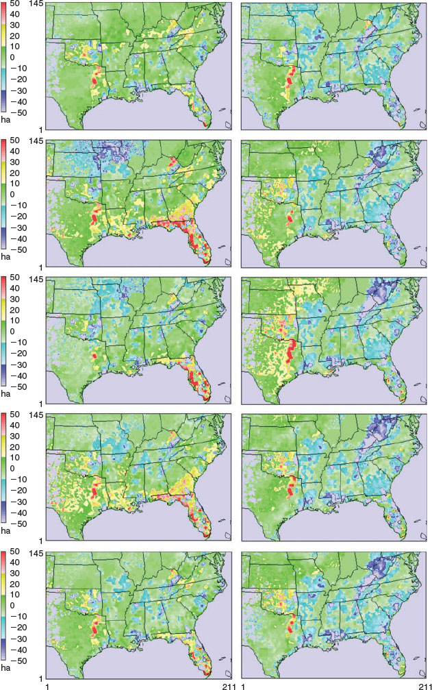
Fig. 7 compares the spatial distributions of PM2.5 emissions using the historical AABs (left panels) against those estimated using AABs from the dynamical d-s case (right panels). For simplicity, the statistical d-s results are not included here, but the comparison of the domain-wide historical v. statistical d-s estimates of wildfire PM2.5 emissions is available as Fig. S4. The PM2.5 emissions for the historical (and statistical) case show greater spatial variability within a given year than for the dynamical d-s case and higher values in the interior Southeast because of the underlying higher wildfire activity in this case. Large differences in the spatial distributions of emissions can be seen between the two cases in any year along the Southeast coastal areas, the Appalachian region, eastern Texas and Oklahoma, and Arkansas and Missouri. Of these, the states to the west (the southern part of ‘Central Plains’ in Liu et al. 2013, 2014) were part of the region where the NARCCAP model combination of CGCM3/WRFG tended to predict more seasonal precipitation in the future years (2041–2070), in both summer and winter, compared with the historical period (1970–2000). The remaining regions, which map approximately to the ‘Deep South’ of Liu et al. (2013, 2014), saw a decrease in precipitation in the summer in the future years, but this decrease was among the lowest for all the model combinations in the NARCCAP suite. These spatial differences in wildfire PM2.5 emissions distributions between the statistical and the dynamical d-s cases, therefore, suggest that precipitation increases have an overriding influence on emissions compared with the temperature increases seen in future years.

|
The spatial distributions of PM2.5 emissions in Fig. 7 in each of the future years are generally consistent with the trends of annual total AABs shown in Fig. 3. The much lower AABs in 2048 for the dynamical d-s case translate into smaller, albeit more numerous, wildfires with lower annual total PM2.5 emissions in Fig. 7. The biggest spatial differences in 2048 relative to the historical case are seen to occur in Appalachia, North and Central Florida, in eastern Texas and Oklahoma, and around the Arkansas–Missouri state boundary.
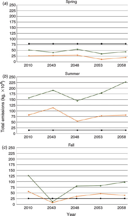
Fig. 8 shows the total seasonal PM2.5 emission estimates for spring, summer and fall (autumn) in each selected year using the historical mean AABs, and those estimated with dynamically downscaled meteorology. Differences in each season between the historical and dynamical d-s cases show the effect of the AAB constraints imposed on the PM2.5 emission rates. Furthermore, the effect of the dynamically downscaled meteorology is seen in the seasonal variability of these emissions. Both the historical AABs and those from the dynamical d-s case yield the lowest emissions of PM2.5 in the spring and the highest in the summer, whereas the NEI estimates for 2010 had the lowest emissions in the summer and higher PM2.5 emissions in both spring and fall. These seasonal plots indicate that the common feature among the historical and dynamical d-s cases, which is the WRF meteorology used to calculate daily FWI, dictates the seasonal variability in wildfire activity in any given year, as well as the variability among the modelled years in each season. In all years, there is also a consistently more pronounced summer high in PM2.5 emissions in the historical than in the dynamical d-s case because of its (constant) higher AAB values. The variability of PM2.5 emissions among the modelled years also somewhat reflects the AAB difference patterns shown in Fig. 5.
|
Discussion
Prestemon et al. (2016) showed that the statistical d-s estimates of AAB reflected the counteracting influences of the climate and socioeconomic variables driving wildfire activity in the Southeast. According to those analyses, the 2056–2060 average annual wildfire areas burned in the Southeast due to human causes would decrease by 6% over the 2016–2020 average in response to changes in socioeconomic influences, but a comparison of the averages over the same periods would show a 34% increase due to lightning-ignited fires, which were minimally influenced by socioeconomic factors. As a majority of areas burned in the southern US are from human causes, the conclusion in that work was that the projected average AAB for 2056–2060 would be higher by ~4% relative to that for 2016–2020 from all causes, with its temporal variability attributable mainly to that of the climate system (see Fig. S3). This variability can also be seen in this work, specifically in the frequency distributions of Fig. 9 of domain-wide totals around the annual mean of the gridded AABs in each year for each of the estimation methods. Given the wide range of the data, values of AAB less than 10 ha are not shown so that the trends around the median values can be seen more clearly. The historical mean AABs used to represent 2010 have a higher median value than either of the other two estimation methods, consistent with the time slices shown in Fig. 3. The statistical d-s AAB distributions have higher maxima than the dynamical d-s distributions in every year, even though their median values are slightly lower than for the dynamical d-s in 2048 and 2058. The higher statistical d-s AABs are also consistent with the domain-total AAB time slices for these two cases (Fig. 3). The effects of competing climate and socioeconomic factors in the AABs for the statistical d-s are also clear in Fig. 3: any biases due to the dynamically downscaled meteorological inputs are not applicable in these AABs. Those biases would, therefore, also have a smaller effect on the PM2.5 emissions in this case (Fig. 6) than in the dynamical d-s case.
|
The WRF model used in the dynamical downscaling yields very different spatial patterns of AAB from the statistical d-s AAB estimates. The differences between the AABs estimated from statistical and dynamical d-s are a consequence of differences between the downscaling methods themselves, as they are both using similar climate model realisations, as well as the same GHG emissions, population, and income growth assumptions, corresponding to IPCC AR3 scenario A2.
The role of the GCM–GHG emissions scenario in the differences seen in the AAB estimates with climate downscaling can be better understood through an examination of their mean changes in temperature and precipitation. Fig. 10 shows the expected changes in precipitation and temperature from 2000 to 2060 from the GCM–GHG emission scenario combinations for the conterminous US, and for the Southeast. In this figure, the CGCM31 scenario A2 shows an increase in precipitation from 2000 to 2060 in both the US and the Southeast, of ~4 and ~6%, respectively, over the ensemble mean for scenario A2. Although this GCM simulation shows a higher-than-mean increase in temperature US-wide, it also shows a slightly smaller-than-mean increase in temperature in the Southeast from 2000 to 2060, compared with the ‘SE A1B&A2’ value. These changes are small for the five-decade period. The change in precipitation is in the correct direction towards explaining the changes seen in the dynamical d-s estimates relative to the historical case, as well as the statistical case, but would likely not be the sole cause of the dramatically lower AAB values for the dynamical d-s case compared with the other two cases.

|
A more likely explanation of the lower AAB values for the dynamical d-s case is 2-fold. One possible reason is the difference between the mesoscale and synoptic-scale predictions, as shown in the regional analyses of wildfire regimes by Liu et al. (2013, 2014). They reported that the dynamical downscaling of climate showed increases in summertime precipitation in the future decades (2041–2070) for the Southeast region (moderate), and South Central region (small) compared with the historical period (1971–2000). This was different from the predictions of the GCM used in their previous studies (Liu et al. 2010). The second likely explanation is the known high bias in precipitation in WRF (Alapaty et al. 2012; Spero et al. 2014), which would also tend to lower the AAB estimates. Dynamical downscaling is also used in the D01 domain to produce the lateral boundary conditions for the Southeast domain, and thus inherits biases in the NARCCAP downscaling with WRF; thus, the influence of the high bias in precipitation in WRF could become magnified, producing consistently lower AABs. This may also account for the differences in our results from those of Liu et al. (2013) for the Southeast, which showed increases in the fire potential indicator (KBDI) by at least one level, and an increase in the length of the fire season in nearly all months. Of note, the Liu et al. (2013) analyses used a single level of dynamical downscaling from the GCM, i.e. only for domain D01, a coarser resolution (50- × 50-km), a different fire potential index, the KBDI, from that of our work (FWI), and did not include county-level socioeconomic changes.
The historical case, which uses historical mean AABs to constrain daily area burned, estimates higher total PM2.5 emissions than the dynamical d-s case for every year and season except in the fall of 2043. These higher values could be partly because of the much higher AABs in some years in the 19-year fire history (e.g. in 2000 and 2006) than in the future projections, as indicated by the lower actual-year AAB for 2010 compared with the 19-year historical mean shown in Fig. 3. Equally important, the historical mean AABs do not include the socioeconomic changes projected in the dynamical d-s case, which were shown to offset the influences of climate warming on the AAB projections in the Southeast (Prestemon et al. 2016). The projected variability in climate and socioeconomic factors from the CGCM3 scenario A2 climate simulation influences the dynamical d-s AAB projections but has no role in the historical AABs. The effects of a wet bias in WRF on the AABs would also be compounded in the PM2.5 emissions by those on the daily FWI inputs to the FSB, leading to lower annual totals and peak values in spatial distributions of PM2.5 emissions in the dynamical d-s case than in the historical case.
The fall wildfire emission levels are lower than summer levels in all years and cases modelled. The possible WRF ver. 3.4.1 overprediction of precipitation and underprediction of temperature appear to have the greatest effect in the fall season fire activity, translating into lower wildfire PM2.5 emissions. Overall, we would expect PM2.5 trends to follow those of the AABs, although the relationship is clearly nonlinear, due to the stochastic nature of the daily disaggregation of the AABs in the FSB as well as the spatiotemporal variability in the downscaled predictions of fire weather. It is clear that the latter will, at a minimum, introduce variability that cannot be inferred from the historical data.
Conclusions and future work
Wildfire area burned, and the resulting emissions of PM2.5 in the Southeast for the period 2010–2060 are seen to be a result of two competing drivers, climate and socioeconomics, each with its own spatiotemporal variability. This may not always lead to uniform increases in wildfire activity and emissions in future climate regimes. The historical mean AABs are higher than those estimated from statistically downscaled meteorology in most of the years modelled, and higher in all years than those estimated with dynamically downscaled meteorology. Historically based estimates of wildfire emissions in the Southeast are consistently higher (by 13–62%) for PM2.5 than those estimated by either of the projection methodologies. The large differences in the temporal variability and spatial patterns of PM2.5 emissions in future years compared with their historical values are attributable in part to the temporal variability of the future climate and socioeconomics underlying the annual area burned projections, and to the dynamically downscaled meteorology used to estimate future daily fire activity. The wildfire emissions estimated from a historical mean of areas burned, even for the most recent 19-year period, do not appear to be representative of how the climate and socioeconomic variables driving wildfire activity and emissions could change in future decades. Our results, therefore, suggest that the use of historical AABs is not sufficient to construct wildfire emission inventories for simulating future-year air quality by mid-century, be they for climate change impact assessments, or for projecting population health risks from wildfire smoke.
This work also shows significant variability among the modelled years in the AABs and the corresponding wildfire PM2.5 emissions as a result of the natural variability of the climate system. Better inferences of temporal trends can be obtained in the dynamical downscaling by ensemble simulations that bracket the extremes in climate and societal change over the 2010–2060 period using representative high- and low-fire frequency years from among several GCM/GHG emission scenarios.
Another finding of this work is that the high bias in precipitation in the WRF model could be the reason for significantly lower wildfire emissions estimates from dynamical downscaling than from statistical downscaling of climate in the AAB estimation model inputs. The effect of the dynamical downscaling of climate on wildfire emissions is important, because this is the most consistent method in current use to calculate meteorological inputs for estimating daily wildfire activity and wildfire emissions, and for driving the air-quality simulations. Thus, we need to understand and correct biases in the dynamical downscaling, particularly as regards precipitation in the Southeast, because of its strong influence on fire weather, and soil and fuel conditions. Less biased downscaling would provide more reliable support of natural resource management and wildfire health risk assessments.
Future contributions from ongoing work will examine the current (2010) and future-year air-quality impacts based on these emissions estimates. Furthermore, fuel loads are expected to respond both to climate and to evolving fire suppression activities in the Southeast. Excessive fuel buildup, for example, has been cited as the cause of the large wildfires in the past two fire seasons in the south-eastern and western US. Fuel load changes were not explicitly included in the modelled wildfire emission estimates, although the land use changes included in the AAB projections do indirectly account for them in the aggregate. Decisions on where and what to burn in managed fires may benefit from tools that incorporate fuel load changes in these dynamic estimates of wildfire emissions.
Conflicts of interest
The authors declare that they have no conflicts of interest.
Acknowledgements
The authors thank Dr Natasha Stavros for her guidance on the use of the Fire Scenario Builder, Dr Linda Joyce for her guidance on the use of the statistically downscaled climate data, and Dr Jared Bowden and Dr Shannon Koplitz for their insightful editorial comments on the manuscript. Dr Michelle Snyder’s assistance with the R package used in the plots is also gratefully acknowledged. We also thank the North American Regional Climate Change Assessment Program (NARCCAP) for providing the data used in this paper. NARCCAP is funded by the US National Science Foundation, the US Department of Energy, the US National Oceanic and Atmospheric Administration, and the US Environmental Protection Agency Office of Research and Development. This research was supported entirely through funding provided by USDA Forest Service to the University of North Carolina at Chapel Hill under joint venture agreement 11-JV-11330143-080.
References
Abatzoglou JT, Williams AP (2016) Impact of anthropogenic climate change on wildfire across western US forests. Proceedings of the National Academy of Sciences 113, 11770–11775.| Impact of anthropogenic climate change on wildfire across western US forests.Crossref | GoogleScholarGoogle Scholar | 1:CAS:528:DC%2BC28Xhs1elur3K&md5=adc1c122ca004fbc9bfa5a07150a254fCAS |
Alapaty K, Herwehe JA, Otte TL, Nolte CG, Bullock OR, Mallard MS, Kain JS, Dudhia J (2012) Introducing subgrid-scale cloud feedbacks to radiation for regional meteorological and climate modeling. Geophysical Research Letters 39, L24809
| Introducing subgrid-scale cloud feedbacks to radiation for regional meteorological and climate modeling.Crossref | GoogleScholarGoogle Scholar |
Bailey RG (1995) Description of the ecoregions of the United States 1995. (2nd edn) USDA Forest Service miscellaneous publication no. 1391, Washington, DC, USA.
Balch JK, Bradley BA, Abatzoglou JT, Nagy RC, Fusco EJ, Mahood AL (2017) Human-started wildfires expand the fire niche across the United States. Proceedings of the National Academy of Sciences of the United States of America 114, 2946–2951.
| Human-started wildfires expand the fire niche across the United States.Crossref | GoogleScholarGoogle Scholar | 1:CAS:528:DC%2BC2sXjsVSlsbo%3D&md5=f30090941422a2b1f6a31439a5d996ddCAS |
Butry DT, Mercer DE, Prestemon JP, Pye JM, Holmes TP (2001) What is the price of catastrophic wildfire? Journal of Forestry 99, 9–17.
Collins WD, Rasch PJ, Boville BA, Hack JJ, McCaa JR, Williamson DL, Kiehl JT, Briegleb B (2004) Description of the NCAR Community Atmosphere Model (CAM 3.0). NCAR Technical Note NCAR/TN–464+STR. (Boulder, CO, USA)
Daly C, Gibson WP, Taylor GH, Johnson GL, Pasteris P (2002) A knowledge-based approach to the statistical mapping of climate. Climate Research 22, 99–113.
| A knowledge-based approach to the statistical mapping of climate.Crossref | GoogleScholarGoogle Scholar |
Dennison PE, Brewer SC, Arnold JD, Moritz MA (2014) Large wildfire trends in the western United States, 1984–2011. Geophysical Research Letters 41, 2928–2933.
| Large wildfire trends in the western United States, 1984–2011.Crossref | GoogleScholarGoogle Scholar |
Eidenshink J, Schwind B, Brewer K, Zhu Z, Quayle B, Howard S (2007) A project for monitoring trends in burn severity. Fire Ecology 3, 3–21.
| A project for monitoring trends in burn severity.Crossref | GoogleScholarGoogle Scholar |
Fann N, Fulcher CM, Baker K (2013) The recent and future health burden of air pollution apportioned across US sectors. Environmental Science & Technology 47, 3580–3589.
| The recent and future health burden of air pollution apportioned across US sectors.Crossref | GoogleScholarGoogle Scholar | 1:CAS:528:DC%2BC3sXktFemsLk%3D&md5=74adfbfca082b2adff67e3cde4305d47CAS |
Fann N, Alman B, Broome RA, Morgan GG, Johnston FH, Pouliot G, Rappold A (2018) The health impacts and economic value of wildland fire episodes in the US: 2008–2012. The Science of the Total Environment 610–611, 802–809.
| The health impacts and economic value of wildland fire episodes in the US: 2008–2012.Crossref | GoogleScholarGoogle Scholar |
Gaither CJ, Poudyal NC, Goodrick S, Bowker JM, Malone S, Gan J (2011) Wildland fire risk and social vulnerability in the Southeastern United States: an exploratory spatial data analysis approach. Forest Policy and Economics 13, 24–36.
| Wildland fire risk and social vulnerability in the Southeastern United States: an exploratory spatial data analysis approach.Crossref | GoogleScholarGoogle Scholar |
Grell GA (1993) Prognostic evaluation of assumptions used by cumulus parameterizations. Monthly Weather Review 121, 764–787.
| Prognostic evaluation of assumptions used by cumulus parameterizations.Crossref | GoogleScholarGoogle Scholar |
Grell GA, Devenyi D (2002) A generalized approach to parameterizing convection combining ensemble and data assimilation techniques. Geophysical Research Letters 29, 1693
| A generalized approach to parameterizing convection combining ensemble and data assimilation techniques.Crossref | GoogleScholarGoogle Scholar |
Gullett B, Touati A, Oudejans L (2008) PCDD/F and aromatic emissions from simulated forest and grassland fires. Atmospheric Environment 42, 7997–8006.
| PCDD/F and aromatic emissions from simulated forest and grassland fires.Crossref | GoogleScholarGoogle Scholar | 1:CAS:528:DC%2BD1cXht1art7zI&md5=682eaf4a195569af673b006cfb73e3a8CAS |
Hong SY, Lim JOJ (2006) The WRF single-moment 6-class microphysics scheme. Journal of the Korean Meteorological Society 42, 129–151.
Hong SY, Dudhia J, Chen SH (2004) A revised approach to ice microphysical processes for the bulk parameterization of clouds and precipitation. Monthly Weather Review 132, 103–120.
| A revised approach to ice microphysical processes for the bulk parameterization of clouds and precipitation.Crossref | GoogleScholarGoogle Scholar |
Hong SY, Noh Y, Dudhia J (2006) A new vertical diffusion package with an explicit treatment of entrainment processes. Monthly Weather Review 134, 2318–2341.
| A new vertical diffusion package with an explicit treatment of entrainment processes.Crossref | GoogleScholarGoogle Scholar |
Houyoux MR, Vukovich JM, Coats CJC, Wheeler NJM, Kasibhatla PS (2000) Emission inventory development and processing for the Seasonal Model for Regional Air Quality (SMRAQ) project. Journal of Geophysical Research 105, 9079–9090.
| Emission inventory development and processing for the Seasonal Model for Regional Air Quality (SMRAQ) project.Crossref | GoogleScholarGoogle Scholar | 1:CAS:528:DC%2BD3cXjtFSgtrY%3D&md5=82948917dd61de11792f2ed26367c0b4CAS |
Iacono MJ, Delamere JS, Mlawer EJ, Shephard MW, Clough SA, Collins WD (2008) Radiative forcing by long–lived greenhouse gases: calculations with the AER radiative transfer models. Journal of Geophysical Research 113, D13103
| Radiative forcing by long–lived greenhouse gases: calculations with the AER radiative transfer models.Crossref | GoogleScholarGoogle Scholar |
Joyce LA, Price DT, Coulson DP, McKenney DW, Siltanen RM, Papadopol P, Lawrence K (2014) Projecting climate change in the United States: a technical document supporting the Forest Service RPA 2010 Assessment. USDA Forest Service, Rocky Mountain Research Station, General Technical Report RMRS-GTR-320. (Fort Collins, CO, USA)
Keetch JJ, Byram GM (1968) A drought index for forest fire control. USDA Forest Service, Southeastern Forest Experiment Station, Research Paper SE-38. (Asheville, NC, USA)
Larkin NK, O’Neill SM, Solomon R, Raffuse S, Rorig M, Peterson J, Ferguson SA (2009) The BlueSky smoke modeling framework. International Journal of Wildland Fire 18, 906–920.
| The BlueSky smoke modeling framework.Crossref | GoogleScholarGoogle Scholar |
Larkin NK, Raffuse SM, Strand TM (2014) Wildland fire emissions, carbon and climate: US emissions inventories. Forest Ecology and Management 317, 61–69.
| Wildland fire emissions, carbon and climate: US emissions inventories.Crossref | GoogleScholarGoogle Scholar |
Leonard SS, Wang S, Shi X, Jordan BS, Castranova V, Dubick MA (2000) Wood smoke particles generate free radicals and cause lipid peroxidation, DNA damage, NFκB activation and TNF-α release in macrophages. Toxicology 150, 147–157.
| Wood smoke particles generate free radicals and cause lipid peroxidation, DNA damage, NFκB activation and TNF-α release in macrophages.Crossref | GoogleScholarGoogle Scholar | 1:CAS:528:DC%2BD3cXms1Sku78%3D&md5=bfd657df0848e91b7dd4b53a47a17582CAS |
Leonard SS, Castranova V, Chen BT, Schwegler-Berry D, Hoover M, Piacitelli C, Gaughan DM (2007) Particle size-dependent radical generation from wildland fire smoke. Toxicology 236, 103–113.
| Particle size-dependent radical generation from wildland fire smoke.Crossref | GoogleScholarGoogle Scholar | 1:CAS:528:DC%2BD2sXlvVyitrg%3D&md5=10d7f6dc84c65018de9ed3f9d260a48cCAS |
Linacre ET (1977) A simple formula for estimating evaporation rates in various climates using temperature data alone. Agricultural Meteorology 18, 409–424.
| A simple formula for estimating evaporation rates in various climates using temperature data alone.Crossref | GoogleScholarGoogle Scholar |
Liu Y, Stanturf J, Goodrick S (2010) Trends in global wildfire potential in a changing climate. Forest Ecology and Management 259, 685–697.
| Trends in global wildfire potential in a changing climate.Crossref | GoogleScholarGoogle Scholar |
Liu Y, Goodrick SL, Stanturf J (2013) Future US wildfire potential trends projected using a dynamically downscaled climate change scenario. Forest Ecology and Management 294, 120–135.
| Future US wildfire potential trends projected using a dynamically downscaled climate change scenario.Crossref | GoogleScholarGoogle Scholar |
Liu Y, Prestemon JP, Goodrick S, Holmes TP, Stanturf JA, Vose JM, Sun G (2014) Future wildfire trends, impacts, and mitigation options in the southern United States. In ‘Climate change adaptation and mitigation management options: a guide for natural resource managers in southern forest ecosystems’. (Eds JM Vose, KD Klepzig) pp. 85–125. (CRC Press: New York, NY, USA)
McKenzie D, O’Neill SM, Larkin N, Norheim RA (2006) Integrating models to predict regional haze from wildland fire. Ecological Modelling 199, 278–288.
| Integrating models to predict regional haze from wildland fire.Crossref | GoogleScholarGoogle Scholar |
McKenzie D, Raymond CL, Kellogg LKB, Norheim RA, Andreu AG, Bayard AC, Kopper KE, Elman E (2007) Mapping fuels at multiple scales: landscape application of the fuel characteristic classification system. Canadian Journal of Forest Research 37, 2421–2437.
| Mapping fuels at multiple scales: landscape application of the fuel characteristic classification system.Crossref | GoogleScholarGoogle Scholar |
McKenzie D, Shankar U, Keane RE, Stavros EN, Heilman WE, Fox DG, Riebau AC (2014) Smoke consequences of new wildfire regimes driven by climate change. Earth’s Future 2, 35–59.
| Smoke consequences of new wildfire regimes driven by climate change.Crossref | GoogleScholarGoogle Scholar | 1:CAS:528:DC%2BC2cXht1Sqt7zP&md5=9e660fb25b49b27079a2145326b74023CAS |
Mearns LO, Gutowski WJ, Jones R, Leung L-Y, McGinnis S, Nunes AMB, Qian Y (2009) A regional climate change assessment program for North America. Earth Observation Systems 90, 311–312.
Mercer DE, Prestemon JP (2005) Comparing production function models for wildfire risk analysis in the Wildland-Urban Interface. Forest Policy and Economics 7, 782–795.
| Comparing production function models for wildfire risk analysis in the Wildland-Urban Interface.Crossref | GoogleScholarGoogle Scholar |
Nakicenovic N, Steward R (Eds) (2000) Special report on emissions scenarios: a special report of Working Group III of the Intergovernmental Panel on Climate Change. (Cambridge University Press: Cambridge, UK) Available at http://www.grida.no/climate/ipcc/emission/index.htm [Verified 14 January 2018]
National Fire and Aviation Management (2017) Southern Area Coordination Center firefighting costs (suppression only). Available at https://fam.nwcg.gov/fam-web/ [Verified 14 January 2018]
National Interagency Fire Center (2017a) Federal firefighting costs (suppression only). Available at http://www.nifc.gov/fireInfo/fireInfo_documents/SuppCosts.pdf [Verified 14 January 2018]
National Interagency Fire Center (2017b) Total wildland fires and acres (1960–2016). Available at http://www.nifc.gov/fireInfo/fireInfo_stats_totalFires.html [Verified 14 January 2018]
National Park Service (2017) Chimney Tops 2 fire review report. Available at https://www.wildfirelessons.net/orphans/viewincident?DocumentKey=5bfa19b8-ca1e-4f4a-882f-9dad173ec28c [Verified 4 February 2018]
Niu GY, Yang ZL, Mitchell KE, Chen F, Ek MB, Barlage M, Kumar A, Manning K, Niyogi D, Rosero E, Tewari M, Xia Y (2011) The community Noah land surface model with multiparameterization options (Noah–MP): 1. Model description and evaluation with local–scale measurements. Journal of Geophysical Research 116, D12109
| The community Noah land surface model with multiparameterization options (Noah–MP): 1. Model description and evaluation with local–scale measurements.Crossref | GoogleScholarGoogle Scholar |
Ottmar RD, Prichard SJ, Vihnanek RE, Sandberg DV (2006) Modification and validation of fuel consumption models for shrub and forested lands in the Southwest, Pacific, Northwest, Rockies, Midwest, Southeast, and Alaska. US Bureau of Land Management, Joint Fire Sciences Program, Final Project Report 98-1-0-06. (Boise, ID, USA)
Pouliot G, Pierce T, Van der Gon HD, Schaap M, Moran M, Nopmongcol U (2012) Comparing emission inventories and model-ready emission datasets between Europe and North America for the AQMEII project. Atmospheric Environment 53, 4–14.
| Comparing emission inventories and model-ready emission datasets between Europe and North America for the AQMEII project.Crossref | GoogleScholarGoogle Scholar | 1:CAS:528:DC%2BC38XmsFejsrw%3D&md5=5942da4e504e8be257ca8144319689f4CAS |
Prestemon JP, Pye JM, Butry DT, Holmes TP, Mercer DE (2002) Understanding broad scale wildfire risks in a human-dominated landscape. Forest Science 48, 685–693.
Prestemon JP, Hawbaker TJ, Bowden M, Carpenter J, Scranton S, Brooks MT, Sutphen R, Abt KL (2013) Wildfire ignitions: a review of the science and recommendations for empirical modelling. USDA Forest Service, Southern Research Station, General Technical Report SRS-171. (Asheville, NC, USA)
Prestemon JP, Shankar U, Xiu A, Talgo K, Yang D, Dixon E, McKenzie D, Abt K (2016) Projecting wildfire area burned in the south-eastern United States, 2011–2060. International Journal of Wildland Fire 25, 715–729.
| Projecting wildfire area burned in the south-eastern United States, 2011–2060.Crossref | GoogleScholarGoogle Scholar |
Rappold A, Stone SL, Cascio WE, Neas LM, Kilaru VJ, Carraway MS, Szykman JJ, Ising A, Cleve WE, Meredith JT, Vaughan-Batten H, Deyneka L, Devlin RB (2011) Peat bog wildfire smoke exposure in rural North Carolina is associated with cardiopulmonary emergency department visits assessed through syndromic surveillance. Environmental Health Perspectives 119, 1415–1420.
| Peat bog wildfire smoke exposure in rural North Carolina is associated with cardiopulmonary emergency department visits assessed through syndromic surveillance.Crossref | GoogleScholarGoogle Scholar |
Rappold AG, Cascio WE, Kilaru VJ, Stone SL, Neas LM, Devlin RB, Diaz-Sanchez D (2012) Cardio-respiratory outcomes associated with exposure to wildfire smoke are modified by measures of community health. Environmental Health 11, 71–80.
| Cardio-respiratory outcomes associated with exposure to wildfire smoke are modified by measures of community health.Crossref | GoogleScholarGoogle Scholar |
Rappold AG, Fann NL, Crooks J, Huang J, Cascio WE, Devlin RB, Diaz-Sanchez D (2014) Forecast-based interventions can reduce the health and economic burden of wildfires. Environmental Science & Technology 48, 10571–10579.
| Forecast-based interventions can reduce the health and economic burden of wildfires.Crossref | GoogleScholarGoogle Scholar | 1:CAS:528:DC%2BC2cXhtlKms7nN&md5=1baf6238f3a3a262edcd06ed624d6d94CAS |
Ruminski M, Kondragunta S, Draxler R, Zeng J (2006) Recent changes to the hazard mapping system. In ‘15th International Emission Inventory conference: reinventing inventories, new ideas in New Orleans’, New Orleans, LA, USA. (EPA) Available at https://www3.epa.gov/ttn/chief/conference/ei15/session10/ruminski_pres.pdf [Verified 14 January 2018]
Short KC (2014) A spatial database of wildfires in the United States, 1992–2011. Earth System Science Data 6, 1–27.
| A spatial database of wildfires in the United States, 1992–2011.Crossref | GoogleScholarGoogle Scholar |
Short KC (2015) Sources and implications of bias and uncertainty in a century of US wildfire activity data. International Journal of Wildland Fire 24, 883–891.
Skamarock W, Klemp JB, Dudhia J, Gill DO, Barker DM, Duda MG, Huang X-Y, Wang W, Powers JG (2008) ‘A description of the advanced research WRF. ver. 3. NCAR/TN-475+STR.’ (National Center for Atmospheric Research: Boulder, CO, USA)
Spero TL, Otte MJ, Bowden JH, Nolte CG (2014) Improving the representation of clouds, radiation, and precipitation using spectral nudging in the weather research and forecasting model. Journal of Geophysical Research: Atmospheres 119, 11682–11694.
| Improving the representation of clouds, radiation, and precipitation using spectral nudging in the weather research and forecasting model.Crossref | GoogleScholarGoogle Scholar |
Stavros EN, Abatzoglou J, Larkin NK, McKenzie D, Steel EA (2014) Climate and very large wildland fires in the contiguous western USA. International Journal of Wildland Fire 23, 899–914.
| Climate and very large wildland fires in the contiguous western USA.Crossref | GoogleScholarGoogle Scholar |
Syphard AD, Keeley JE, Pfaff AH, Ferschweiler K (2017) Human presence diminishes the importance of climate in driving fire activity across the United States. Proceedings of the National Academy of Sciences 114, 13750–13755.
| Human presence diminishes the importance of climate in driving fire activity across the United States.Crossref | GoogleScholarGoogle Scholar | 1:CAS:528:DC%2BC2sXhvFGns7zL&md5=6c49c88a9cbf9c18e156c0d8d88cdde6CAS |
US Bureau of Economic Analysis (2013a) Interactive data. Available at http://www.bea.gov/itable/ [Verified 16 January 2018]
US Bureau of Economic Analysis (2013b) Current-dollar and ‘real’ GDP. Available at http://www.bea.gov/national/index.htm [Verified 16 January 2018]
US Census Bureau (2012) Population estimates. Available at https://www.census.gov/programs-surveys/popest/data/data-sets.All.html [Verified 16 January 2018]
USDA Forest Service (2014) 2010 RPA Assessment population and income data (xlsx). Available at http://www.fs.fed.us/research/rpa/assessment/ [Verified 16 January 2018]
Van Wagner CE, Pickett TL (1985) Equations and FORTRAN program for the Canadian Forest Fire Weather Index System. Canadian Forest Service, Forestry Technical Report 33. (Ottawa, ON, Canada)
Wear DN (2013) Forecasts of land uses. In ‘The Southern Forest Futures Project: Technical Report.’ (Eds DN Wear, JG Greis) USDA Forest Service, Southern Research Station, General Technical Report SRS-GTR-178, pp. 45–71. (Asheville, NC, USA)
Wegesser TC, Pinkerton KE, Last JA (2009) California wildfires of 2008: Coarse and fine particulate matter toxicity Environmental Health Perspectives 117, 893–897.
| California wildfires of 2008: Coarse and fine particulate matter toxicityCrossref | GoogleScholarGoogle Scholar |
Yang ZL, Niu GY, Mitchell KE, Chen F, Ek MB, Barlage M, Longuevergne L, Manning K, Niyogi D, Tewari M, Xia Y (2011) The community Noah land surface model with multiparameterization options (Noah–MP): 2. Evaluation over global river basins. Journal of Geophysical Research 116, D12110
| The community Noah land surface model with multiparameterization options (Noah–MP): 2. Evaluation over global river basins.Crossref | GoogleScholarGoogle Scholar |