
Factors affecting the detection probability of a critically endangered flying-fox: consequences for monitoring and conservation
A. Dorrestein A B * , H. P. R. Rust C D , N. A. Macgregor E F , B. Tiernan G , A. Jankowski G , J. C. Z. Woinarski H , D. J. James I , S. Flakus G , M. Schulz J , S. Pahor G K , A. Mann L , B. Desmond E and J. A. Welbergen A
A
B
C
D
E
F
G
H
I
J
K
L
Abstract
Monitoring is crucial for understanding population trends of threatened species and for assessing the effectiveness of conservation efforts. However, population monitoring is subject to detection probabilities that can vary across factors such as time, type of vegetation cover, weather conditions and observer.
In this study, we investigated the impact of environmental factors (e.g. wind and rain), spatiotemporal factors (e.g. time of night and geographical location) and observer variability, on the detection probability of Pteropus natalis (Christmas Island flying-fox), a critically endangered species that has been monitored across its single (135 km2) island range since 2006, by using active aural and visual detection of foraging individuals.
Surveys were conducted at four visits to 133 sites across Christmas Island, representing the environmental variation of the island, over a 2-month survey period. The survey was conducted in 9 years between 2006 and 2022.
Variable importance analysis showed that distance from the coast, year, and time of night were key predictors of P. natalis detection probability. Detection probability was higher on calmer nights, suggesting higher flying-fox activity or better sound transmission. Detection probability was also higher near roosts earlier and later in the night, indicating that P. natalis gradually moves away from and returns to roosts over the night. Detection probabilities varied between 2012 and 2022 across vegetation types, potentially reflecting changes in diet or phenology. Experienced observers were more likely to detect P. natalis, likely due to familiarity with their vocalisations or visual cues. Analyses excluding environmental and spatiotemporal factors suggested a slight increase in detections since 2012; however, once these factors were included, a significant decrease in detection probability between 2019 and 2022 emerged.
Our findings highlighted how environmental and spatiotemporal factors can affect detection probability and, consequently, survey results of a mobile, threatened small-island endemic.
This study demonstrated the importance of considering environmental and spatiotemporal factors when designing a monitoring program and, in subsequent analysis, to maximise the accuracy and precision of estimates derived from monitoring programs.
Keywords: bats, conservation management, detection probability, flying-foxes, island fauna, observer bias, observer variability, population monitoring, Pteropus.
Introduction
Monitoring populations of any species plays a critical role in decision-making aimed at promoting biodiversity conservation (Marsh and Trenham 2008). It provides valuable information on population status and trends, and on the effectiveness of conservation management (Reddiex et al. 2006; Goldsmith 2012; Westcott et al. 2012; Woinarski 2018). However, obtaining reliable estimates of population size in the wild is inherently difficult (Thompson et al. 1998), and survey methods are subject to various challenges, including accessibility (Wagner 1981; Reddy and Dávalos 2003), animal detection rates (Otto and Pollock 1990), variation in trends across species’ ranges, and between-observer variability (Erwin 1982). Understanding how these factors affect detection patterns is vital to correctly interpret survey data (Hayes 1997), so that they can be confidently used for conservation management.
Monitoring Pteropus (flying-fox) population trends has proven to be especially challenging (Westcott and McKeown 2004; Westcott et al. 2012; McCarthy et al. 2022). Traditional monitoring methods, such as emergence counts or static (‘ground’) counts at colonial roosts (Westcott and McKeown 2004; Forsyth et al. 2006; Oedin et al. 2019), are inadequate for many insular Pteropus species because of their solitary or small group roosting behaviour [e.g. P. tonganus, P. samoensis and P. mariannus (Utzurrijm et al. 2003); P. dasymallus (Vincenot et al. 2017)], and fluctuations in colony size that do not reflect actual population changes (Dorrestein 2023). Surveys of foraging individuals have been proposed as an alternative but may result in overestimations owing to repeated counting of highly mobile individuals (Vincenot et al. 2017). All these challenges may affect detection and can thus affect the reliability of population size estimates of highly mobile mammals such as flying-foxes.
Pteropus natalis (Christmas Island flying-fox) is a medium-sized flying-fox (Todd et al. 2018) endemic to Christmas Island. On this small (135 km2) island in the eastern tropical Indian Ocean, the species fulfills essential pollination and dispersal services and is considered a keystone species (Director of National Parks 2014). However, the species has experienced dramatic population declines since settlement in the early 1900s (James et al. 2007; Woinarski et al. 2014), and is now recognised as critically endangered under the Australian Environment Protection and Biodiversity Conservation Act 1999 (Australian Government 1999). Continued monitoring of the population is vital to inform its management and conservation.
Monitoring the P. natalis population is challenging because of the species’ partially diurnal behaviour (Tidemann 1985; James et al. 2007; Dorrestein 2023) and because a considerable proportion of individuals roosts alone or in small groups, away from the large colonies present at the five permanent roost sites (Tidemann 1985; James et al. 2007; Dorrestein 2023). The primary monitoring approach, applied since 2006, involves nocturnal surveys at numerous fixed locations across Christmas Island, providing relative population trends (Woinarski et al. 2014). However, this method could be subject to potential errors caused by variability in detection of flying-foxes among observers and because of environmental conditions (Erwin 1982; Otto and Pollock 1990). As this monitoring program generates the primary data used to inform management of the species, understanding the factors affecting P. natalis detection probability by using this method is crucial.
In this study, we investigate temporal trends and the effects of various factors on the detection of P. natalis, to improve the reliability of population trend estimates, and so enhance conservation management of this critically endangered species. Specifically, we examine the effects of spatiotemporal factors (such as geographical location, time of night and day of the year), environmental factors (such as vegetation, rain and wind) and among-observer variability on the detection probability of P. natalis, and assess the importance of each examined effect. The implications of our findings for current monitoring practices and interpretation of trend data are discussed.
Methods
Study area
Christmas Island (10°25′S, 105°40′E) is a small (135 km2) remote territory of Australia located in the Indian Ocean, approximately 380 km south of Java. Reaching up to 361 m above sea level, the island is composed of a series of limestone terraces, overlaying basalt and volcanic andesite (Tidemann et al. 1994). The island has a tropical climate, with distinct dry (July–October, average rainfall of 68 ± 14 mm/month) and wet seasons (November–June, average rainfall of 239 ± 25 mm/month) (Australian Bureau of Meteorology 2021). Since settlement in 1888, approximately 25% of the island’s native forest has been cleared for residential development and ongoing phosphate mining. However, 75% of the original forest extent remains, with a national park encompassing 63% of the island.
Sampling method
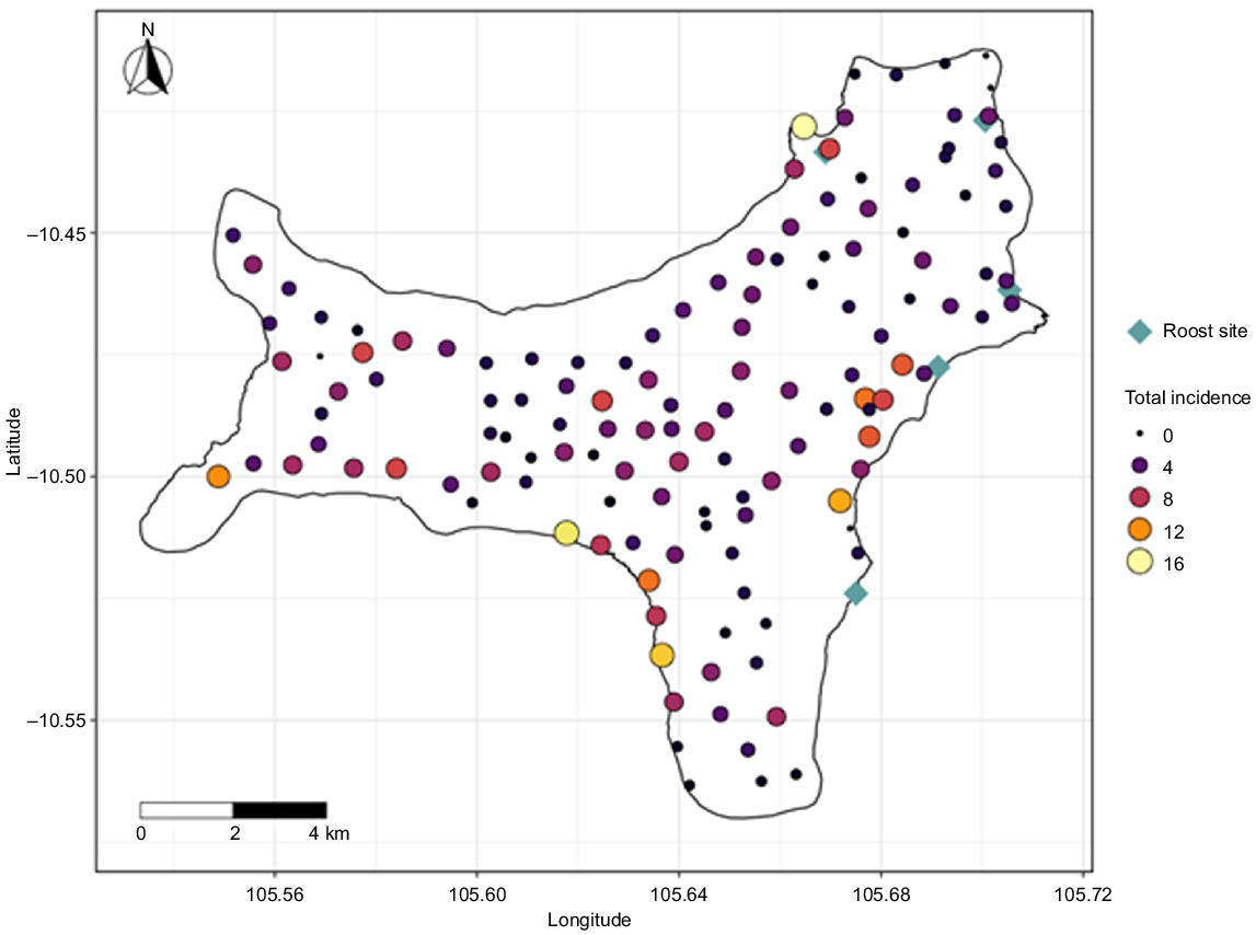
In 2006, a nocturnal monitoring method was established to assess the incidence of foraging P. natalis and to show population trends (Woinarski et al. 2014). Initially, 109 sites across the entirety of the island were chosen, situated adjacent to roads and tracks to ensure accessibility. The sites were more or less evenly spread (0.5–1 km apart) and represented the environmental variation of the island (Woinarski et al. 2014). In the next survey in 2012, two sites were dropped, and 17 sites were added to provide a better coverage of the island, with the resulting 124 sites being sampled in all subsequent surveys. In 2019, following a recommendation to add sites in proximity to current or historic roost sites (Director of National Parks 2016), nine sites were added, bringing the total to 133 sites, which were surveyed in 2019 and 2022 (Fig. 1). In total, surveys have been conducted in 2006, annually between 2012 and 2017, in 2019 and 2022 (Supplementary Table S1).
Sampled sites across the island. Summed detections of Pteropus natalis across all the survey years (2006–2022). Both colour and size of the points represent the incidence. The blue diamonds depict the five major known roost sites.
All sites were sampled four times during each survey period. The observer would approach the site to within 30 m of the predetermined GPS point. The site was approached as silently as possible, and on arrival, sampling would commence as quickly as possible. The time and weather conditions, using the Beaufort scale for wind and presence/absence for rain, were recorded. In 2006, rain was not recorded, and wind was scored as ‘low’, ‘medium’ and ‘high’. For a period of 10 min, the observer would visually inspect the vegetation by using a high lumen headtorch, for example, a Ledlenser H14R.2 headtorch (1000 lumens), for the presence of P. natalis and listen for vocalisations or the distinctive loud wingbeats of P. natalis. The time was noted for each detection, and the distance of the observer to the animal was estimated. Although the aural detection range for flying-foxes has not been formally tested, a study on large forest birds with bodyweights similar to those of P. natalis demonstrated detection ranges of up to 400 m under various environmental conditions (Winiarska et al. 2024). Given the loud vocalisations of P. natalis, we therefore assumed a similar detection range of up to 400 m. For aural detection, no count data were used, owing to the difficulty of estimating group size from vocalisations, wingbeats, and landing sounds, and a P. natalis detection was therefore scored as present. All sampling was conducted between 18:15 hours and 01:15 hours, with the majority of the samples starting before 23:00 hours. Sites were not sampled when wind speeds exceeded 4 on the Beaufort scale [5.5–7.9 m/s], during moderate to heavy rainfall, or when post-rain throughfall hindered aural detections. Sites were never sampled more than once in a night and, where possible, there was at least 1 week between samples at a site.
To aid consistency, surveys were always conducted between the end of May and mid-August. These months were originally selected because they comprise the dry season, lowering the probability of rain impeding the survey. Because these months follow the time when most young have become volant (Todd et al. 2018), this increases the probability that free-flying young are included in the survey.
Statistical analyses
Data analyses for this study were conducted in the R environment (R Core Team 2021) via the RStudio interface (ver. 2024.12.1+563; see https://posit.co/download/rstudio-desktop/; RStudio Team 2020). A significance level (α) of 0.05 was used for all statistical tests. Throughout, we define detection probability as the probability of detecting one or more P. natalis at a site. We refrain from using the term ‘detectability’, because in this study we cannot discern between true and false negatives, because foraging individuals could be silent and masked by foliage and thus go undetected.
Originally for this survey, incidence scores (number of samples with a detection) and mean incidence scores (incidence score/number of sites) were calculated and compared across years (Woinarski et al. 2014; Schulz 2019). We calculated a mean incidence score for the same 107 original sites as used in 2006, the 124 sites as used since 2012, and the 133 sites as used since 2019. A distribution index (DI) was calculated by dividing the number of sites with detections by the total number of detections (Director of National Parks 2016).
To assess the effect of vegetation type on P. natalis detection probability, we used a vegetation and clearing dataset that is freely available online (Walker et al. 2014). The vegetation type data were obtained by extracting the areal extent of nine different vegetation types (closed canopy evergreen forest, coastal fringe vegetation, not vegetated, perennial wetland forest, regrowth, rehabilitation, semi-deciduous forest, semi-deciduous scrub, and weed-dominated vegetation and pioneer regrowth) within a 200-m radius from the GPS point for each site using the sf package (ver. 1.0-20; see https://cloud.r-project.org/web/packages/sf/index.html; Pebesma 2018). The radius of 200 m was chosen as the vast majority of P. natalis detections (88.8%) were within 200 m of the observer. The area per vegetation type was then changed to a percentage for each 200-m sample buffer.
Given that the areal extent of the nine vegetation types for each site add up to the area of a circle with a 200-m radius, these nine variables are necessarily non-independent. To address this, we first performed non-metric multidimensional scaling (NMDS) by using the ‘Bray’ method in the vegan package (ver. 2.6-10; see https://cran.r-project.org/web/packages/vegan/index.html), to visualise the data in a two-dimensional cartesian space defined by the areal extent of vegetation types surrounding all survey locations. The vegetation types were then fitted onto the NMDS. The NMDS yielded a stress value of 0.113, which is considered a reliable fit (Clarke 1993). However, some distortion in the ordination space is possible, meaning that the distances between points may not perfectly represent the true dissimilarities, and interpretations should be cautious, especially for closely spaced or widely separated points. The NMDS should be viewed as indicative rather than exact. Two convergent solutions were found after 20 attempts, and the data underwent centring, PC rotation and half-change scaling. Next, we performed a permutational multivariate ANOVA (PerMANOVA) with 999 permutations to analyse the variance of the distance matrix. This tested whether there was geometric partitioning of variation between sites with and without a flying-fox detection. The scores from the two NMDS axes, NMDS1 and NMDS2, were extracted for further analysis.
To model the detection probability of P. natalis as a function of temporal, spatial, and environmental variables, we used a generalised additive model (GAM) implemented in the mgcv package (ver. 1.9-3; https://cran.r-project.org/web/packages/mgcv/index.html; Wood 2011).
Variables first had to be standardised across survey years. During the 2006 survey, wind was categorised as ‘low’, ‘medium’, or ‘high’. ‘Low’ corresponded to values of between 0 and 1 on the Beaufort scale [0–1.5 m/s], and were thus transformed to a value of 0.5 on the Beaufort scale; similarly, ‘medium’ was transformed to a value of 2.5 on the Beaufort scale [1.6–5.4 m/s], and ‘high’ was transformed to a value of 4.5 on the Beaufort scale [5.5–10.7] (Woinarski et al. 2014). During all other surveys, where wind was recorded as 3–4, or similar, the midpoint value was assigned (e.g. 3.5). The ‘rain’ variable was transformed to ‘presence’ or ‘absence’ of rain. Distance of the sample sites from the coastline and from the nine established roost sites [i.e. those used by multiple GPS-tracked flying-foxes, for multiple nights, in Dorrestein (2023)] was calculated using the osmdata package (ver. 0.2.5; https://cran.r-project.org/web/packages/osmdata/index.html; Padgham et al. 2017). Locations of the established sites were shown in a previous GPS study, where it was also shown that P. natalis was most likely to roost at these sites during the dry season (Dorrestein 2023), which coincides with our study period. Including observer as a factor rendered the model unstable, owing to the large number of people who had conducted the surveys across the years. Therefore, we assigned an experience level ranging from one to four to each observer, based on their experience with the island’s ecosystem, with bats in general, and with P. natalis specifically. We then used the assigned experience level in the model instead of observer.
GAMs were selected for their flexibility in modelling non-linear relationships and their ability to account for complex spatial and temporal patterns. The model had P. natalis detection (yes/no) as the binomial response variable. The initial model included tensor product smooths, which allows for anisotropy, for the interaction between ‘northing’ (continuous) and ‘easting’ (continuous) to capture spatial autocorrelation and location-specific effects. To capture seasonal variations across years, a tensor product interaction was applied to ‘year’ (continuous) and ‘day of the year’ (continuous). Another tensor product interaction modelled the interaction between ‘distance from the roost’ (continuous) and ‘time of night’ (continuous), allowing us to explore how P. natalis movement patterns might change as the night progresses. A further tensor product interaction was used to model a two-dimensional isotropic smooth for ‘NMDS1’ and ‘NMDS2’ (both continuous), combined with a one-dimensional smooth for ‘year’. This term assesses how the association between vegetation type composition and the detection may vary over time, potentially reflecting shifts in resource use or availability across years.
A separate smooth was applied for ‘year’, to specifically assess temporal changes in detection probability, which is a key focus for conservation management. Additionally, a separate smooth was applied to ‘time of night’ to account for potential observer fatigue or changes in P. natalis activity throughout the night. We also applied a smooth to ‘wind’ (continuous) to capture how higher wind speeds may affect P. natalis activity or the observer’s ability to aurally detect P. natalis. A smooth was also applied to ‘distance to the coast’ (continuous), on the basis of previous findings that P. natalis forages closer to the coast during the dry season (Dorrestein 2023). The ordinal factor ‘observer experience’ was converted into a numeric variable to apply a smooth term, preserving its ordinal structure and allowing for flexible, non-linear modelling. We used thin plate splines for multidimensional smooths for their flexibility and ability to handle complex patterns. Cubic regression splines were chosen for univariate smooth terms for their computational efficiency. Rain (binary) was included as a parametric term, owing to its binary nature. A random intercept was fitted for ’site’ (categorical; 133 levels), to account for site-specific variations. Two GAMs were constructed, one including data from 2006 without rain and wind as variables, because these were not recorded in 2006, and another with rain and wind but excluding the 2006 data.
The models were fitted using restricted maximum likelihood (REML) estimation, incorporating a penalisation parameter to shrink non-informative smooth terms automatically to zero. Basis dimensions (k) were initially chosen automatically on the basis of the data. If diagnostic checks indicated issues, adjustments to k were made using the ‘k’-index and associated P-values to ensure the appropriate level of smoothing. We checked for potential concurvity between smooth terms, to ensure model interpretability. We assessed residuals visually and calculated whether the model showed overdispersion. Temporal autocorrelation was checked using the autocorrelation function and the partial autocorrelation function. Spatial autocorrelation was checked using variograms and Moran I test. Model fit was further evaluated by examining residual diagnostic plots. Final model selection was based on the corrected Akaike information criterion (AICc) (Hurvich and Tsai 1989), explained deviance and residual deviance, and guided by REML scores, balancing goodness of fit with model complexity. The model performance in distinguishing between detections and no detections was evaluated using the area under the curve (AUC) of the receiving operating characteristic (ROC) curve. Temporal trends in detection probability were further investigated by extracting slope estimates and their corresponding confidence intervals from the smooth function for the ‘year’ variable. Partial effects including the baseline probability were visualised by extracting the contribution of each smooth term in the model, rather than predicting the overall response, and plotted using the gratia (ver. 0.10.0; see https://gavinsimpson.github.io/gratia/), cowplot ( ver. 3.5.0; see https://wilkelab.org/cowplot/), and ggplot2 (ver. 3.5.1; https://cran.r-project.org/web/packages/ggplot2/index.html; Wickham 2016) packages.
To evaluate the importance of each variable in the GAM, we first employed variable importance plots (VIPs), using the vip package (ver. 0.4.1; https://cran.r-project.org/web/packages/vip/index.html; Greenwell and Boehmke 2020). The importance of each variable was assessed using permutation-based methods, measuring the impact of each variable on model accuracy. The model used for VIP analysis was trained with the same dataset as used for the GAM. We assessed the impact of excluding each variable on model performance by comparing predictions from the most supported model with those from reduced models excluding individual terms. To assess the unique and shared contributions of each predictor to total explained deviance, we performed hierarchical partitioning using the gam.hp package (ver. 0.0-3; https://cran.r-project.org/web/packages/gam.hp/index.html; Lai et al. 2024).
To further investigate how observer experience affected detection probability, we analysed the data from 2022, because we have accurate knowledge on the observers experience level from that year. Observer A had intimate knowledge of P. natalis’ roosting and foraging ecology, having conducted their PhD on the species. Observer B had experience researching microbat calls, but had limited experience with flying-fox vocalisations. To provide insight into the effect of observer experience, we graphed the distances at which P. natalis was detected for the different observers. Observers did not sample the same sites simultaneously. Detection distance was also graphed for Observer C, who conducted the surveys in 2019, to compare Observer A and B to an observer with a lot of flying-fox and surveying experience, but no P. natalis specific experience. We used a two-sample Kolmogorov–Smirnov test to assess whether the distribution of detection distances differed significantly between Observer A and Observer B.
Results
Across all survey years, P. natalis were detected at 97.8% (N = 130) of the 133 sites surveyed across the island. However, within survey years, the number of sites with detections ranged from 31 to 53 (23–40%). The distribution of the detections across all survey years showed that P. natalis individuals were predominantly detected near the coast and near permanent roost sites (Fig. 1; see Supplementary Fig. S1 for detections for each survey year).
Detection trends
The mean incidence score for all 133 sites visited in 2022 was 0.451, which is a decrease from the mean incidence score of 0.586 obtained in 2019. The mean incidence scores for the 124 sites and the original 107 sites were 0.434, and 0.421 respectively (Table 1, Fig. 2).
| Item | Number of sites (samples) | 2006 | 2012 | 2013 | 2014 | 2015 | 2016 | 2017 | 2019 | 2022 | |
|---|---|---|---|---|---|---|---|---|---|---|---|
| Incidence score (number of samples with at least one detection) | 133 (532) | – | – | – | – | – | – | – | 78 | 60 | |
| 124 (496) | – | 58 | 57 | 40 | 65 | 63 | 54 | 68 | 54 | ||
| 107 (428) | 77 | 50 | 48 | 38 | 57 | 48 | 44 | 60 | 45 | ||
| Mean incidence score (incidence score/number of sites) | 133 (532) | – | – | – | – | – | – | – | 0.586 | 0.451 | |
| 124 (496) | – | 0.468 | 0.460 | 0.323 | 0.524 | 0.508 | 0.435 | 0.548 | 0.435 | ||
| 107 (428) | 0.720 | 0.467 | 0.449 | 0.355 | 0.533 | 0.449 | 0.411 | 0.561 | 0.421 | ||
| Distribution (number of sites with detections) | 133 (532) | – | – | – | – | – | – | – | 50 | 41 | |
| 124 (496) | – | 41 | 42 | 32 | 59 | 49 | 40 | 45 | 37 | ||
| 107 (428) | 47 | 35 | 35 | 30 | 53 | 39 | 33 | 41 | 31 | ||
| Distribution index (distribution/number of detections) | 133 (532) | – | – | – | – | – | – | – | 0.64 | 0.68 | |
| 124 (496) | – | 0.71 | 0.74 | 0.80 | 0.91 | 0.78 | 0.74 | 0.66 | 0.69 | ||
| 107 (428) | 0.61 | 0.70 | 0.73 | 0.79 | 0.93 | 0.81 | 0.75 | 0.68 | 0.69 |
Mean incidence scores for the different survey years. Mean incidence score is calculated for 133 sites, 124 sites and 107 sites where applicable. Error bars represent the standard error.
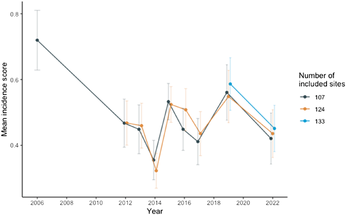
When including only the original 107 sites, the distribution of detections (i.e. the number of sites with detections) in 2006 was higher than in all other years except 2015. The distribution in 2015 was the highest, with detections at 53 sites. The distribution index (DI; number of sites with detections/number of detections) did not change much across the years, averaging 0.72, except for 2015, when the DI was closer to 1 (Table 1).
Vegetation
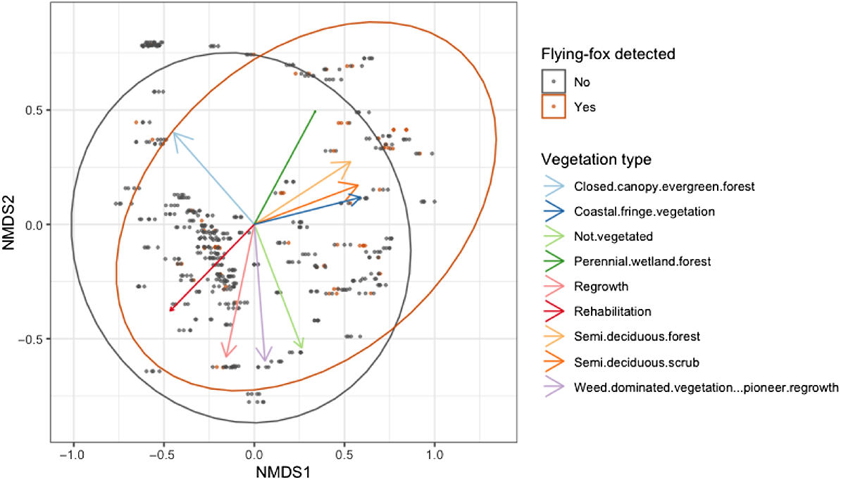
There was a small but significant difference in vegetation composition between samples with P. natalis detection and without P. natalis detection (R2 = 0.006; P = 0.001; Fig. 3). The low R2 indicates that the vegetation composition alone explains a small proportion of the variation in detection patterns. However, although subtle, the difference is significant and thus unlikely to be due to random chance. Sites with higher scores of both NMDS1 and NDMS2 were more likely to have a P. natalis detection. The scores and fitted arrows, a visualisation of the scores, of vegetation types suggest that NDMS1 and NMDS2 are positively associated with a higher areal extent of semi-deciduous scrub, semi-deciduous forest, and coastal fringe vegetation (Fig. 3, Table 2). Perennial wetland also had high scores but had poor fit (R2 = 0.062; Table 2).
Non-metric multidimensional scaling of the areal extent of nine vegetation types in a 200-m radius around 133 sites visited for sampling. Arrows show the fitted vegetation types, the size of the arrowheads represent the relative R2 value. Dark grey points are samples without a flying-fox detection, and dark orange points are samples with a flying-fox detection.
| Vegetation type | NMDS1 | NMDS2 | R2 | P-value | |
|---|---|---|---|---|---|
| Closed canopy evergreen forest | −0.788 | 0.615 | 0.853 | >0.001 | |
| Not vegetated | 0.549 | −0.836 | 0.431 | >0.001 | |
| Regrowth | −0.151 | −0.988 | 0.633 | >0.001 | |
| Weed dominated vegetation and pioneer regrowth | 0.199 | −0.980 | 0.662 | >0.001 | |
| Rehabilitation | −0.741 | −0.672 | 0.181 | >0.001 | |
| Semi-deciduous forest | 0.873 | 0.488 | 0.852 | >0.001 | |
| Semi-deciduous scrub | 0.928 | 0.373 | 0.816 | >0.001 | |
| Perennial wetland forest | 0.525 | 0.851 | 0.062 | >0.001 | |
| Coastal fringe vegetation | 0.938 | 0.346 | 0.498 | >0.001 |
Significant P-values are depicted in bold.
Model performance
During model refinement, we excluded northing and easting from the final GAMs because of high concurvity. Rain was also removed, because this resulted in a lower AICc (Table S2), no change in deviance and an increase of 0.1 in REML score. Further removal of variables did not result in a better fitting model (Table S2). The most supported GAM did not show temporal or spatial autocorrelation (Moran I statistic standard deviate = −2.1482, P = 0.9842), nor overdispersion (0.853). The model AUC was 0.7643, indicating that the model was reasonably effective in predicting detection and non-detection events, on the basis of the environmental and spatiotemporal variables considered. Deviance explained by the model was 12.1%.
The most supported GAM that included data from 2006 but excluded weather variables, also excluded northing and easting because of high concurvity. This model retained all other explanatory variables (Table S2). However, it explained less deviance than did the model including wind. Consequently, our results will focus primarily on the model including weather data, but excluding data from 2006, although we will refer to the model including data from 2006 when discussing the effect of year.
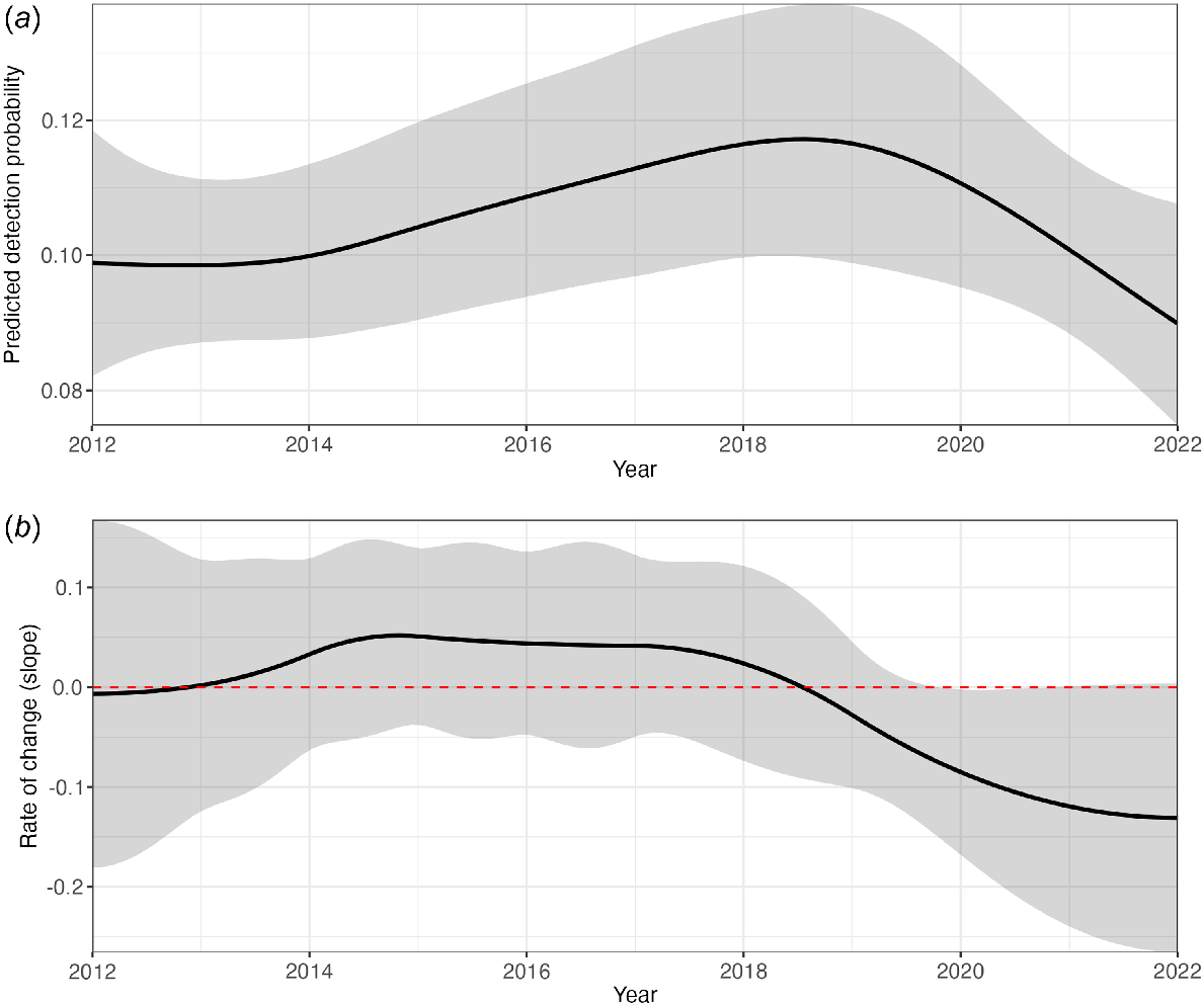
Detection probability changed significantly with year and day of the year (Table 3). While graphing the effects of year on the mean incidence score suggested a slight increase in detections since 2012 (Fig. 2), a different pattern was detected when considering external variables by using GAMs (Fig. 4a). Detection probability increased between 2012 and 2018, after which the probability decreased again (Fig. 4a). However, the slope estimates show that the decrease in detection probability with year is significant (i.e. the confidence interval does not include 0) only briefly, in 2020 (Fig. 4b).
| Item | Model excluding 2006 | Model including 2006 | |||||
|---|---|---|---|---|---|---|---|
| Effective d.f. | χ 2 | P-value | Effective d.f. | χ 2 | P-value | ||
| Year × day of the year | 2.280 | 10.012 | 0.003 | 1.473 | 9.019 | 0.002 | |
| NMDS1 × NMDS2 × year | 1.429 | 4.897 | 0.038 | 4.111 | 36.313 | >0.001 | |
| Distance from the roost × time | 2.141 | 7.806 | 0.018 | 1.903 | 6.543 | 0.025 | |
| Year | 1.543 | 4.445 | 0.042 | 0.716 | 2.555 | 0.062 | |
| Time | 0.698 | 2.888 | 0.076 | 1.450 | 7.537 | 0.012 | |
| Wind | 0.886 | 11.187 | 0.004 | – | – | – | |
| Distance from the coast | 1.857 | 43.624 | 0.006 | 1.562 | 24.895 | 0.022 | |
| Experience class | 0.524 | 1.135 | 0.117 | 0.806 | 4.338 | 0.021 | |
| Site | 74.442 | 193.476 | 0.000 | 74.480 | 189.374 | >0.001 | |
Results of the most supported generalised additive model of Pteropus natalis including data from 2006, which excluded wind data, are shown on the right. Significant values are shown in bold.
(a) Predicted detection probability of Pteropus natalis as a function of year; confidence intervals are depicted in grey. Shown are the predicted probabilities with the intercept added to account for baseline detection probabilities. (b) The rate of change for year. When the confidence intervals (grey) do not include 0 (red dashed line), the rate of change is significant.
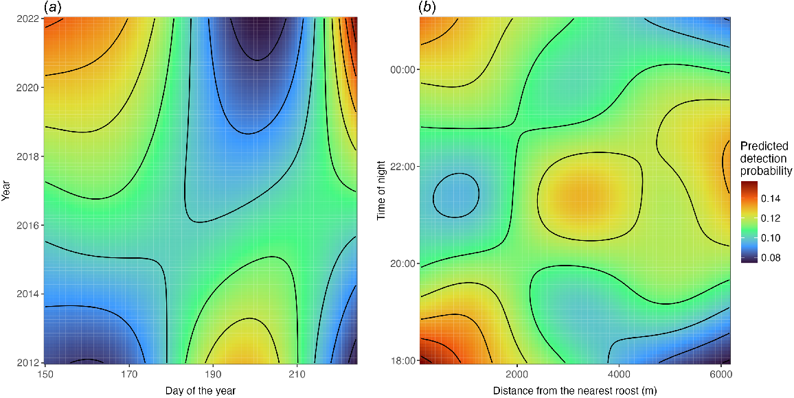
There was also a significant interaction between year and day of the year (Table 3, Fig. 5a). Specifically, although detection probabilities exhibited seasonal patterns within each year, these patterns differed across years. In earlier years, there was a peak in detection probability in the middle of the study period, ~Day 200 from 2012 to 2015, However, in more recent years, detection probability was high at the beginning and the end of the study period (~Day 150 and ~Day 230), with a low detection probability at approximately Day 200 (Fig. 5a). Including data from 2006 did not change these patterns, but showed a higher detection probability in 2006 than in any of the following survey years, similar as shown in Fig. 4.
Predicted detection probability of Pteropus natalis as a function of (a) the interaction between year and day of the year, and (b) time of night and distance from the roost. Shown are the predicted probabilities, with the intercept added to account for baseline detection probabilities.
The effect of the vegetation type, as represented by the NMDS axes, also changed with year. In 2012, sites with a higher value for NMDS2 and a lower value for NMDS1 had higher detection probabilities (Fig. S2). These NMDS values are associated with closed-canopy evergreen forest. These values are also associated with rehabilitation fields and perennial wetland forests, but these had a low R2 (Table 2). The pattern gradually switched, with 2022 having higher detection probabilities for sites with high scores for NMDS1 and low scores for NMDS2 (Fig. S2), which is associated with semi-deciduous scrub, semi-deciduous forest, coastal fringe vegetation, regrowth, and weed dominated vegetation and pioneer regrowth (Table 2).
There was a significant interaction between distance from the roost and time of night on detection probability (Table 3, Fig. 5b). At the start of the night, at 18:00 hours, P. natalis detection probability was high near the roost and decreased with an increasing distance from the roost. This trend was inversed later in the night; by approximately 22:00 hours, detection probability was low near the roost, and higher farther away. After midnight, this pattern shifted again, resembling the initial trend (Fig. 5b).
Detection probability significantly decreased with an increasing wind speed (Table 3). The decrease was substantial; when wind speed was 0 on the Beaufort scale [0–0.2 m/s], the predicted detection probability was 0.125, whereas as wind speed increased to 6 [10.8–13.8 m/s], the probability decreased to 0.065, a 48% decrease (Fig. 6a). Detection probability had a significant non-linear relation with distance from the coast (Table 3), with detection probability being high near the coast, at 0.14, and lowest at 1700 m from the coast, at 0.076, and high again at 3000 m from the coast at 0.15 (Fig. 6b). There was also a significant negative effect of time on the detection probability of P. natalis (Table 3), with detection probability decreasing from approximately 0.115 at 18:00:00 hours, to 0.084 at 00:00:00 hours (Fig. 6c), for a total decrease of 27% in detection probability.
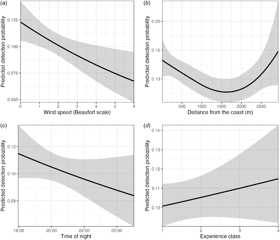
The model indicated that detection probability increased with an increasing experience level (Fig. 6d). Observers with an experience level of ‘1’ had an estimated detection probability of 0.100, whereas those with a higher experience level of ‘4’ had an estimated detection probability of 0.115, an increase of 15%. To assess further whether there was a difference in detection probability between observers in 2022, we made density graphs of the distances of P. natalis detections (Fig. 7). Most of Observer B’s detections were of P. natalis less than 100 m away, with a few detections 100–200 m away, and a single detection 400 m away. In contrast, Observer A detected more P. natalis in the 200–400-m distance (Fig. 7). There was a significant difference in the distribution of detection distances between Observer A, who had intimate experience with P. natalis, and B, who was unexperienced (two-sample Kolmogorov–Smirnov, P = 0.043). Observer B’s density graph was more similar to Observer C’s (2019 observer, experienced, but not with P. natalis) density graph. Interestingly, just over half (52%) of Observer C’s observations were visual, whereas visual observations constituted only 0.04% of Observer B’s observations.

The variable importance analysis demonstrated that, aside from the random effect of site, distance from the coast was the most influential variable for model accuracy (Fig. S3A). This was supported by the hierarchical partitioning analysis, which showed that distance from the coast had the highest individual contribution to the model explained variance (4.3%, Table 4). Year and time were also identified as critical variables, contributing 3.64% and 3.15% respectively, to the model performance. In contrast, experience class, day of the year and NMDS2 contributed the least to model accuracy and had low unique contributions (<1.6%) in the hierarchical partitioning (Table 4).
| Variable/term | Absolute bias | Relative bias (%) | Unique contribution | Relative contribution (%) | |
|---|---|---|---|---|---|
| Year | −2.28 × 10¹⁶ | −2.865 | 0.001 | 1.08 | |
| Day of the year | −4.09 × 10¹⁶ | −1.468 | |||
| Wind | −7.06 × 10¹⁶ | −1.387 | 0.004 | 3.15 | |
| Time | −1.08 × 10¹⁵ | −1.009 | 0.001 | 1.08 | |
| NMDS | −6.75 × 10¹⁶ | −0.723 | |||
| Distance from the roost | −4.12 × 10¹⁶ | −0.709 | |||
| Distance from the coast | −1.85 × 10¹⁶ | −0.408 | 0.005 | 4.30 | |
| Experience class | −4.22 × 10¹⁶ | 0.029 | 0.001 | 0.91 | |
| Year × day of the year | 0.004 | 3.64 | |||
| Year × NMDS | 0.002 | 1.57 | |||
| Distance from the roost × time | 0.005 | 4.3 |
A subsequent bias analysis confirmed that no variable had a significant impact on predictive performance (Table 4). Notably, although distance from the coast was ranked highly in the variable importance analysis, it showed minimal absolute and relative bias. Year displayed the highest relative bias, indicating that temporal trends were more sensitive to the exclusion of this variable. The plot of model performance with and without year clearly illustrates how temporal trends are captured only when year is included (Fig. S3F). Wind speed also showed a large bias (Table 4), and excluding it altered detection patterns (Fig. S3D). Although time, day of the year, and distance from the coast had higher relative biases than did other variables (Table 4), their exclusion did not substantially change detection trends (Fig. S3B, C, E).
Discussion
In this study, we explored factors affecting detection probability of P. natalis, to improve current monitoring efforts and interpretability for this critically endangered insular species. We found that year, time of night, and distance from the coast were key drivers of detection patterns. Our findings showed that P. natalis detection probability varied significantly with year, and its interactions with day of the year, and vegetation types. At both the start and the end of the night, P. natalis was more likely to be detected closer to the roost. Detection probability also was higher on calmer nights, earlier in the night, and with an increasing distance from the coast, although this trend reversed at greater distances inland. Furthermore, observer experience significantly affected detection probability. Importantly, analyses that excluded environmental and spatiotemporal variables suggested a modest increase in detections since 2012. However, once these variables were incorporated, no such trend was found; instead, a decrease in detection probability was indicated in between 2019 and 2022. These results highlight the importance of accounting for environmental and spatiotemporal variables, which aid in accurate interpretation of survey data.
Detection probability changed significantly over the years, increasing between 2012 and 2018, followed by a decrease. However, the significant change appears only in 2020. This suggests that whereas there were fluctuations in detection probability over time, these shifts were small, with the only pronounced change occurring in 2020. This pattern could indicate that detection probability is stable overall, despite the dip observed in 2020. However, the decrease since 2018 is noteworthy and warrants close and ongoing scrutiny, because it could potentially reflect a decline in the P. natalis population. Notably, a different trend was shown through the methods historically used for this survey, namely, mean incidence scores (Woinarski et al. 2014; Schulz 2019). Even though the mean incidence scores showed a decrease between 2019 and 2022, they generally suggested an upward trend. This contrast highlights the importance of more robust analyses that account for spatiotemporal and environmental variables, enabling a clearer isolation of the effect of year on the detection probability.
Temporal changes in foraging patterns are also likely to affect detection probability of P. natalis over the survey period, because spatiotemporal changes in foraging resource distribution could affect aggregation patterns of P. natalis. When P. natalis is more aggregated, detection probability could either be lower, because bats are found only in a few locations, or higher because the bats could be vocalising more because of a higher likelihood of interactions. Indeed, detection probability varied with day of the year, but the pattern depended on the survey year. In earlier survey years, the detection probability was higher in the middle of the survey period, whereas in more recent years, the detection probability was higher at the start and the end of the survey period. Changes in bat foraging patterns are common (Funakoshi et al. 1991; Fahr et al. 2015; Czenze et al. 2018; Conenna et al. 2019), and for flying-foxes they are highly dependent on the phenology of foraging resource trees (Eby 1991). A foraging resource that could attract large numbers of bats might have been available in the middle of the survey period in earlier years, causing larger aggregations resulting in increased intraspecific interactions and thus vocalisations. A change in the phenology or availability of those resources could have led to a change in detection probability as a result.
The possibility that spatiotemporal dynamics in foraging resource distribution affect detection probability is also suggested by the change in vegetation types used over the years. In earlier years, P. natalis was more likely to be detected in areas with closed-canopy evergreen forest, forest rehabilitation fields, and perennial wetland forests. This pattern gradually shifted in later years, with higher detection probabilities in semi-deciduous scrub, semi-deciduous forest, and coastal fringe vegetation. Pteropus alecto has been shown to move through the landscape following flowering and fruiting of certain plant species (Palmer et al. 2000), and the change in use of vegetation types could reflect that some vegetation types provided more foraging resources in some years than in others. In coastal fringe and semi-deciduous forest areas where P. natalis was more likely to be detected in recent years, species such as Pandanus christmatensis and Erythrina variegata are dominant species. Pollen of these species was frequently found on P. natalis during 2015–2018 (Todd 2019), indicating that these species provide critical resources from June to October and may have been drivers of detection probability for P. natalis in recent survey years. In contrast, detection probability in wetlands was higher during earlier survey years, potentially reflecting recent changes in the phenology of Inocarpus fagifer, a crucial wetland foraging resource for P. natalis (Todd 2019; Pulscher et al. 2021). Similarly, closed-canopy evergreen forest, characterised by species such as Planchonella nitida and Syzygium nervosum, with pollen found on P. natalis from 2015 to 2017 (Todd 2019), also showed decreased detection probability in recent years, possibly indicating shifts in dietary preferences or resource availability. Further research into the phenology of key plant species and factors affecting their fruiting and flowering could provide critical insights into the spatiotemporal dynamics of P. natalis habitat use.
Detection also generally decreased with an increase in day of the year. This can possibly be attributed to slight changes in phenology of Inocarpus fagifer, a tree species that is highly prevalent in and restricted to the island’s wetlands and is an important foraging resource to P. natalis (Todd 2019; Pulscher et al. 2021). The fruits of I. fagifer are thought to be primarily eaten from January to July. Although the survey period overlaps with the tail end of this fruiting window, recent shifts in phenology could have resulted in reduced fruit availability in June and July, potentially explaining the lower detection probability in this vegetation type in recent years. Detection probability was also higher in closed-canopy evergreen forest during earlier survey years. This vegetation type is characterised by species such as Planchonella nitida and Syzygium nervosum, from which pollen was found on P. natalis between 2015 and 2017 (Todd 2019). However, detection probability in this vegetation type has decreased in recent years, again reflecting a potential shift in dietary preference or resource availability. Further research into phenology of key plant species, as well as factors affecting fruiting and flowering timing and success, could provide critical insights into the temporal dynamics of P. natalis habitat use.
Other factors
Pteropus natalis had a higher probability of detection closer to established roost sites early in the night, approximately 18:00 hours, with detection probability decreasing as the distance from the roost increased. This pattern corresponds to the initial foraging behaviour of P. natalis, because individuals emerge and begin foraging in nearby areas before dispersing further away. This behaviour is consistent with central place foraging theory, where energy demands prompt feeding close to the roost, before dispersing (Pyke et al. 1977; Stephens and Krebs 1986). By 22:00 hours, detection probability was highest further away from the roost sites, indicating that P. natalis may gradually move away from the roost sites when foraging, potentially seeking more abundant or higher-quality resources at greater distances. After midnight, the pattern reverted to higher detection probabilities near the roost, potentially reflecting the return of individuals to their roost sites as they conclude foraging bouts. Alternatively, they may continue foraging closer to the roost or even fly out again after a brief return. However, because surveys did not continue beyond 01:00 hours, we cannot confirm this. One study on P. poliocephalus found that males returned to their mating territories earlier in the night (between 22:00 hours and 00:00 hours) during the mating season (Welbergen 2011). The sampling period for the present study overlaps with P. natalis mating season (Todd et al. 2018), and the increased detection probability near the roost site towards midnight could similarly reflect the return of dominant males. Another study of P. poliocephalus also found higher detection probabilities near the roost site (McDonald-Madden et al. 2005). However, this study did not include time of night as a factor, so it could have overlooked potential shifts in spatial foraging patterns over the course of the night. The temporal pattern shown in our study suggests that P. natalis adopts a dynamic foraging strategy, adjusting its spatial use of the landscape in response to changing energetic needs throughout the night. Notably, because of the small size of the island, P. natalis has a limited maximum straight-line foraging distance of 15 km, compared with other Pteropus species that regularly forage much further away from their roost (Eby 1991; Palmer and Woinarski 1999; Banack and Grant 2002; Meade et al. 2021; Yabsley et al. 2021). However, P. natalis still exhibits strategic foraging behaviour by first foraging near the roost site and gradually moving further away over the night, likely optimising energy expenditure. These findings underscore the importance of accounting for the spatiotemporal dynamics of foraging habitat utilisation in flying-fox monitoring programs.
Pteropus natalis was more likely to be detected on calm nights. This is in accordance with a previous study conducted in 2012, in which Woinarski et al. (2014) observed that removing samples affected by wind exceeding 4 on the Beaufort scale [5.5–7.9 m/s] led to a slight increase in detection probability for P. natalis. Wind has also been found to affect acoustic detection probability in birds (Thomas et al. 2020; Jahn et al. 2022) and other bat species (Perks and Goodenough 2020). In contrast, rain did not affect detection probability of P. natalis, which was also found in previous research (Woinarski et al. 2014). However, surveys were not conducted during heavy rain, and the model does not account for broader environmental factors, such as the annual rainfall patterns. Such broad environmental factors could have influenced detection probabilities. Weather patterns are known to influence the availability of foraging resources (Morellet et al. 2013; Lisovski et al. 2017), leading to spatiotemporal fluctuations in resource availability among years. This variability in resource availability might explain the differences in spatial distribution and distribution index of P. natalis detections observed across different years.
Pteropus natalis has previously been shown to forage predominantly near the coast and near roost sites during the dry season (Dorrestein 2023). Our study corroborated this finding by demonstrating an increased detection probability near the coast and a higher detection probability in areas with a greater extent of coastal fringe vegetation. However, the majority of sampling sites are still positioned far away from the coastline for observers to robustly detect P. natalis foraging very close to the shore. Coastal foraging resource availability can vary, and in years when resources are more abundant near the coast, bats may gather in areas that are not well covered by the current survey network, leading to a reduced detection probability. Increasing the number of sampling sites closer to the coastline could help address this potential issue, especially because P. natalis is much more likely to be detected near the coast.
Time of night and day of the year affected P. natalis detection probability. The effect of time of night could indicate a change in P. natalis activity patterns, as has been found in other bat species (Perks and Goodenough 2020). It has been suggested that interspecific resource partitioning could lead to differences in bat activity patterns (Perks and Goodenough 2020). However, there are no other frugivorous or nectarivorous nocturnal animals on Christmas Island and, therefore, interspecific resource partitioning pattern does not occur. The change in detection probability could also indicate an increase in observer fatigue during the night, or a heightened ability to visually detect individuals closer to sunset because of the higher light levels. Future surveys could focus solely on the first 4–5 h of the night. However, this would increase the number of survey days required, because the number of samples would have to spread out over a larger number of days. Alternatively, by including time of night in the analysis, this effect is accounted for and so should not affect the interpretation of results.
Observer bias
Observer experience also affected the detection probability, which has been regularly found in other studies (Lotz and Allen 2007; Fitzpatrick et al. 2009; Bernard et al. 2013). All observers followed the same approach, but experience differed among observers. Detection probability increased substantially with an increase in experience level. Because this assigned experience level was an approximation, we assessed observer bias in more detail for 2022, when two observers with contrasting experience were used. Observer A, with extensive knowledge of P. natalis and its vocalisations, had a substantially higher detection rate than did Observer B, who had never worked with P. natalis before. This difference highlights the importance of experience in both aural and visual detections. At the sampling sites, visual detection of P. natalis is often limited to approximately 50 m because of dense vegetation, whereas we estimated that aural detection to extend up to 400 m under favourable conditions. Experienced observers, such as Observer A, are more adept both at recognising P. natalis vocalisation from a distance and at visually identifying the bats, even under challenging conditions, such as spotlighting or recognising their silhouette in flight. Observer B’s density graph was similar to that of Observer C, 2019 observer, who had a lot of experience with flying-fox surveys, but not with P. natalis specifically. This similarity between the patterns of detection with distance by Observer B and C could mean that the mean detection determined by Observer A is an outlier, indicating that the 2022 mean detection might be lower than reported. Furthermore, Observer B’s lower visual detection further underscores the importance of experience in these surveys. In other studies, it has also been shown, in both flora and fauna surveys, that experienced individuals are more likely to detect small populations, or rare individuals (e.g. Fitzpatrick et al. 2009; Jeffress et al. 2011; Shirley et al. 2012). Overall, it is likely that fluctuations in recorded detection probability are, at least in part, the result of differences in observer experience, and although its effect on model accuracy is low, excluding the variable from analyses could lead to subtle, yet critical, shifts in detection probability estimates.
Variable importance
The variable importance analysis showed that distance from the coast was the most influential predictor in determining detection probability, indicating a key role in shaping habitat-use patterns of P. natalis. This finding aligns with results from GPS tracking data, where P. natalis was often located in coastal areas (Dorrestein 2023), possibly owing to resource availability or roosting sites closer to the coast. Year also emerged as a critical variable, with both high relative bias and unique contributions in the hierarchical partitioning, underscoring the importance of temporal variation in detection probability. This finding suggests potential shifts in environmental conditions over time, or changing population dynamics. Other variables had lower contributions to model accuracy and minimal unique contributions, suggesting that although these variables affect detection probability, their effects are more subtle, or become evident through interactions with other factors. Overall, the analyses suggest that distance from the coast and year have a particularly important effect on P. natalis detection, and are critical to include in future analyses.
Conclusions
In conclusion, our study showed that incorporating environmental and spatiotemporal variables through generalised additive models indicates a more nuanced and accurate understanding of the species’ detection probability and more detailed and accurate insights into population trajectory. Our study did not incorporate long-term environmental variables, such as the effect of yearly rain patterns on foraging resource availability, but it is likely that such factors could play a role in spatiotemporal variability in detection of the species as well. Our findings can help improve the monitoring design for P. natalis, and other species worldwide. We showed that it is crucial to include all vegetation types when designing a monitoring program, because foraging preferences or foraging resource availability may change over time. Additionally, when sampling is conducted under varying environmental conditions, and at different times of night or year, it is important to account for these factors in the analyses. It is essential that sample sizes are sufficient to account for each factor, because consideration of the impact of these factors was possible only because of the large sample size. Hence, attempts to reduce investments in monitoring through a smaller sample size may compromise interpretability of the results. However, survey efforts could be focussed on times when detection probabilities are higher, such as calm nights, or earlier in the evening. This could maximise detection probability, and consequently reduce the required survey effort. Similarly, it may be important to minimise the number of observers involved and, ideally, maintain consistency in observers between surveys, with a preference for observers with more experience to maximise detection probability. Further, including statistical modelling that accounts for environmental and spatiotemporal factors in assessing survey results will provide more accurate estimates of detection probability and prevent misinterpretation. Our findings contribute to a more robust understanding of the factors affecting P. natalis detection probability, provide avenues to maximise survey effectiveness and emphasise the importance of employing comprehensive methods that account for environmental and spatiotemporal factors affecting detection probability of a highly mobile, critically endangered species.
Data availability
The data used in this study is the property of the Director of National Parks, Australia.
Acknowledgements
We are grateful to all the staff of Christmas Island National Park and others who have conducted and supported the survey of P. natalis since 2006. We also thank Christmas Island Phosphates for enabling access to survey sites on mining leases. Thanks also go to Rosie Willacy and Kristen Schubert for providing comments on a draft of the initial report from which this paper developed. This research was conducted under a Commonwealth contract, in compliance with environmental laws and the Christmas Island National Park Management Plan, allowing for research activities with minimal impact on the studied species.
References
Australian Bureau of Meteorology (2021) Weather data Christmas Island 1995–2021. Available at http://www.bom.gov.au/climate/dwo/IDCJDW6026.latest.shtml
Banack SA, Grant GS (2002) Spatial and temporal movement patterns of the flying fox, Pteropus tonganus, in American Samoa. The Journal of Wildlife Management 66(4), 1154-1163.
| Crossref | Google Scholar |
Bernard ATF, Götz A, Kerwath SE, Wilke CG (2013) Observer bias and detection probability in underwater visual census of fish assemblages measured with independent double-observers. Journal of Experimental Marine Biology and Ecology 443, 75-84.
| Crossref | Google Scholar |
Clarke KR (1993) Non-parametric multivariate analyses of changes in community structure. Australian Journal of Ecology 18(1), 117-143.
| Crossref | Google Scholar |
Conenna I, López-Baucells A, Rocha R, Ripperger S, Cabeza M (2019) Movement seasonality in a desert-dwelling bat revealed by miniature GPS loggers. Movement ecology 7(1), 27.
| Crossref | Google Scholar |
Czenze ZJ, Tucker JL, Clare EL, Littlefair JE, Hemprich-Bennett D, Oliveira HFM, Mark Brigham R, Hickey AJR, Parsons S (2018) Spatiotemporal and demographic variation in the diet of New Zealand lesser short-tailed bats (Mystacina tuberculata). Ecology and Evolution 8(15), 7599-7610.
| Crossref | Google Scholar | PubMed |
Eby P (1991) Seasonal movements of grey-headed flying-foxes, Pteropus poliocephalus (Chiroptera: Pteropodidae), from two maternity camps in northern New South Wales. Wildlife Research 18(5), 547-559.
| Crossref | Google Scholar |
Erwin RM (1982) Observer variability in estimating numbers: an experiment. Journal of Field Ornithology 53(2), 159-167.
| Google Scholar |
Fahr J, Abedi-Lartey M, Esch T, Machwitz M, Suu-Ire R, Wikelski M, Dechmann DKN (2015) Pronounced seasonal changes in the movement ecology of a highly gregarious central-place forager, the African straw-coloured fruit bat (Eidolon helvum). PLoS ONE 10(10), e0138985.
| Crossref | Google Scholar | PubMed |
Fitzpatrick MC, Preisser EL, Ellison AM, Elkinton JS (2009) Observer bias and the detection of low-density populations. Ecological Applications 19(7), 1673-1679.
| Crossref | Google Scholar | PubMed |
Forsyth DM, Scroggie MP, McDonald-Madden E (2006) Accuracy and precision of grey-headed Flying-fox (Pteropus poliocephalus) flyour counts. Wildlife Research 33, 57-65.
| Crossref | Google Scholar |
Funakoshi K, Kunisaki T, Watanabe H (1991) Seasonal changes in activity of the northern Ryukyu fruit bat Pteropus dasymallus dasymallus. Journal of the Mammalogical Society of Japan 16(1), 13-25.
| Google Scholar |
Greenwell BM, Boehmke BC (2020) Variable importance plots: an introduction to the vip package. The R Journal 12(1), 343-366.
| Crossref | Google Scholar |
Hayes JP (1997) Temporal variation in activity of bats and the design of echolocation-monitoring studies. Journal of Mammalogy 78(2), 514-524.
| Crossref | Google Scholar |
Hurvich CM, Tsai C-L (1989) Regression and time series model selection in small samples. Biometrika 76(2), 297-307.
| Crossref | Google Scholar |
Jahn P, Ross JG, MacKenzie DI, Molles LE (2022) Acoustic monitoring and occupancy analysis: cost-effective tools in reintroduction programmes for roroa-great spotted kiwi. New Zealand Journal of Ecology 46(1), 3466.
| Crossref | Google Scholar |
James DJ, Dale GJ, Retallick K, Orchard K (2007) Christmas Island flying-fox Pteropus natalis Thomas 1887: an assessment of conservation status and threats. Parks Australia North Christmas Island Biodiversity Monitoring Programme. Report to Department of Finance & Administration and the Department of Environment & Water Resources, Canberra, ACT, Australia. pp. 19–23.
Jeffress MR, Paukert CP, Sandercock BK, Gipson PS (2011) Factors affecting detectability of river otters during sign surveys. The Journal of Wildlife Management 75(1), 144-150.
| Crossref | Google Scholar |
Lai J, Tang J, Li T, Zhang A, Mao L (2024) Evaluating the relative importance of predictors in generalized additive models using the gam.hp R package. Plant Diversity 46, 542-546.
| Crossref | Google Scholar |
Lisovski S, Ramenofsky M, Wingfield JC (2017) Defining the degree of seasonality and its significance for future research. Integrative and Comparative Biology 57(5), 934-942.
| Crossref | Google Scholar | PubMed |
Lotz A, Allen CR (2007) Observer bias in anuran call surveys. The Journal of Wildlife Management 71(2), 675-679.
| Crossref | Google Scholar |
Marsh DM, Trenham PC (2008) Current trends in plant and animal population monitoring. Conservation Biology 22(3), 647-655.
| Crossref | Google Scholar | PubMed |
McCarthy ED, Martin JM, Boer MM, Welbergen JA (2022) Ground-based counting methods underestimate true numbers of a threatened colonial mammal: an evaluation using drone-based thermal surveys as a reference. Wildlife Research 50, 484-493.
| Crossref | Google Scholar |
McDonald-Madden E, Schreiber ESG, Forsyth DM, Choquenot D, Clancy TF (2005) Factors affecting grey-headed Flying-fox (Pteropus poliocephalus: Pteropodidae) foraging in the Melbourne metropolitan area, Australia. Austral Ecology 30(5), 600-608.
| Crossref | Google Scholar |
Meade J, Martin JM, Welbergen JA (2021) Fast food in the city? Nomadic flying-foxes commute less and hang around for longer in urban areas. Behavioral Ecology 32(6), 1151-1162.
| Crossref | Google Scholar |
Morellet N, Bonenfant C, Börger L, Ossi F, Cagnacci F, Heurich M, Kjellander P, Linnell JDC, Nicoloso S, Urbano F, Mysterud A, Sustr P (2013) Seasonality, weather and climate affect home range size in roe deer across a wide latitudinal gradient within Europe. Journal of Animal Ecology 82(6), 1326-1339.
| Crossref | Google Scholar | PubMed |
Oedin M, Brescia F, Boissenin M, Vidal E, Cassan J-J, Hurlin J-C, Millon A (2019) Monitoring hunted species of cultural significance: estimates of trends, population sizes and harvesting rates of flying-fox (Pteropus sp.) in New Caledonia. PLoS ONE 14(12), e0224466.
| Crossref | Google Scholar | PubMed |
Otto MC, Pollock KH (1990) Size bias in line transect sampling: a field test. Biometrics 46, 239-245.
| Crossref | Google Scholar |
Padgham M, Lovelace R, Salmon M, Rudis B (2017) osmdata. Journal of Open Source Software 2, 305.
| Crossref | Google Scholar |
Palmer C, Woinarski JCZ (1999) Seasonal roosts and foraging movements of the black flying fox (Pteropus alecto) in the Northern Territory: resource tracking in a landscape mosaic. Wildlife Research 26(6), 823-838.
| Crossref | Google Scholar |
Palmer C, Price O, Bach C (2000) Foraging ecology of the black flying fox (Pteropus alecto) in the seasonal tropics of the Northern Territory, Australia. Wildlife Research 27(2), 169-178.
| Crossref | Google Scholar |
Pebesma E (2018) Simple features for R: standardized support for spatial vector data. The R Journal 10, 439-446.
| Crossref | Google Scholar |
Perks SJ, Goodenough AE (2020) Abiotic and spatiotemporal factors affect activity of European bat species and have implications for detectability for acoustic surveys. Wildlife Biology 2020(2), 1-8.
| Crossref | Google Scholar |
Pulscher LA, Dierenfeld ES, Welbergen JA, Rose KA, Phalen DN (2021) A comparison of nutritional value of native and alien food plants for a critically endangered island flying-fox. PLoS ONE 16(5), e0250857.
| Crossref | Google Scholar | PubMed |
Pyke GH, Pulliam HR, Charnov EL (1977) Optimal foraging: a selective review of theory and tests. The Quarterly Review of Biology 52(2), 137-154.
| Crossref | Google Scholar |
R Core Team (2021) ‘R: a language and environment for statistical computing.’ (R Foundation for Statistical Computing: Vienna, Austria) Available at http://www.R-project.org/
Reddiex B, Forsyth DM, McDonald-Madden E, Einoder LD, Griffioen PA, Chick RR, Robley AJ (2006) Control of pest mammals for biodiversity protection in Australia. I. Patterns of control and monitoring. Wildlife Research 33(8), 691-709.
| Crossref | Google Scholar |
Reddy S, Dávalos LM (2003) Geographical sampling bias and its implications for conservation priorities in Africa. Journal of Biogeography 30(11), 1719-1727.
| Crossref | Google Scholar |
RStudio Team (2020) ‘RStudio: Integrated Development for R.’ (RStudio, Inc.: Boston, MA, USA). Available at www.rstudio.com
Shirley MH, Dorazio RM, Abassery E, Elhady AA, Mekki MS, Asran HH (2012) A sampling design and model for estimating abundance of Nile crocodiles while accounting for heterogeneity of detectability of multiple observers. The Journal of Wildlife Management 76(5), 966-975.
| Crossref | Google Scholar |
Thomas A, Speldewinde P, Roberts JD, Burbidge AH, Comer S (2020) If a bird calls, will we detect it? Factors that can influence the detectability of calls on automated recording units in field conditions. Emu – Austral Ornithology 120(3), 239-248.
| Crossref | Google Scholar |
Tidemann CR, Yorkston HD, Russack AJ (1994) The diet of cats, Felis catus, on Christmas Island, Indian Ocean. Wildlife Research 21, 279-286.
| Crossref | Google Scholar |
Todd CM, Westcott DA, Rose K, Martin JM, Welbergen JA (2018) Slow growth and delayed maturation in a Critically Endangered insular flying fox (Pteropus natalis). Journal of Mammalogy 99(6), 1510-1521.
| Crossref | Google Scholar | PubMed |
Utzurrijm RCB, Wiles GJ, Brooke AP, Worthington DJ (2003) Count methods and population trends in Pacific island flying-foxes. In ‘Monitoring trends in bat populations of the United States and territories: problems and prospects’. (Eds TJ O’Shea, MA Bogan) pp. 49–61. US Geological Survey, Biological Resources Division, Information and Technology Report, Washington, USA.
Vincenot CE, Florens FV, Kingston T (2017) Can we protect island flying foxes? Science 355(6332), 1368-1370.
| Crossref | Google Scholar | PubMed |
Wagner JL (1981) Visibility and bias in avian foraging data. The Condor 83(3), 263-264.
| Crossref | Google Scholar |
Walker K, Porritt K, Sexton M (2014) Christmas Island Vegetation and Clearing Dataset. Geoscience Australia, Canberra, ACT, Australia. Available at http://pid.geoscience.gov.au/dataset/ga/82430
Welbergen JA (2011) Fit females and fat polygynous males: seasonal body mass changes in the grey-headed flying fox. Oecologia 165(3), 629-637.
| Crossref | Google Scholar | PubMed |
Westcott DA, McKeown A (2004) Observer error in exit counts of flying-foxes (Pteropus spp.). Wildlife Research 31(5), 551-558.
| Crossref | Google Scholar |
Westcott DA, Fletcher CS, McKeown A, Murphy HT (2012) Assessment of monitoring power for highly mobile vertebrates. Ecological Applications 22(1), 374-383.
| Crossref | Google Scholar | PubMed |
Winiarska D, Szymański P, Osiejuk TS (2024) Detection ranges of forest bird vocalisations: guidelines for passive acoustic monitoring. Scientific Reports 14(1), 894.
| Crossref | Google Scholar | PubMed |
Woinarski JCZ, Flakus S, James DJ, Tiernan B, Dale GJ, Detto T (2014) An Island-wide monitoring program demonstrates decline in reporting rate for the Christmas Island Flying-Fox Pteropus melanotus natalis. Acta Chiropterologica 16, 117-127.
| Crossref | Google Scholar |
Wood SN (2011) Fast stable restricted maximum likelihood and marginal likelihood estimation of semiparametric generalized linear models. Journal of the Royal Statistical Society: Series B 73(1), 3-36.
| Crossref | Google Scholar |
Yabsley SH, Meade J, Martin JM, Welbergen JA (2021) Human-modified landscapes provide key foraging areas for a threatened flying mammal: the grey-headed flying-fox. PLoS ONE 16(11), e0259395.
| Crossref | Google Scholar | PubMed |