
Habitat use of invasive chital deer is associated with soil mineral content
Catherine L. Kelly A B * , Lin Schwarzkopf A , Iain J. Gordon C D E , Anthony Pople F and Ben T. Hirsch A G
A
B
C
D
E
F
G
Abstract
Ungulates have been introduced to many environments around the world. Some of these populations have become invasive, resulting in severe economic, social, and environmental impacts. In 1886, chital deer (Axis axis) were introduced to north Queensland, Australia, and the population has since grown and expanded.
To understand where chital deer are likely to occur in the future, we examined the relationship between chital deer abundance and environmental variables at two scales, namely, local and regional.
The local scale was surveyed using camera traps on a single property, and regional scale data were collected from a landholder survey of properties across the current distribution of chital deer in the region.
High predicted soil phosphorus was correlated with high relative abundance of chital deer at both the local and regional scales. In addition, at the local scale, higher predicted soil sodium content and normalised vegetation index (NDVI, ‘greenness’), close proximity to homesteads and highways, and lower canopy cover and height were strongly correlated with increased chital deer abundance.
There were more chital in areas with high predicted soil phosphorus at both local and regional scales.
This study has the following two implications for management: (1) areas with high predicted soil phosphorous content had the highest relative abundance of deer at both scales, and should be the focus of control efforts, and (2) such areas are more vulnerable to future invasion of chital deer and should be monitored closely.
Keywords: Australia, cervid, control, invasive species, management, phosphorus, soil minerals, ungulate.
Introduction
Ungulates have been introduced and successfully established worldwide, usually as food or game resources (Mungall and Sheffield 1994; Forsyth and Hickling 1998; Moriarty 2004; Ikagawa 2013; Hess 2016; King and Forsyth 2021). Some of these introduced ungulate populations have negative economic and social impacts, causing damage to infrastructure Oxford, motor vehicle collisions, and competing with livestock for feed (Côté et al. 2004; Dolman and Wäber 2008; Kušta et al. 2017). Invasive ungulates can cause serious environmental effects by degrading habitats, competing with native species, and spreading diseases or parasites (Doran and Laffan 2005; Ens et al. 2016; Hess 2016). Control of invasive ungulates to effectively mitigate their impacts requires an understanding of how they behave in their environment.
Ungulate habitat selection is often determined by factors such as the availability of water, essential minerals, forage, and shelter (Grasman and Hellgren 1993; Smit et al. 2007; Treydte et al. 2009; Thaker et al. 2011). Local-scale habitat selection can then scale up to influence larger-scale patterns of a species’ distribution. Various geographic barriers can also heavily influence the distribution of a species across a landscape (Hobbs 2003, Northrup et al. 2016). In the context of invasive species, different environmental features can facilitate or inhibit spread in a novel range (With 2002). For these reasons, understanding the drivers of species’ habitat use at multiple scales is important for predicting where species may occur in the future. For example, ungulate habitat selection can be influenced by the availability of minerals in plant material or in the soil as licks (Grasman and Hellgren 1993; Mungall and Sheffield 1994; Ayotte et al. 2006; Treydte et al. 2009; Watter et al. 2019a). Phosphorus and sodium are vital nutrients for bone mineralisation, which is important for antler growth in deer, as well as for subcellular processes and genetic coding (Belovsky 1978; Grasman and Hellgren 1993; Mungall and Sheffield 1994; Dryden 2016; Griffith et al. 2017). Soil mineral content depends on factors such as soil drainage, soil pH, land use, and the original mineral content of the parent material (Shaw et al. 1994; Turner et al. 2007; Huang et al. 2017). Weathering reduces soil phosphorus availability over time, thus geologically older regions, such as continental Australia, typically have phosphorus-deficient soils (Gillman and Bell 1978; McKenzie et al. 2004; Rossel and Bui 2016; Huang et al. 2017; Kooyman et al. 2017). Sodium is also important to ungulates, with salt-deprived individuals having reduced reproduction and survival (Church et al. 1971). Ungulates around the world exhibit high reliance on sodium licks, particularly where soil sodium contents are deficient (Weeks and Kirkpatrick 1976; Moe 1993; Maro and Dudley 2022). For instance, females appear to disproportionately seek out salt licks during periods of lactation (Singer 1978; Atwood and Weeks 2002; Ayotte 2004). Soil mineral content may thus influence invasive ungulate habitat selection and spread through a landscape.
Chital deer (also known as axis or spotted deer, Axis axis; hereafter referred to as chital) are a medium-sized cervid native to India, Sri Lanka, Bangladesh, and Nepal (Mattioli 2011). They have been introduced to many countries including the United States (Texas, Hawaii, and Maryland), Argentina, Chile, Croatia, and Australia (Long 2003). In their native range, chital usually inhabit forest edges in grassland and riverine environments (Mishra 1982; Moe and Wegge 1994). Chital habitat use can also be influenced by the presence of native predators such as tigers (Panthera tigris), leopards (Panthera pardus), jackals (Canis aureus), and dhole (Cuon alpinus; Moe and Wegge 1994; Sankar and Acharya 2004; Ramesh et al. 2012). Chital respond to predation risk by using open grass areas for grazing and then retreating to dense vegetation for resting or cover (Mishra 1982; Moe and Wegge 1994). Because habitat selection in their native range is strongly influenced by predators, examining habitat use in an introduced population with fewer predators could show other factors important to their distribution.
In 1886, four chital were introduced to north Queensland, Australia, and subsequently established and spread (Bentley 1967; Moriarty 2004). Following establishment, chital exhibited a lag in population growth (Kelly et al. 2021). Up to 20 years ago, the north Queensland chital population had remained localised, but the population is currently expanding rapidly, which is a concern to local landowners and government authorities (Forsyth et al. 2019; Kelly et al. 2021). The factors that have facilitated (or inhibited) their spread in north Queensland are poorly understood. This complicates targeting management efforts to prevent spread. Understanding the habitat selection of chital in their introduced range should help determine how and where such populations might grow and spread in the future.
Previous studies undertaken on the local scale have identified several factors that may contribute to chital habitat use or range expansion in northern Queensland. Forsyth et al. (2019) found higher chital numbers close to water and homesteads, whereas Watter et al. (2019a) stressed the importance of soil minerals because of seasonal changes in dietary plant selection. We built on these previous studies by investigating chital abundance in relation to multiple habitat variables at both local and regional scales. Because deer elsewhere avoid anthropogenic features, such as tracks and roads (Scholten et al. 2018), we expected the relative abundance of chital to increase with increasing distance from these features. We also expected that areas with high soil phosphorus, close proximity to water, and with more green vegetation should have more chital, because these factors are all important nutritionally (Watter et al. 2019a). We expected that these relationships would also be reflected at the regional scale (i.e. high soil phosphorus, close proximity to water, and higher normalised vegetation index (NDVI) would correlate with increased chital relative abundance).
Materials and methods
Local scale
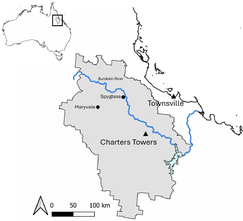
This study was conducted at Spyglass Beef Research Facility, a cattle property covering 38,221 ha in the Charters Towers district, Queensland, Australia (Fig. 1). The study area contains grassland consisting of both native and exotic grasses, such as black speargrass (Heteropogon contortus), kangaroo grass (Themeda triandra), sabi grass (Urochloa mosanbicensis), red Natal grass (Melinis repens), and buffel grass (Cenchrus ciliaris). A variety of overstorey species including silverleaf box (Eucalyptus pruinosis), lancewood (Acacia shirleyi), bendee (Acacia catenulata), yellowjacket (Eucalyptus similis), and ironbark (Eucalyptus spp.) make up the canopy. Three main seasons are experienced at the study site, namely, wet (November–April), cool dry (May–August), and hot dry (September–October). Troughs and dams are located across Spyglass as permanent water sources for cattle. The Burdekin River runs adjacent to the north-eastern edge of Spyglass and may also serve as a permanent water source for animals. There are three homesteads in the study area, two on Spyglass itself and one on a neighbouring property close to the boundary. As a working cattle property, mineral supplementation (including phosphorus) is provided, although the locations of these blocks were unknown. No additional broad-scale phosphorus (i.e. fertiliser) is applied on this property.
Location of broad (Charters Towers district) and fine scale (Spyglass Beef Research Station) areas investigated to determine the factors that drive the distribution of invasive chital deer in north Queensland.
We used camera traps to determine the presence and relative abundance of chital in different habitats (Supplementary material Fig. S1). To select camera trap locations, a grid with points 500 m apart was created using ArcGIS (ESRI) (actual average distance between points: 554.14 m). To facilitate access to the locations, 118 points of the grid were selected that fell within 400 m of a road or track. Bushnell Aggressor™ cameras were placed at these locations for at least 1 month each between October 2017 and November 2018. Cameras were set to capture three images per trigger, with no delay between consecutive triggers. All images were stamped with the date and time. Cameras were installed approximately 30–50 cm above the ground and pointed north or south to avoid the rising or setting sun. Vegetation in front of the cameras was clipped to minimise interference and false triggers. Of the 118 cameras installed, 24 failed, or the data they collected could not be analysed (e.g., they collected excessive false triggers; Supplementary material Table S1), resulting in 94 operational cameras, representing 6707 trap days. Images were identified and organised using WildID and ZSL CTap software (TEAM Network 2011; Amin et al 2015).
For analysis, an ‘event’ was defined as a sequence of photographs of one species that occurred following a previous sequence of a different species. When there were consecutive events of the same species, we ensured there was 1 h or more between events (Bowkett et al. 2008; Amin et al. 2015; Rovero et al. 2017). This time frame was used to avoid repeated counting of the same individuals (Tobler et al. 2009; Rovero et al. 2017; Bruce et al. 2018). We used Moran’s test in ArcGIS to compare the detection rates of chital across all cameras and found no significant spatial autocorrelation in our dataset (Moran’s index: 0.09, P = 0.313).
We calculated spatial covariates for each camera site by using geoprocessing tools in ArcGIS (Table 1), including distance to homesteads, distance to tracks and highways, distance to the nearest water sources (dams, troughs, or the Burdekin River), foliage projective cover, and the average predicted mineral concentrations (phosphorus, sodium, and calcium:magnesium ratios; all surface (0–0.1 m) depth) within the 100-m radius of each camera. Predicted mineral concentrations were extracted from maps (phosphorus: Department of Environment and Science 2023; sodium: Department of Environment and Science 2016a; calcium:magnesium: Department of Environment and Science 2016b). In brief, the phosphorus map was created by modelling relationships between point measurements of mineral contents and environmental covariate data, the sodium and calcium–magnesium maps were created on the basis of the methods of Rayment and Lyons (2011), based on soil pH and method uncertainty, by using multiple methods (exchangeable cations, Mehlich 3 extractable elements, and MIR reflectance spectroscopy). Details for how each map was generated can be found in their respective metadata, and sources for all data used and details for how each map was generated can be found in Table 1. An average NDVI (a measure of vegetation greenness; Pettorelli 2014) was derived for a 250-m radius around each camera site by using MoveBank’s Moderate Resolution Imaging Spectroradiometer (MODIS) Land V6 product (Wikelski et al. 2020). The NDVI for each site (calculated as the 16-day average for the period each camera was active) was automatically calculated and downloaded. To investigate whether predicted soil sodium concentration influenced plant growth, we performed linear regressions between NDVI and average predicted site sodium concentration.
| Variable name | Variable description | Source | |
|---|---|---|---|
| FPC | Foliage predictive cover (%) | Long Paddock (Zhang and Carter 2018) | |
| Canopy height | Approximate average canopy height (m) | Measured at site | |
| NDVI | 16-day average NDVI measure for each site | Moderate Resolution Imaging Spectroradiometer (MODIS) Land V6 product (Wikelski et al. 2020) | |
| Homestead | Log10 distance from the nearest homestead (m) | Measured from local maps | |
| Highway | Log10 distance from the nearest highway (m) | Measured from local maps | |
| Track | Log10 distance from nearest track (m) | Measured from local maps | |
| Water | Log10 distance from nearest permanent water source (m) | Measured from local maps | |
| Dingo | Index of relative abundance of dingoes per site ((events per days active) × 100) | Measured from cameras | |
| P | Phosphorus content of the soil surface (0–0.5 m depth; pixel size: 90 m × 90 m) | Phosphorus map of Queensland (Department of Environment and Science 2023) | |
| Na | Exchangeable sodium concentration of the soil surface (Mg ha−2) (0–0.5 m depth pixel size: 100 m × 100 m) | Queensland digital soil attributes – Burdekin River basin – exchangeable sodium (Department of Environment and Science 2016a) | |
| Ca:Mg | Ratio of calcium:magnesium content of soil (0–0.5 m depth; pixel size: 100 m × 100 m) | Queensland digital soil attributes – Burdekin River basin – Ca:Mg ratio (Department of Environment and Science 2016b) |
We used a generalised linear model (GLM) to model relative chital abundance as a function of spatial covariates across the 94 camera sites. Prior to analyses, all variables were checked for collinearity (Table S2) and scaled using the scale () function in the glmmTMB package (ver. 1.1.9; https://cran.r-project.org/web/packages/glmmTMB/index.html; Brooks et al. 2017) that centres and scales predictor variables (Brooks et al. 1998). Our analyses were based on counts (the number of chital photo events at each site). To avoid overdispersion and account for the excess zeros in our data, we used a negative binomial distribution (Lambert 1992; Zuur et al. 2009). The zero-inflated model was constructed using the glmmTMB package that allows for offset variables (Brooks et al. 1998) where effort (the number of days the camera was operating) was included as an offset. We used Akaike’s information criterion (AICc) to select the best models of habitat selection. Following model selection, the residuals were checked to avoid overdispersion by using the DHARMa package (ver. 0.4.6; https://cran.r-project.org/web/packages/DHARMa/index.html; Hartig 2022; Fig. S2). We calculated delta AICc values (model AICc – minimum AICc), where models with delta AICc values of <2 were considered most plausible (Burnham and Anderson 2002; Symonds and Moussalli 2011). All analyses were conducted in R (ver. 4.4.1; R Core Team 2024) and visualised using the ggplot2 package (ver. 3.5.1; https://cran.r-project.org/web/packages/ggplot2/index.html; Wickham 2016).
Regional scale
To examine larger-scale patterns of chital abundance, we used a survey of landowners (Supplementary material File S1). Surveys (n = 254) were distributed by the Charters Towers Regional Council over 2018–2019. Landholders were asked to estimate the number of chital on their property either as a numerical or categorical estimate (0, 1–50, 51–200, 201–1000, >1000). Where a categorical estimate was provided, the lower end of the estimate was used (i.e. if the estimate was 51–200, 51 was used for analyses). Property boundaries were derived from property boundary maps supplied by Charters Towers Regional Council, and polygons for each respondent property were created in ArcMap. Chital estimates per property were calculated by dividing the minimum population estimate by the size of the property, thus resulting in a minimum estimated population density for each property that returned a survey. Properties outside the potential range of this chital population were excluded from the analyses, which were defined as properties that fell more than 50 km beyond two consecutive properties that reported no deer.
A number of potential predictors of chital abundance at the regional scale were considered. These predictor layers, as well as the sources of all data used, are available in Table 2. As water availability is likely to influence chital landscape use, we calculated the distance from the nearest major watercourse (i.e. those classified by Geoscience Australia 250,000 Topographic Data as being majo (Department of Resources 2023) to the geometric centre of each property. This was selected over other possible estimates of water availability, because we did not have locations where chital were sighted. All properties have dams and troughs that provide permanent water to cattle. Average predicted soil mineral concentration (Mg ha−1) of phosphorus, and sodium, and the ratio of calcium:magnesium were calculated for each property. Similar to the local scale analyses, we know mineral supplementation was provided on properties, but its extent was not quantified. Because of the climate in this region, broad-scale phosphorus fertilisers are not widely used (on the basis of discussions with landholders). The average NDVI (average of a 10-year dataset to estimate average station greenness) was also calculated for each property and used as a covariate. To determine whether the average predicted soil sodium content influenced plant growth, we looked for significant linear regressions between NDVI and average property predicted sodium concentration. Because of the potential impact of predators, landholders were also asked whether they undertook dog control on the property; however, not every landholder responded to this question. Of the 84 properties that responded, 54 (68%) answered the dog control question. Of those, 100% responded that they undertook dog control. As such, whether landholders employed dog control on their property was excluded as a potential predictor from analyses.
| Variable name | Variable description | Source | |
|---|---|---|---|
| River | Average distance from a major watercourse (m) | Measured from: major watercourse lines – Queensland (Department of Resources 2023) | |
| NDVI | 10-year average NDVI measure for each property | Moderate Resolution Imaging Spectroradiometer (MODIS) Land V6 product (Wikelski et al. 2020) | |
| P | Average phosphorus concentration of soil (Mg ha−1) | Phosphorus map of Queensland (Department of Environment and Science 2023) | |
| Na | Average exchangeable sodium concentration of soil (Mg ha−1) | Queensland digital soil attributes – Burdekin River basin – exchangeable sodium (Department of Environment and Science 2016a) | |
| Ca:Mg | Average ratio of calcium:magnesium content of soil | Queensland digital soil attributes – Burdekin River basin – Ca:Mg ratio (Department of Environment and Science 2016b) | |
| Slope | Average slope of a property | Measured from: 3-second Digital Elevation Model (Department of Resources 2013) |
GLMs were used to investigate predictors of chital abundance per property. Prior to analyses, all variables were checked to ensure that collinearity did not exceed a threshold of 0.75 (Table S3). To avoid overdispersion and account for the excess zeros in our data, we used a negative binomial distribution. We used count data (the number of chital reported on each property) with property area included as an offset. All variables were scaled prior to model selection by using the scale () function in the glmmTMB package (Brooks et al. 2017), as with local level analyses. As with the local scale analyses, we calculated delta AICc values where models with delta AICc values of <2 were considered most plausible (Burnham and Anderson 2002; Symonds and Moussalli 2011), and the residuals were checked to avoid overdispersion (Fig. S3). Model averaging was performed when no single best model could be identified (i.e. multiple models with a ΔAICc value of <2). All analyses were conducted in R (ver. 4.4.1; R Core Team 2024) and visualised using the ggplot2 package (Wickham 2016).
Ethics
All procedures performed in studies involving human participants were in accordance with the ethical standards of the institutional and/or national research committee and with the 1964 Helsinki declaration and its later amendments or comparable ethical standards. The template and methodology for this survey was approved by the Human Ethics Committee of James Cook University (Approval number: H7666).
Results
Local scale
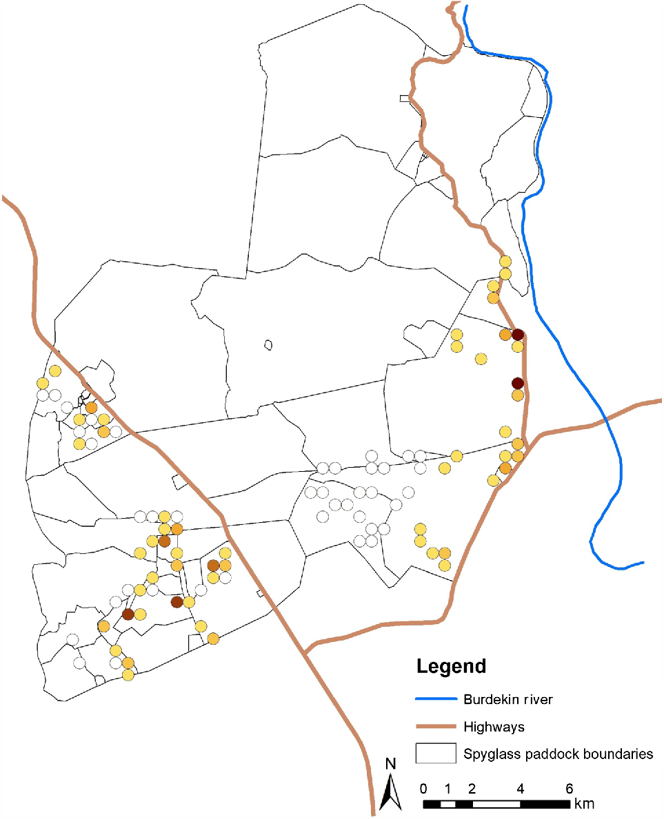
Cameras recorded an average of 7.96 (±1.73 s.e.) chital events, or 0.14 (±0.03 s.e.) per day (Fig. 2). In total, 753 chital events were recorded across all camera sites. At the local scale, there were two plausible models (Table S4), so model averaging was performed. Parameter estimates are given in Table 3.
Map of chital trapping densities at cameras on Spyglass Beef Research Station. Open symbols represent sites where chital were absent, with increasingly dark solid symbols representing increasing chital trapping rate <0.00–1.34 events per day (each shade darker represents an increase in trapping rate of 0.224 events per day).
| Item | Estimate | s.e. | Adjusted s.e. | z-value | 2.50% | 97.50% | P-value | |
|---|---|---|---|---|---|---|---|---|
| Intercept | −2.83 | 0.20 | 0.20 | 14.00 | −3.23 | −2.44 | 0.00 | |
| Canopy height | −0.54 | 0.16 | 0.16 | 3.36 | −0.85 | −0.22 | 0.00 | |
| Homestead | −0.38 | 0.16 | 0.16 | 2.32 | −0.70 | −0.06 | 0.02 | |
| Highway | −0.62 | 0.16 | 0.16 | 3.87 | −0.93 | −0.30 | 0.00 | |
| Track | −0.29 | 0.14 | 0.14 | 2.05 | −0.58 | −0.01 | 0.04 | |
| FPC | −0.58 | 0.17 | 0.17 | 3.33 | −0.92 | −0.24 | 0.00 | |
| Na | 0.51 | 0.16 | 0.16 | 3.09 | 0.19 | 0.83 | 0.00 | |
| NDVI | 0.45 | 0.16 | 0.16 | 2.78 | 0.13 | 0.77 | 0.01 | |
| P | 0.36 | 0.14 | 0.14 | 2.60 | 0.09 | 0.63 | 0.01 |
All models include effort (days that the camera was active) as an offset variable.
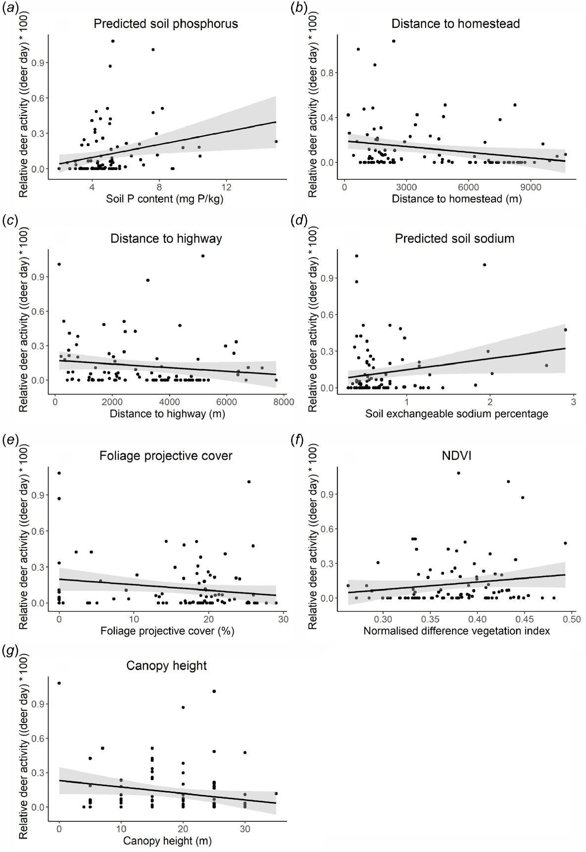
The relative abundance of chital increased closer to homesteads (estimate = −0.38; 95% CI (−0.70 – −0.06); Fig. 3) and highways (estimate = −0.62; 95% CI (−0.93 – −0.30)) and tracks (estimate = −0.29; 95% CI (−0.58 – −0.01)), increased with an increasing predicted soil phosphorus (estimate = 0.36; 95% CI (0.09–0.63)), sodium (estimate = 0.51; 95% CI (0.19–0.83)), and NDVI (estimate = 0.45; 95% CI (0.13–0.77)), but decreased with increasing foliage projective cover (estimate = −0.58; 95% CI (−0.92 – −0.24)), and canopy height (estimate = −0.54; 95% CI (−0.85 – −0.22)). There was no significant relationship between chital abundance and dingo abundance measured by cameras, or between chital abundance and proximity to permanent water points. There was also no significant relationship between average predicted site soil sodium content and NDVI (P = 0.858).
Relationship between the ‘trapping rate’ of chital deer at a local scale determined from trail cameras (estimated as deer events per day) and (a) predicted soil phosphorus content (mg P kg−1), (b) distance from nearest homestead (m), (c) distance from nearest highway (m), (d) predicted soil sodium content (Mg ha−1), (e) foliage projective cover (FPC; %), (f) normalised difference vegetation index (NDVI), and (g) canopy height (m).
Regional scale
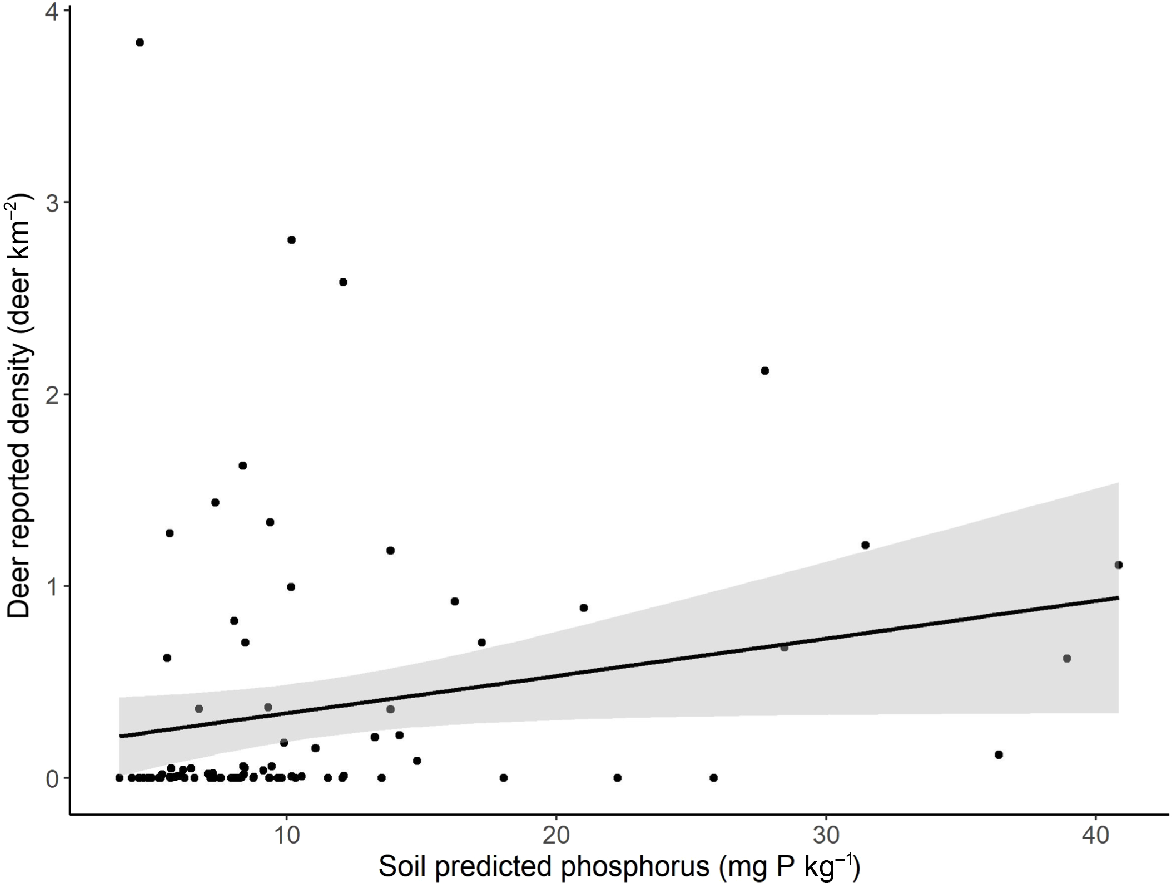
Of 98 returned surveys (38.58% response rate), 56 reported chital on their property, ranging from 1 to 2000 individuals, and an average of 0.64 chital km−2 (±0.12 s.e.). At the regional scale, there were 18 plausible models following model selection (Table S5), so model averaging was performed. Parameter estimates are given in Table 4.
| Item | Estimate | s.e. | Adjusted s.e. | z-value | 2.50% | 97.50% | P-value | |
|---|---|---|---|---|---|---|---|---|
| Intercept | −0.80 | 0.26 | 0.27 | 3.00 | −1.33 | −0.28 | 0.00 | |
| P | 0.42 | 0.12 | 0.12 | 3.52 | 0.19 | 0.65 | 0.00 | |
| Na | −0.13 | 0.17 | 0.18 | 0.73 | −0.58 | 0.10 | 0.46 | |
| River | −0.10 | 0.15 | 0.15 | 0.65 | −0.53 | 0.09 | 0.52 | |
| Slope | −0.13 | 0.21 | 0.21 | 0.63 | −0.75 | 0.15 | 0.53 | |
| NDVI | −0.08 | 0.15 | 0.15 | 0.53 | −0.58 | 0.11 | 0.59 | |
| CaMg | 0.02 | 0.07 | 0.08 | 0.32 | −0.11 | 0.39 | 0.75 |
All models include the area of the property (km2) as an offset variable.
As with the local scale analyses, reported chital density increased with an increasing average predicted station soil phosphorus content (estimate = 0.42; 95% CI (0.19–0.65); Fig. 4). Although all other variables were included in the top models, they had broad confidence intervals that included zero, reflecting conservative model selection by AICc (Crawley 2013).
Discussion
The relative abundance of chital was higher in areas with high predicted phosphorus at both local and regional scales. This observation is similar to those in previous local-scale studies in this area (Watter et al. 2019a). Phosphorus is critical for ungulates (Grasman and Hellgren 1993; Mungall and Sheffield 1994; Dryden 2016) and, in their native range, chital use natural salt licks high in phosphate (Schaller 1967; Moe 1993). In mineralogically deficient environments, ungulates will actively graze in patches of vegetation with higher phosphorus content or use salt licks (McNaughton 1990; Moe 1993; Ayotte et al. 2006; Treydte et al. 2009). The Charters Towers region contains some of the oldest rock formations in Australia. Given that the phosphorus content of rocks decreases over time because of weathering (Gardner 1990), this region is likely to exhibit particularly low phosphorus concentrations. The chital population north of Charters Towers, where the initial individuals were released, is located on an ‘island’ of higher phosphorus in what is generally a low-phosphorus landscape (Fig. 5; Rossel and Bui 2016), and this could feasibly have decreased the ability of chital to spread out of this region (see Kelly et al (2023) for predicted spread).
History of spread of chital deer in the Charters Towers region estimated from landholder surveys. Red point indicates initial release point and red shading is spread after 20 years, orange is spread after 80 years, yellow is spread after 100 years, and pale yellow is spread after 130 years. The black line is the Burdekin River, and the brown underlay layer is soil phosphorus content sourced from State of Queensland, Department of Environment and Science (2023).

NDVI was positively associated with local chital abundance, whereas foliage cover and canopy height were negatively associated. NDVI values are greater in areas with high pasture biomass, as well as in areas with high tree and shrub cover (although these two variables were not correlated; r = 0.36). These results are consistent with chital habitat selection in their native range, where they typically aggregate and forage in grasslands or areas of freshly sprouting grass (Moe and Wegge 1994; Bhat and Rawat 1995; Ramesh et al. 2012). Likewise, introduced chital in Texas (USA) show a preference for areas with grasses and shoots, either in the understorey, or meadows (Mungall and Sheffield 1994). In their native range, using denser cover is thought to be an anti-predator strategy (Mishra 1982; Moe and Wegge 1994). Despite the lack of a significant influence of dingo camera-trapping rates on chital (Forsyth et al. 2019), dingo populations could influence chital behaviour in this region. At the local level, the relative abundance of chital was positively associated with anthropogenic features such as homesteads and highways. It is possible that anthropogenic clearing in the vicinity of highways and homesteads may provide a corridor between denser vegetation and the open grassland favoured by chital. Our results are consistent with those of Forsyth et al. (2019) and Watter et al. (2019a) who both reported higher chital abundance in close proximity to homesteads; both studies suggested that chital were selecting aspects of habitat found closer to homesteads (i.e. flat, high-quality forage and permanent water sources). Locations close to homesteads may also provide protection from predators, such as dingoes that may avoid humans (see Forsyth et al. 2019), although we did not find a correlation between dingo activity and distance to homestead (−0.13; Table S2). Likewise, highways provide clear areas across flat floodplains that may be associated with higher quality forage.
Predicted soil exchangeable sodium was positively related to chital abundance on the local scale. In their native range, chital use natural licks as a source of sodium (Moe 1993), and other studies have found that sodium was positively associated with ungulate abundance (McNaughton 1988; Robbins 2012), including chital in northern Queensland (Watter et al. 2020). Areas converted from woodland to pasture often exhibit increased soil sodium concentrations, which has been attributed to higher evaporation rates than in the original native woodland (Schofield 1992; Thorburn et al. 2002). The Charters Towers district is at a particular risk of increased soil salinity, because tree clearing, which increases salinity, is commonly used as a land management tool to increase pasture area, and thus beef productivity (Williams et al. 1997). Since tropical grasses take up sodium in only small amounts (Weil and Brady 2017), chital may be selecting areas where the higher soil sodium content enables higher uptake by the plants in those areas.
One limitation of this study is the measurement of water dependency in pastoral regions. On the local scale, analyses were undertaken on a property where water points were common and evenly distributed for provisioning cattle. In addition, the cameras were mostly deployed during the wet season, when chital are less constrained by water availability. At the regional level, the landholder survey was unable to capture the distribution of deer in relation to features such as water sources. In their native range, chital predominantly inhabit riverine forest and grassland edges along river courses (Mishra 1982; Moe and Wegge 1994; Bhat and Rawat 1995; Dey 2007). Chital dependence on water has also been reported in their introduced ranges (Graf and Nichols 1966; Mungall and Sheffield 1994; Centore 2016), as well as in Australia (Forsyth et al. 2019; Watter et al. 2019b). Likewise, high mortality occurs during droughts in Queensland (Watter et al. 2019b; Pople et al. 2023). Maps of the potential distribution of chital (estimated using data from this study and previous landholder surveys) indicate that chital spread may be facilitated by the Burdekin River (a permanent and significant water source in the Charters Towers region; Fig. 5; Kelly et al. 2023). In the future, the reliance of chital on these water sources in a water-limited environment will be investigated using the movement data of GPS tagged deer over multiple seasons. It would also be beneficial to use landscape genetic methods to quantify how the Burdekin River and its tributaries may facilitate the spread of chital in this region.
Another limitation of the study is the reliance placed on landholder responses; there could be tendencies to over- or under-estimate densities depending on different landholder perceptions of deer (e.g. Finch and Baxter 2007; Robertson et al. 2017). Although we acknowledge possible error in such subjective estimates, we found a range of plausible relationships between reported chital densities and various habitat features. In the future, aerial surveys on other properties (e.g. Pople et al. 2023) would provide objective abundance data to model relationships with the environment (e.g. density surface models; Miller et al. 2013; Hinton et al. 2022). There is also the potential for survey non-response bias among rural or farming communities (e.g. Barker 1991; Pendleton 1992; TuckerWilliams et al. 2024). Although we did not account for non-response bias here, we did not detect any notable geographic bias in responses, and property owners both with and without chital responded (57.14% reported chital deer on their property). Potential bias was possibly further mitigated by targeted questionnaires aimed at areas lacking responses (n = 7).
The use of soil nutrient maps also represents a potential limitation of our study. Many studies on habitat use estimate soil and plant nutrient concentrations directly (Ben-Shahar and Coe 1992; Güsewell et al. 2005; Merems et al. 2020), whereas we used soil nutrient values estimated from predictive soil nutrient maps. These digitised layers were sourced from the most up-to-date and high-resolution layers available, but it is possible such maps might lack the resolution and ground-truthing required for finer scale analyses of habitat preference, and, in the future, it would be good to analyse samples at each site to more reliably estimate nutrient concentrations. Although low resolution maps could have been the reason for the surprising lack of a relationship between habitat use and water availability, we suggest this may have been a byproduct of the timing of the camera trap deployments. Chital resource requirements, and thus habitat use, are likely to vary season to season. For example, previous studies have found a nutritional bottleneck for grazing animals prior to the start of the wet season in the dry tropics’ rangelands (McLean et al. 1983; Vetter and Bond 2010; Watter et al. 2020). Watter et al. (2020) and Quin et al. (2025) found that chital altered their diet seasonally, depending on what was growing and available at a given time. In the future, more cameras and seasonal replication will further enhance our understanding of chital habitat use and allow further exploration of spatial variation in occupancy over time. As it stands, our results very closely reflect and build on previous studies (e.g. Forsyth et al. 2019; Watter et al. 2019a).
Chital in north Queensland represent an ongoing threat to agriculture and native ecosystems, with estimates of habitat suitability for chital suggesting that this species has the potential to spread much further than its current distribution (Kelly et al. 2023). Here, chital displayed increased use of habitats that had higher predicted soil phosphorus at both regional and local scales, and increased activity at sites with higher predicted soil sodium content, NDVI, close proximity to homesteads and highways, and lower levels of canopy cover and height. Future studies should examine additional features that may facilitate the spread of chital, such as rivers and other water sources, while simultaneously ground-truthing the work performed here with soil and plant composition analyses, thus allowing more confident predictions of chital distribution and, therefore, focus areas for management.
Data availability
The camera trapping dataset generated and analysed during the current study is available from the corresponding author on reasonable request. The survey data are not publicly available as this would violate the human ethics terms and conditions.
Declaration of funding
This paper was partially funded through an ARC Linkage grant to BTH, LS, AP, Dave Forsyth and Jan Strugnell (LP1801000267). We thank Biosecurity Queensland (Department of Agriculture and Fisheries) and JCU for additional support.
Author contributions
C. Kelly, T. Pople and B. Hirsch conceived and designed the methodology and surveys. CK performed the camera trap survey and analysed the data. C. Kelly, L. Schwarzkopf, I. Gordon, T. Pople, and B. Hirsch wrote the paper.
Acknowledgements
We thank James Cook University and the Department of Agriculture and Fisheries for their support. We thank Dave Forsyth for comment on study design, Ashley Blokland from Charters Towers Regional council for assistance with distributing surveys, and the landholders for their cooperation. We also thank Donald McKnight and Ross Alford for help with statistics and coding. We also thank our volunteers, particularly Christine Zirbel, for their invaluable assistance with fieldwork. Manuscript was edited by Caley Editorial Services. We also gratefully acknowledge the constructive comments of two anonymous reviewers.
References
Amin R, Andanje SA, Ogwonka B, Ali AH, Bowkett AE, Omar M, Wacher T (2015) The northern coastal forests of Kenya are nationally and globally important for the conservation of Aders’ duiker Cephalophus adersi and other antelope species. Biodiversity and Conservation 24, 641-658.
| Crossref | Google Scholar |
Atwood T, Weeks H (2002) Sex- and age-specific patterns of mineral lick use by white-tailed deer (Odocoileus virginianus). The American Midland Naturalist 148(2), 289-296.
| Crossref | Google Scholar |
Ayotte JB, Parker KL, Arocena JM, Gillingham MP (2006) Chemical composition of lick soils: functions of soil ingestion by four ungulate species. Journal of Mammalogy 87(5), 878-888.
| Crossref | Google Scholar |
Barker RJ (1991) Nonresponse bias in New Zealand waterfowl harvest surveys. The Journal of Wildlife Management 55(1), 126-131.
| Crossref | Google Scholar |
Belovsky GE (1978) Diet optimization in a generalist herbivore: the moose. Theoretical Population Biology 14(1), 105-134.
| Crossref | Google Scholar | PubMed |
Ben-Shahar R, Coe MJ (1992) The relationships between soil factors, grass nutrients and the foraging behaviour of wildebeest and zebra. Oecologia 90, 422-428.
| Crossref | Google Scholar | PubMed |
Bhat SD, Rawat GS (1995) Habitat use by chital (Axis axis) in Dhaulkhand, Rajaji National Park, India. Tropical Ecology 36(2), 177-189.
| Google Scholar |
Bowkett AE, Rovero F, Marshall AR (2008) The use of camera-trap data to model habitat use by antelope species in the Udzungwa Mountain forests, Tanzania. African Journal of Ecology 46(4), 479-487.
| Crossref | Google Scholar |
Brooks PD, Williams MW, Schmidt SK (1998) Inorganic nitrogen and microbial biomass dynamics before and during spring snowmelt. Biogeochemistry 43, 1-15.
| Crossref | Google Scholar |
Brooks ME, Kristensen K, van Benthem KJ, Magnusson A, Berg CW, Nielsen A, Bolker BM (2017) glmmTMB balances speed and flexibility among packages for zero-inflated generalized linear mixed modeling. The R Journal 9(2), 378-400.
| Crossref | Google Scholar |
Bruce T, Amin R, Wacher T, Fankem O, Ndjassi C, Bata MN, Fowler A, Ndinga H, Olsen D (2018) Using camera trap data to characterize terrestrial larger-bodied mammal communities in different management sectors of the Dja Faunal Reserve, Cameroon. African Journal of Ecology 56(4), 759-776.
| Crossref | Google Scholar |
Côté SD, Rooney TP, Tremblay J-P, Dussault C, Waller DM (2004) Ecological impacts of deer overabundance. Annual Review of Ecology, Evolution, and Systematics 35, 113-147.
| Crossref | Google Scholar |
Department of Environment and Science (2016a) Queensland digital soil attributes – Burdekin River basin – exchangeable sodium. © State of Queensland 2023. Available at https://qldspatial.information.qld.gov.au/catalogue/custom/detail.page?fid={2020407B-16EC-42A5-85B5-FCCA501B5923} [accessed 30 April 2019]
Department of Environment and Science (2016b) Queensland digital soil attributes – Burdekin River basin - Ca-Mg ratio. © State of Queensland 2020. Available at http://qldspatial.information.qld.gov.au/catalogue/custom/detail.page?fid={97583E64-8251-4919- BC95-4CC [accessed 30 April 2019]
Department of Environment and Science (2023) Queensland predicted soil bicarbonate-extractable phosphorus – map (Stage 3)). © State of Queensland (Department of Environment and Science). Available at https://www.publications.qld.gov.au/dataset/phosphorus-map-of-queensland-pmap/resource/1b35e442-03e4-47e3-be14-44aa6360a6ac [accessed 15 March 2024]
Department of Resources (2013) Digital elevation model - 3 second – Queensland. © State of Queensland 2023. Available at https://qldspatial.information.qld.gov.au/catalogue/custom/detail.page?fid={B9675441-577E-49B6-A5C5-FAA6BC4BC14D} [accessed on 29 April 2019]
Department of Resources (2023) Major watercourse lines – Queensland. © State of Queensland 2023. Available at https://qldspatial.information.qld.gov.au/catalogue/custom/detail.page?fid={22EBABD4-8D0F-46AC-9814-0F3375D9E7DA} [accessed 24 February 2020]
Dolman PM, Wäber K (2008) Ecosystem and competition impacts of introduced deer. Wildlife Research 35(3), 202-214.
| Crossref | Google Scholar |
Doran RJ, Laffan SW (2005) Simulating the spatial dynamics of foot and mouth disease outbreaks in feral pigs and livestock in Queensland, Australia, using a susceptible–infected–recovered cellular automata model. Preventive Veterinary Medicine 70(1–2), 133-152.
| Crossref | Google Scholar |
Dryden GML (2016) Nutrition of antler growth in deer. Animal Production Science 56(6), 962-970.
| Crossref | Google Scholar |
Ens EJ, Daniels C, Nelson E, Roy J, Dicon R (2016) Creating multi-functional landscapes: Using exclusion fences to frame feral ungulate management preferences in remote Aboriginal-owned northern Australia. Biological Conservation 197, 235-246.
| Crossref | Google Scholar |
Finch NA, Baxter GS (2007) Oh deer, what can the matter be? Landholder attitudes to deer management in Queensland. Wildlife Research 34(3), 211-217.
| Crossref | Google Scholar |
Forsyth DM, Hickling GJ (1998) Increasing Himalayan tahr and decreasing chamois densities in the eastern Southern Alps, New Zealand: evidence for interspecific competition. Oecologia 113, 377-382.
| Crossref | Google Scholar | PubMed |
Forsyth DM, Pople A, Woodford L, Brennan M, Amos M, Moloney PD, Fanson B, Story G (2019) Landscape-scale effects of homesteads, water, and dingoes on invading chital deer in Australia’s dry tropics. Journal of Mammalogy 100(6), 1954-1965.
| Crossref | Google Scholar |
Gardner LR (1990) The role of rock weathering in the phosphorus budget of terrestrial watersheds. Biogeochemistry 11, 97-110.
| Crossref | Google Scholar |
Gillman GP, Bell LC (1978) Soil solution studies on weathered soils from tropical north Queensland. Australian Journal of Soil Research 16(1), 67-77.
| Crossref | Google Scholar |
Graf W, Nichols L (1966) The axis deer in Hawaii. Journal of the Bombay Natural History Society 63, 630-734.
| Google Scholar |
Grasman BT, Hellgren EC (1993) Phosophorus nutrition in white-tailed deer: nutrient balance, physiological responses, and antler growth. Ecology 74(8), 2279-2296.
| Crossref | Google Scholar |
Griffith DM, Anderson TM, Hamilton III EW (2017) Ungulate grazing drives higher ramet turnover in sodium-adapted Serengeti grasses. Journal of Vegetation Science 28(4), 815-823.
| Crossref | Google Scholar |
Güsewell S, Jewell PL, Edwards PJ (2005) Effects of heterogeneous habitat use by cattle on nutrient availability and litter decomposition in soils of an Alpine pasture. Plant and Soil 268(1–2), 135-149.
| Crossref | Google Scholar |
Hartig F (2022) DHARMa: residual diagnostics for hierarchical (multi-level/mixed) regression models. R package, version 0.4.6. Available at https://CRAN.R-project.org/package=DHARMa
Hess SC (2016) A tour de force by Hawaii’s invasive mammals: establishment, takeover, and ecosystem restoration through eradication. Mammal Study 41(2), 47-60.
| Crossref | Google Scholar |
Hinton JW, Hurst JE, Kramer DW, Stickles JH, Frair JL (2022) A model-based estimate of winter distribution and abundance of white-tailed deer in the Adirondack Park. PLoS ONE 17(8), e0273707.
| Crossref | Google Scholar | PubMed |
Hobbs NT (2003) Challenges and opportunities in integrating ecological knowledge across scales. Forest Ecology and Management 181(1–2), 223-238.
| Crossref | Google Scholar |
Huang L-M, Jia X-X, Zhang G-L, Shao M-A (2017) Soil organic phosphorus transformation during ecosystem development: a review. Plant and Soil 417, 17-42.
| Crossref | Google Scholar |
Ikagawa M (2013) Invasive ungulate policy and conservation in Hawaii. Pacific Conservation Biology 19(4), 270-283.
| Crossref | Google Scholar |
Kelly CL, Schwarzkopf L, Gordon IJ, Hirsch B (2021) Population growth lags in introduced species. Ecology and Evolution 11(9), 4577-4587.
| Crossref | Google Scholar | PubMed |
Kelly CL, Gordon IJ, Schwarzkopf L, Pintor A, Pople A, Hirsch BT (2023) Invasive wild deer exhibit environmental niche shifts in Australia: where to from here? Ecology and Evolution 13(7), e10251.
| Crossref | Google Scholar | PubMed |
Kooyman RM, Laffan SW, Westoby M (2017) The incidence of low phosphorus soils in Australia. Plant and Soil 412, 143-150.
| Crossref | Google Scholar |
Kušta T, Keken Z, Ježek M, Holá M, Šmíd P (2017) The effect of traffic intensity and animal activity on probability of ungulate–vehicle collisions in the Czech Republic. Safety Science 91, 105-113.
| Crossref | Google Scholar |
Lambert D (1992) Zero-inflated poisson regression, with an application to defects in manufacturing. Technometrics 34(1), 1-14.
| Crossref | Google Scholar |
Maro A, Dudley R (2022) Non-random distribution of ungulate salt licks relative to distance from North American oceanic margins. Journal of Biogeography 49(2), 254-260.
| Crossref | Google Scholar |
McLean RW, McCown RL, Little DA, Winter WH, Dance RA (1983) An analysis of cattle live-weight changes on tropical grass pasture during the dry and early wet seasons in northern Australia: 1. The nature of weight changes. The Journal of Agricultural Science 101(1), 17-24.
| Crossref | Google Scholar |
McNaughton SJ (1988) Mineral nutrition and spatial concentrations of African ungulates. Nature 334, 343-345.
| Crossref | Google Scholar | PubMed |
McNaughton SJ (1990) Mineral nutrition and seasonal movements of African migratory ungulates. Nature 345, 613-615.
| Crossref | Google Scholar |
Merems JL, Shipley LA, Levi T, Ruprecht J, Clark DA, Wisdom MJ, Jackson NJ, Stewart KM, Long RA (2020) Nutritional-landscape models link habitat use to condition of mule deer (Odocoileus hemionus). Frontiers in Ecology and Evolution 8, 98.
| Crossref | Google Scholar |
Miller DL, Burt ML, Rexstad EA, Thomas L (2013) Spatial models for distance sampling data: recent developments and future directions. Methods in Ecology and Evolution 4(11), 1001-1010.
| Crossref | Google Scholar |
Moe SR (1993) Mineral content and wildlife use of soil licks in southwestern Nepal. Canadian Journal of Zoology 71(5), 933-936.
| Crossref | Google Scholar |
Moe SR, Wegge P (1994) Spacing behaviour and habitat use of axis deer (Axis axis) in lowland Nepal. Canadian Journal of Zoology 72(10), 1735-1744.
| Crossref | Google Scholar |
Moriarty A (2004) The liberation, distribution, abundance and management of wild deer in Australia. Wildlife Research 31(3), 291-299.
| Crossref | Google Scholar |
Northrup JM, Anderson CR, Jr, Hooten MB, Wittemyer G (2016) Movement reveals scale dependence in habitat selection of a large ungulate. Ecological Applications 26(8), 2746-2757.
| Crossref | Google Scholar |
Pendleton GW (1992) Nonresponse patterns in the Federal Waterfowl Hunter Questionnaire Survey. The Journal of Wildlife Management 56(2), 344-348.
| Crossref | Google Scholar |
Pople A, Amos M, Brennan M (2023) Population dynamics of chital deer (Axis axis) in northern Queensland: effects of drought and culling. Wildlife Research 50(9), 728-745.
| Crossref | Google Scholar |
Quin MJ, Hirsch BT, Schwarzkopf L, Watter K, People A, Strugnall JM (2025) DNA metabarcoding provides new insight into the diet of invasive chital deer (Axis axis) in a tropical savanna landscape. Ecosphere 16(6), e70288.
| Crossref | Google Scholar |
R Core Team (2024) ‘R: a language and environment for statistical computing, version 4.4.1’ (R Foundation for Statistical Computing: Vienna, Austria) Available at https://www.R-project.org/
Ramesh T, Sankar K, Qureshim Q, Kalle R (2012) Group size, sex and age composition of chital (Axis axis) and sambar (Rusa unicolor) in a deciduous habitat of western Ghats. Mammalian Biology 77(1), 53-59.
| Crossref | Google Scholar |
Robertson A, Delahay RJ, Wilson GJ, Vernon IJ, McDonald RA, Judge J (2017) How well do farmers know their badgers? Relating farmer knowledge to ecological survey data. Veterinary Record 180(2), 48.
| Crossref | Google Scholar | PubMed |
Rossel RAV, Bui EN (2016) A new detailed map of total phosphorus stocks in Australian soil. Science of the Total Environment 542, 1040-1049.
| Crossref | Google Scholar |
Rovero F, Owen N, Jones T, Canteri E, Iemma A, Tattoni C (2017) Camera trapping surveys of forest mammal communities in the Eastern Arc Mountains reveal generalized habitat and human disturbance responses. Biodiversity and Conservation 26, 1103-1119.
| Crossref | Google Scholar |
Schofield NJ (1992) Tree planting for dryland salinity control in Australia. Agroforestry Systems 20, 1-23.
| Crossref | Google Scholar |
Scholten J, Moe SR, Hegland SJ (2018) Red deer (Cervus elaphus) avoid mountain biking trails. European Journal of Wildlife Research 64, 8.
| Crossref | Google Scholar |
Shaw R, Brebber L, Ahern C, Weinand M (1994) A review of sodicity and sodic soil behavior in Queensland. Australian Journal of Soil Research 32(2), 143-172.
| Crossref | Google Scholar |
Singer FJ (1978) Behavior of mountain goats in relation to US Highway 2, Glacier National Park, Montana. The Journal of Wildlife Management 42(3), 591-597.
| Crossref | Google Scholar |
Smit IPJ, Grant CC, Devereux BJ (2007) Do artificial waterholes influence the way herbivores use the landscape? Herbivore distribution patterns around rivers and artificial surface water sources in a large African savanna park. Biological Conservation 136, 85-99.
| Crossref | Google Scholar |
Symonds MRE, Moussalli A (2011) A brief guide to model selection, multimodel inference and model averaging in behavioural ecology using Akaike’s information criterion. Behavioral Ecology and Sociobiology 65, 13-21.
| Crossref | Google Scholar |
Thaker M, Vanak AT, Owen CR, Ogden MB, Niemann SM, Slotow R (2011) Minimizing predation risk in a landscape of multiple predators: effects on the spatial distribution of African ungulates. Ecology 92(2), 398-407.
| Crossref | Google Scholar | PubMed |
Thorburn PJ, Gordon IJ, McIntyre S (2002) Soil and water salinity in Queensland: the prospect of ecological sustainability through the implementation of land clearing policy. The Rangeland Journal 24(1), 133-151.
| Crossref | Google Scholar |
Tobler MW, Carrillo-Percastegui SE, Powell G (2009) Habitat use, activity patterns and use of mineral licks by five species of ungulate in south-eastern Peru. Journal of Tropical Ecology 25(3), 261-270.
| Crossref | Google Scholar |
Treydte AC, Heikonig IMA, Ludwig F (2009) Modelling ungulate dependence on higher quality forage under large trees in African savannahs. Basic and Applied Ecology 10(2), 161-169.
| Crossref | Google Scholar |
TuckerWilliams E, Lepczyk CA, Morse W, Smith M (2024) Perceptions of wild pig impact, management, and policy in Alabama. Environmental Management 73(5), 1032-1048.
| Google Scholar |
Turner B, Condron L, Richardson SJ, Peltzer DA, Allison VJ (2007) Soil organic phosphorus transformations during pedogenesis. Ecosystems 10, 1166-1181.
| Crossref | Google Scholar |
Vetter S, Bond WJ (2010) Changing predictors of spatial and temporal variability in stocking rates in a severely degraded communal rangeland. Land Degradation & Development 23(2), 190-199.
| Crossref | Google Scholar |
Watter K, Baxter G, Pople A, Murray PJ (2019a) Effects of wet season mineral nutrition on chital deer distribution in northern Queensland. Wildlife Research 46(6), 499-508.
| Crossref | Google Scholar |
Watter K, Baxter G, Brennan M, Pople A, Murray P (2019b) Decline in body condition and high drought mortality limit the spread of wild chital deer in north-east Queensland, Australia. The Rangeland Journal 41(4), 293-299.
| Crossref | Google Scholar |
Watter K, Baxter G, Brennan M, Pople A, Murray P (2020) Seasonal diet preferences of chital deer in the northern Queensland dry tropics, Australia. The Rangeland Journal 42(3), 211-220.
| Crossref | Google Scholar |
Weeks HP, Jr, Kirkpatrick CM (1976) Adaptations of white-tailed deer to naturally occurring sodium deficiencies. The Journal of Wildlife Management 40(4), 610-625.
| Crossref | Google Scholar |
Wikelski M, Davidson S, Kays R (2020) Movebank: archive, analysis and sharing of animal movement data. Hosted by the Max Planck Institute of Animal Behavior. Available at https://www.movebank.org [accessed 5 May 2020]
Williams J, Bui EN, Gardner E, Littleboy M, Probert ME (1997) Tree clearing and dryland salinity hazard in the Upper Burdekin Catchment of North Queensland. Australian Journal of Soil Research 35(4), 785-802.
| Crossref | Google Scholar |
With KA (2002) The landscape ecology of invasive spread. Conservation Biology 16(5), 1192-1203.
| Crossref | Google Scholar |
Zhang B, Carter J (2018) FORAGE – an online system for generating and delivering property-scale decision support information for grazing land and environmental management. Computers and Electronics in Agriculture 150, 302-311.
| Crossref | Google Scholar |
Zuur A, Ieno E, Walker N, Saveliev A, Smith G (2009) ‘Mixed effects models and extensions in ecology with R. Statistics for Biology and Health.’ (Springer) 10.1007/978-0-387-87458-6_1