
Characterising the seasonal nature of meteorological drought onset and termination across Australia
A. J. Gibson A * , D. C. Verdon-Kidd B and G. R. Hancock B
A Faculty of Science and Engineering, Southern Cross University, Lismore, NSW, Australia.
B School of Environmental and Life Sciences, The University of Newcastle, Callaghan, NSW, Australia.
Journal of Southern Hemisphere Earth Systems Science 72(1) 38-51 https://doi.org/10.1071/ES21009
Submitted: 23 April 2021 Accepted: 28 December 2021 Published: 8 February 2022
© 2022 The Author(s) (or their employer(s)). Published by CSIRO Publishing on behalf of BoM. This is an open access article distributed under the Creative Commons Attribution-NonCommercial-NoDerivatives 4.0 International License (CC BY-NC-ND)
Abstract
Drought, and its associated impacts, represents one of the costliest natural hazards worldwide, highlighting the need for prediction and preparedness. While advancements have been made in monitoring current droughts, prediction of onset and termination have proven to be much more challenging. This is because drought is unlike any other natural hazard and cannot be characterised by a single weather event. There is also a high degree of spatial variability in this phenomenon across the vast expanse of the Australian continent. Therefore, by characterising regionally specific expressions of drought, we may improve drought predictability. In this study, we analyse the timing of onset and termination of meteorological droughts across Australia from 1900 to 2015, as well as their local and regional climate controls. We show that meteorological drought onset has a strong seasonal signature across Australia that varies spatially, whereas termination is less seasonally restricted. Using a Random Forest modelling approach with predictor variables representative of large-scale ocean-atmosphere phenomena and local climate, up to 75% of the variance in the Standardised Precipitation Index during both onset and termination could be explained. This study offers support to continued development in long-lead forecasting of local and large-scale ocean/atmosphere conditions to improve drought prediction in Australia and elsewhere.
Keywords: drought management, drought onset, drought prediction, drought termination, machine learning, meteorological drought, random forest, Standardised Precipitation Index.
1. Introduction
Globally, drought is estimated to cost US$6–8 billion each year in agricultural related losses (Botterill and Cockfield 2013). To reduce this, a need for drought policy to shift away from disaster-relief-based management strategies to ones that promote climate resilience has been identified (Botterill 2003; Pozzi et al. 2013). Such resilience policies encourage preparedness for drought through management plans that conserve resources during dry periods and promote recovery when conditions ease (Pozzi et al. 2013). However, this approach is impeded by the nature of the drought itself. Unlike other natural disasters, drought manifests and sustains itself over a long period of time (months to years) and then terminates abruptly (Verdon-Kidd et al. 2017; Hao et al. 2018). Due to limitations in long-term rainfall forecasting, predicting meteorological drought is difficult (van Dijk et al. 2013; Kiem et al. 2016; Hao et al. 2018). For resilience-based drought management strategies to be effective, this needs to be improved.
A variety of methods have been investigated to improve drought predictability. Studies have used remotely sensed water storage products and biophysical indicators to build skilled lead time on drought prediction (Pozzi et al. 2013; Tian et al. 2019), and combined indicator approaches are widely used to monitor drought risk across the globe (Pozzi et al. 2013). However, these take an ‘impact’ approach to observe what is happening in response to drying conditions, rather than forecasting the meteorological conditions that either cause or break a drought. A promising method that may provide this missing link is using the state of ocean-atmosphere climate drivers and local climate variables to develop statistical models and relationships with rainfall anomalies and drought indices (van Dijk et al. 2013; Deo and Sahin 2015a, 2015b; Mera et al. 2018; Liu et al. 2019). This relies on an adequate understanding of the regional drought characteristics and the host of potential climate influences specific to that region.
Further complicating the prediction of meteorological droughts are the various definitions used to identify events. Many operational definitions are subjective and quantitative definitions based on indices or direct measures of rainfall (Quiring 2009; Kiem et al. 2016). These can also vary greatly between regions (Quiring 2009). For example, for the commonly used Standardised Precipitation Index (SPI), the definitions for drought proposed by McKee et al. (1993) define drought as occurring at SPI < −1, with severity increasing as SPI decreases. Quiring (2009) showed that, for Texas, the categories of McKee et al. (1993) underestimated the severity of drought and they would not be suitable operational definitions for triggering a timely drought response. The concepts of drought onset and termination then further complicate this, making it difficult to capture trends during these periods (i.e. how long does a precipitation deficit need to be sustained? Is a return to near normal drought termination or is it a return to wetness?). As a result, the effect of drought definition needs to be considered when looking at historical trends in drought and drought prediction.
Building on previous applications of developing statistical models to predict SPI, this study aims to determine how much variability in the SPI during meteorological drought onset and termination can be explained using a suite of local and regional climate indices. To achieve this, we first characterised geographical seasonal bias in the timing of drought onset and termination across Australia. The impact of drought definition on drought records is also explored. This is achieved by applying the SPI to rainfall records at 14 locations across Australia. We use two definitions for drought termination and compare these results. The need for region-specific approaches to improve prediction is demonstrated by determining the contribution of Australian climate drivers to drought onset and termination through a Random Forest approach. We take a novel approach to understanding drought in the Australian context by only looking at trends in SPI over drought onset and termination. In doing so, this study aims to identify an opportunity for better drought prediction by characterising the drivers responsible for starting and ending Australian droughts.
2. Methods and data
2.1. Defining drought
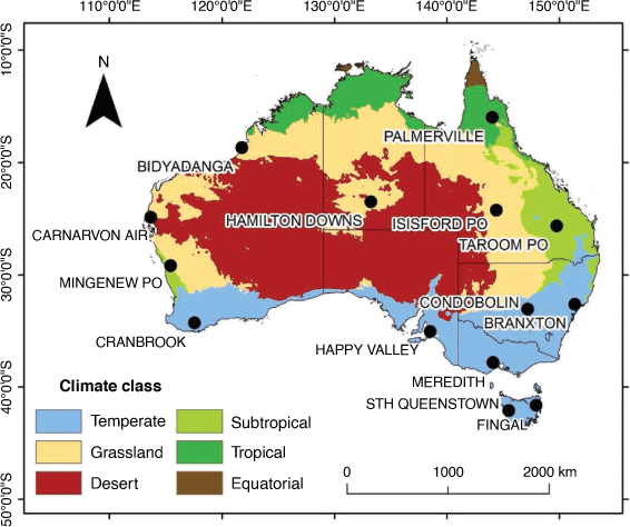
Rainfall data was sourced from the Australian Bureau of Meteorology’s High-Quality Climate Change Datasets (Lavery et al. 1997). For a meteorological station to be included in the analyses, complete, monthly data from 1900 to 2015 was required. Fourteen stations were selected, covering Australia’s major climate zones (Fig. 1). To test if these stations were representative of the surrounding area, observed data was regressed against SILO gridded rainfall data (Jeffrey et al. 2001). An average from the pixel the station was located in and the surrounding 8 pixels (i.e. a 3 × 3 grid) was calculated for use in the regression. Coefficients of determination ranged from 0.85 to 1, with root mean square error values ranging from 2.2 to 14.77 mm. As a result, the station data was deemed representative.
|
The 6-months Standardised Precipitation Index (SPI6) was calculated at each location to create a monthly drought record spanning 1900–2015. The SPI6 was chosen to represent drought in this study to constrain the focus to persistent meteorological droughts. Such droughts extend across multiple seasons, impacting soil and surface water availability, with associated widespread economic and social impacts (e.g. The Millennium Drought) (van Dijk et al. 2013; Verdon-Kidd et al. 2017; Hao et al. 2018; Gibson et al. 2020). The SPI is based on rainfall alone, which provides the opportunity to assess the contribution of temperature to drought statistics as an independent variable. This is opposed to indices, such as the Palmer Drought Severity Index (PDSI) or the Standardised Precipitation Evapotranspiration Index (SPEI), which require temperature for evaporation calculations.
The SPI6 represents the number of standard deviations 6-monthly totals of rainfall depart from the mean using a gamma transformation. This is calculated at monthly timesteps, with positive values indicating wet conditions, and negative values indicating dry conditions (McKee et al. 1993, 1995). Individual drought periods were defined as six or more consecutive months where SPI6 values were below −1 (moderate drought); with the first of these months identified as the onset month (month 0). Two definitions of drought termination were used (Dettinger 2013). One record was generated where droughts were deemed to have ended when there were six or more consecutive months of SPI6 > −1 (near normal to mild drought; McKee et al. 1993), and the second record was generated where droughts were considered to terminate after six consecutive months of SPI6 > 0 (near normal to slightly wet; McKee et al. 1993). Similar to onset, the first month where SPI exceeded the threshold value in the string of six was identified as the month of termination (month 0). Where a single month was defined as the onset or termination month, it is important to note that this represents a cumulative effect of rainfall on the SPI during the 6 months preceding. The season (i.e. spring, summer, autumn, winter) when each drought period identified in the record officially began and ended was collated for each station.
2.2. Drivers of drought onset and termination
Timeseries of local weather variables and climate indices representing large-scale climate drivers were compared with the SPI6 during the 6 months prior to and 6 months after drought onset and termination. This approach was selected, as opposed to predicting whole-record rainfall anomalies (e.g. van Dijk et al. 2013; Deo et al. 2017), to narrow the focus to drought onset and termination specifically. Eight variables representing the major large-scale drivers known to influence Australian rainfall (Risbey et al. 2009) were used (data sources outlined in Table 1). Local temperature and monthly mean sea level pressure (MSLP) were also included as measures of the role of local conditions in drought onset and termination.

|
A Random Forest approach was adopted to model SPI6 using the state of the indices during drought onset and termination. By determining the best combination of drivers for modelling SPI6 during drought onset and termination, the importance of each driver could then be quantified. This method was selected, as it allowed for relationships to be identified between SPI and the climate drivers during drought onset and termination (Deo et al. 2017; Feng et al. 2019). This approach also allowed the relative importance of each variable to be calculated using permutation importance. Random Forest modelling does not assume independence of observations, only that the bagging of samples for model development is representative, allowing numerous drivers to be used and capturing the effect of teleconnections (Breiman 2001). Here, the Random Forest regressor function in the scikit-learn python package was used (Pedregosa et al. 2011).
Three key parameters of Random Forest modelling are (1) the number of trees used in the forest (ntree), (2) the minimum number of samples in a terminal node (nodesize) and (3) the minimum number of variables available for splitting at each node (Mtry). The model was trained on 66% of the months in the onset and termination datasets and then tested using the remaining months (due to the varying number of droughts at each location, this ranged from a total of 35–91 months available; see Table 2 for number of droughts). To define the parameters, out of bag error scores were used, with these stabilising where ntree was 100 and nodesize and Mtry were 2. For prediction of monthly SPI6 (i.e. the response variable), this process was repeated using monthly and 6-months rolling averages of each variable (to match the timescale of the SPI6). It was found that the 6-months averaged data was better able to predict SPI6, believed to be due to the reduced noise in higher frequency indices, such as the Southern Annular Mode (SAM). The final results were then generated using these parameters and 6-months averages for the climate variables, with a separate model built for both onset and termination at each station.

|
Variable importance was calculated to determine the most significant drivers of drought onset and termination at each station (following a similar approach to Van Dijk et al. (2013) and Deo and Sahin (2015b)). This was done by calculating the permutation importance for variables in the training and test data. Importance was calculated for the training and test data to avoid giving inflated importance due to overfitting and to better align the results with the total variance explained at each location. Variables were iteratively interchanged out of the model 10 times, and the mean decrease in model score (R2 in this study) was reported as the variable importance. The overall aim of this was to quantify the contribution of local and regional drivers to drought onset and termination and their seasonality, rather than to predict drought.
3. Results
3.1. Number of droughts and drought run-length
For droughts defined using a termination threshold of −1, all stations recorded between 9 and 14 droughts (Table 2). Average run-lengths were close to 10 months for all stations (using the –1 termination threshold; Table 2), with the longest drought lasting 21 months (Table 2). The record using a 0 termination threshold of reduces the number of droughts, with these ranging from 5 to 13 droughts (Table 2). Average run-lengths increased, ranging from 13 to 25 months (Table 2), with 84 months being the longest recorded drought. Average drought severity did not show any spatial pattern and increased from the SPI6 −1 termination threshold record to the 0 termination threshold record, due to the inclusion of months with higher SPI6 (not reported).
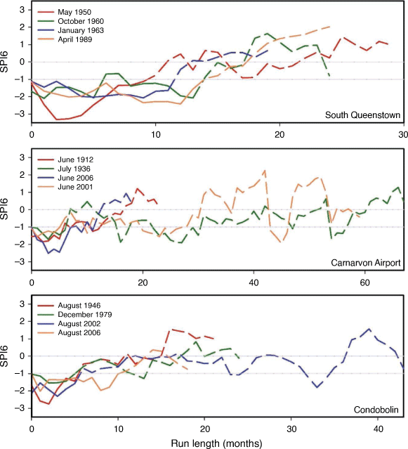
The variations in droughts using the two different termination definitions can be broken into four broad categories (Fig. 2). The first of these is no change, where the droughts identified cross the two thresholds in the same month and maintain sustained wetness. The second is a slight extension of drought by 1–6 months with the end of drought closely followed by a return to ‘wet’ conditions (e.g. the 1963 and 1989 droughts at South Queenstown in Fig. 2). The third category is a persistent extension of drought conditions, whereby multiple shorter droughts from the −1 threshold record merge together when using the 0 threshold. These droughts represent multi-year protracted drought periods (e.g. The WWII drought shown by the 1936 drought event at Carnarvon in Fig. 2) and are characterised by periods of SPI6 < −1, and returns to periods of SPI6 < 0, but lack sustained periods of wetness (SPI > 0). The final category is a lengthy extension of the drought period but no merging of droughts from the −1 threshold record (e.g. the 2002 drought at Condobolin in Fig. 2). These are similar to the third category, again representing a lack of SPI6 above 0. At most stations the extended droughts can be observed, while the central southern stations exhibit more of the shorter extensions of drought as indicated by the mean differences in run-lengths (Table 2).
|
3.2. Timing of drought onset and termination
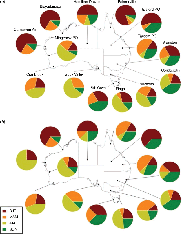
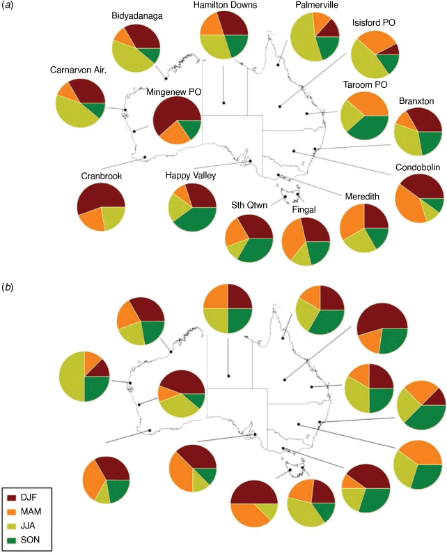
For the record using −1 as the termination threshold, stations located in the northern half of Australia display a clear summer dominant pattern of drought onset (Fig. 3a). Stations in the southwest corner display an autumn–winter-based onset, transitioning to a winter–spring onset for the central south and along the east coast (Fig. 3a). The timing of drought onset for the records developed using the 0 termination threshold (Fig. 3b) varies for some stations, but the overall spatial trends are maintained. The most notable exceptions are Carnarvon, which switches from a summer to a winter dominated onset, and Palmerville, which moves to an autumn and spring dominated onset from summer (Fig. 3b).
|
For droughts defined as ending when SPI6 exceeds −1, termination tends to occur during winter or summer for the northern stations, except for Hamilton Downs. Both Hamilton Downs and the southern stations exhibit a greater mix in seasonality, with a more even distribution in drought termination across the year than onset (Fig. 4a). The change in termination threshold results in significant changes in termination seasonality. Bidyadanga moves to a more even distribution, whereas Carnarvon preserves its winter dominated termination (Fig. 4b). Mingenew moves from a summer dominated to a winter dominated termination, whereas Cranbrook, Happy Valley and South Queenstown switch to summer and autumn dominated termination (Fig. 4b). Moving along the east of Australia, stations from Fingal to Taroom show greater winter and spring termination, with a reduction of summer termination (Fig. 4b). Isisford moves to a summer dominated termination, rather than winter, and Palmerville sees an increase in winter termination and a reduction in spring drought termination (Fig. 4b).
|
3.3. Drivers of drought onset and termination
The difference in timing of termination between droughts returning to near normal (SPI 6 > −1 McKee et al. 1993) compared to droughts exceeding normal conditions (SPI > 0, McKee et al. 1993) is an important detail, as it is clear that some droughts that fail to reach SPI > 0 relapse back into drought conditions (Table 2, Fig. 3). Therefore, to analyse the regional and local drivers of drought onset and termination, we use SPI6 > 0 as the threshold for drought termination. This threshold better captures the return to wet conditions as drought termination for all droughts.
Climate mechanisms explained variation in SPI6 during the 6 months leading into and after month 0 of drought onset and termination with differing amounts of success. The Random Forest models for each station could explain between 14% and 73% (R2 values 0.14–0.73) of the variation in SPI6 during drought onset (Meredith and Condobolin; Table 3), with prediction errors ranging from 0.30 to 0.56 SPI units. Generally, the highest variance explained was in stations located across the temperate regions, with poorer model performance in the subtropical to tropical stations (Table 3). The Random Forest models explained 5–75% (R2 values 0.05–0.75) of the variation in SPI6 during drought termination (Palmerville and Happy Valley; Table 4). Prediction errors ranged from 0.31 to 0.60, with more spatial variation in the result than seen for onset (Table 4). For stations where the model performs poorly, this is likely due to the representative split between the training and testing data and overfitting, or that predictor data is not complete (e.g. the Madden–Julian Oscillation, MJO).

|

|
The distinct seasonality of drought onset shown in Fig. 4b is reinforced by the variable importance produced using the Random Forest model. The southeastern tropical Indian Ocean (SEIO) (mean decrease of 0.24 in the training data and 0.14 in the test data) and Subtropical Ridge Intensity (STRI) (0.58 for training data and 0.17 for testing data) are given high importance for Canarvon (Fig. 5). For Mingenew (0.58 for training data and 0.23 for test data) and Cranbrook (1.03 for training data and 0.90 for testing data) the STRI are deemed to have the most influence on drought onset (Fig. 5). Happy Valley sees a decrease in the importance of the STRI (0.15 and 0.07 in training and testing data, respectively), while SAM’s influence increases at South Queenstown (mean decreases of 0.28 and 0.23 in training and testing data, respectively) (Fig. 5). Hamilton Downs, Fingal and Meredith demonstrate mixed signals from both the Pacific and Indian Ocean drivers, whereas the influence of the Pacific drivers increases at Condobolin (Fig. 5). Branxton shows influence from the Pacific drivers, especially in the testing data; however, the II and SAM have the highest variable importance (Fig. 5). The Queensland stations see very little influence from the Indian Ocean indices, with most influence from the Pacific (Fig. 5). Additionally, these stations, as well as Bidyadanga show strong variable importance for local temperature, while MSLP is an important driver at South Queenstown (Fig. 5).

|
In drought termination, a reduction in seasonal dependence is observed. Carnarvon shows consistent SEIO influence across the training data (0.40 decrease across the training data and 0.38 in the test data) (Fig. 6). As per drought onset the STRI and Subtropical Ridge Latitude (STRL) indices are given similar importance across the training and test datasets for Mingenew (0.39 and 0.36), Cranbrook (0.17 and 0.13) and Happy Valley (0.25 and 0.26) (Fig. 6). MSLP (0.46 and 0.31), SAM (0.25 and 0.15) and the Southern Oscillation Index (SOI) (0.23 and 0.19) show most influence in South Queenstown for the training and test data, while Fingal shows influence from the II (0.32 and 0.34) (Fig. 6). In the southeastern stations, a mixture of drivers is found to be important in drought termination for Branxton and Meredith (Fig. 6). However, Condobolin and Hamilton Downs (central Australia), have a strong SOI signal (Fig. 6). At Taroom and Isisford, in the northeast, again a mixture of drivers contributes to drought termination (Fig. 6), while for the two tropical stations, Bidyadanga and Palmerville, the Tripole Index (TPI) (0.56 in the test data and 0.25 in the training data) and SAM (0.78 and 0.29) are the most significant drivers by a large amount, respectively (Fig. 6). Training and test R2 values, however, are low in these stations (Table 4). Local MSLP, hypothesised to represent synoptic-scale phenomena, is only a major influence on termination at South Queenstown and Cranbrook (Fig. 6). Temperature is not found to be a significant driver at any station.

|
4. Discussion
4.1. Effect of drought definition on drought record
Drought indices such as the SPI, SPEI and PDSI are commonly used to identify, monitor and provide forewarning of drought conditions (McKee et al. 1993; Quiring 2009; Vicente-Serrano et al. 2010). However, to develop effective drought management responses, appropriate definitions of drought related to these indices are required. Studies that have addressed this issue have found that universal definitions of drought, such as the McKee et al. (1993) definitions for SPI, may not accurately represent drought severity at the local scale (Quiring 2009; Lloyd-Hughes 2014). These studies focus on rainfall and water availability distribution in relation to drought index categories and do not consider the timing of drought onset and termination as has been done in this study (Quiring 2009). The drought records here showed varying seasonality in drought onset and termination depending on the definition used in the termination of drought. We characterised the effect of termination definition into four broad categories and showed that the impact of which definition was used varied spatially. This result, therefore, reinforces notions that drought definition is an important consideration when investigating the dynamics of drought onset and termination.
This study, however, only considered deficiencies in rainfall as drought. At an operational level, definitions of drought also need to include water requirements in the context of precipitation deficits (Quiring 2009; Lloyd-Hughes 2014). Further work is required to extend the analyses here to develop more locally applicable definitions of drought and include the balance of water availability and demand in defining drought onset and termination. For example, frameworks that include current water availability, current and future demand, the deficit between these and the likelihood of receiving rainfall to recover this deficit, could be more beneficial for defining drought termination (Parry et al. 2018). Incorporating other such measures is beyond the scope of the work presented here due to the complex interactions between landscape response to drought, water demand and water supply; but again, this is cause for future work (Kiem et al. 2016; Gibson et al. 2020). Therefore, this work supports earlier studies outlining that the definitions of drought should be spatially explicit (i.e. a universal definition of drought may not be practical).
4.2. Seasonality of drought and climate drivers
Sections 3.2 and 3.3 highlighted that persistent droughts have a pattern of seasonality in their onset times, which varies geographically across Australia. This is related to the state of the remote climate drivers. Our results are consistent with current perceptions that drought onset is linked to the slowly varying state of large-scale climate drivers (van Dijk et al. 2013; Verdon-Kidd et al. 2017). The total variance explained in drought onset and termination and the selection of predictor variables is consistent with other studies linking climate variables with rainfall anomalies or drought indices (van Dijk et al. 2013; Deo and Sahin 2015a, 2015b; Deo et al. 2017). However, there is still a degree of unexplained variance within the SPI6 during both drought onset and termination, indicating either chaos within and/or other factors influencing this system. Additionally, the ability for a robust Random Forest model to be built is dependent on how representative the training/testing (bootstrapping) split is (Breiman 2001). As some sites only have a small number of droughts, the small sample size could limit the variance explained by the models constructed. Overall, the results highlight a need for the influence of climate drivers at a given location to be identified to inform region-specific drought prediction (Deo et al. 2017).
Understanding when and how droughts terminate is crucial for informing drought management strategies; however, this aspect of drought is often not included in studies assessing drought onset and predictability (Kiem et al. 2016; Parry et al. 2016, 2018). Here, the definitions of drought yielded different results in the timing of drought termination. Comparison of the average drought run-lengths showed that some stations showed a significant extension of drought conditions, leading to a total shift in the seasonality of drought termination. This, we argue, is a legacy of the amount of rainfall required to raise the SPI6 to the higher threshold of zero, for a sustained period (i.e. 6 months of SPI6 > 0). King et al. (2020) show that drought is the absence of La Niña or negative Indian Ocean Dipole (IOD). We have expanded on this to include multiple drivers, with clear spatial signatures of these on drought termination. This signature is best captured in the results produced using a drought termination threshold of SPI > 0.
Based on the definition of drought termination applied here, we identified several droughts that terminated in the winter months for the tropical and subtropical stations (Bidyadanga, Hamilton Downs, Isisford, Taroom, Palmerville). This may appear somewhat counterintuitive, with only 11–39% of the annual rainfall falling between April and October at these stations (data not presented). However, this termination is a reflection of the cumulative rainfall over the 6 months prior to termination as well as the 6 months after. As a result, a winter termination can be influenced by preceding wet season rainfall, a delay of the monsoon and/or the impact of northwest cloud bands associated with the IOD bringing anomalous winter rainfall (Reid et al. 2019). This is a significant finding in terms of understanding drought mechanisms in these areas, and the inclusion of monsoonal indices (e.g. MJO, Australian Monsoonal Index) in the Random Forest model will be the focus of future work to improve the variance explained for the tropical stations (Zhang 2005; Kajikawa et al. 2010).
Previous studies have shown that droughts are terminated abruptly by synoptic-scale events delivering large quantities of rainfall (Dettinger 2013; Parry et al. 2016; Verdon-Kidd et al. 2017; Gibson et al. 2020). MSLP was included as a variable, under the hypothesis that lower MSLP (e.g. caused by storm cells) would be associated with termination. It scored low in importance as a predictor variable at most sites, which may be due the influence of short-lived synoptic events being attenuated over the 6 months before and after termination. However, under the different phases of these large-scale drivers, the likelihood of synoptic-scale events increases/decreases (Risbey et al. 2009), and therefore, this may be accounted for inherently in the climate mode indices. Therefore, it is suggested that the state of these drivers is a useful indicator in understanding the likelihood of drought ending to inform drought management.
The unique aspect presented here is the spatially varying selection of local and remote climate indices during onset and termination of distinct events, rather than across a continuous timeseries. One advantage to isolating these events is that the relationships between the seasonality of climate drivers and drought are strengthened compared to other studies (e.g. Van Dijk et al. 2013). Studies have shown conflicting evidence between the role of individual drivers causing drought and linking rainfall anomalies or index values across an entire rainfall record (Verdon-Kidd and Kiem 2009; Timbal et al. 2010; van Dijk et al. 2013). This approach successfully isolated drought conditions in order to overcome this.
Many drought warning systems utilise other measures of water availability to assess drought risk, such as soil moisture and vegetation water stress, in conjunction with climate drivers and precipitation forecasts (Pozzi et al. 2013; Tian et al. 2019; Bhardwaj et al. 2021). Bhardwaj et al. (2021) applied an El Niño Southern Oscillation warning system to provide drought alert levels for the Murray–Darling Basin; however, parts of this are known to be affected by Indian Ocean and Southern Ocean influences as well (Timbal et al. 2010; van Dijk et al. 2013). As a result, the first step in improved drought prediction model is understanding the spatially explicit nature of the drivers of drought onset and termination. We have shown this by identifying that (a) drought onset, and to some extent termination, is seasonally locked across Australia; and (b) drought onset and termination are brought about by regionally varying local and remote climate drivers. Further work is required to determine the prediction success rates of such a model and assessment at various lead times. While this study focused on meteorological droughts only, understanding how the effect of these climate drivers propagates to these measures is required for robust drought prediction (Pozzi et al. 2013; Kiem et al. 2016; Tian et al. 2019).
5. Conclusion
Predicting drought is a challenging task due to limitations in climate modelling and long-term rainfall forecasting, as well as the slowly evolving nature of drought. However, the established relationships between large-scale climate drivers and onset and termination of long-term meteorological droughts could be used to significantly improve this. These results also demonstrate that region-specific focus is required for drought prediction. Any advancement in drought forecasting will have benefits across a range of sectors from water management, agriculture and environment through to economic. In 2019 and 2018, respectively, rural NSW (Australia) and Cape Town (South Africa) came close to having no water available due to long-running (‘day zero’) droughts. As a result, the causes of drought onset and termination need to be at the forefront of research.
Data availability
The rainfall and Subtropical Ridge Index data were obtained from the Bureau of Meteorology and used under permission/licence. The rainfall data is available from http://www.bom.gov.au/climate/change/datasets/datasets.shtml and the Subtropical Ridge Index data is available on request. Southern Annular Mode data was obtained from NOAA (https://psl.noaa.gov/data/20thC_Rean/timeseries/monthly/SAM/) and used under permission/licence. The remaining ocean-atmosphere driver data were obtained from the KNMI Climate Explorer (https://climexp.knmi.nl/start.cgi) and used under permission/licence. Temperature was obtained through SILO (https://www.longpaddock.qld.gov.au/silo/) and used under licence/permission. Mean sea level pressure data were obtained from the NOAA-CIRES-DOE Twentieth Century Reanalysis (https://psl.noaa.gov/data/20thC_Rean/) project and used under licence/permission. The SPI6 records were generated using the National Drought Mitigation Centre SPI program (https://drought.unl.edu/droughtmonitoring/SPI/SPIProgram.aspx). The data that support this study will be shared upon reasonable request to the corresponding author.
Conflicts of interest
The authors declare no conflicts of interest.
Declaration of funding
The work has been conducted under the funding of a Research Training Program scholarship and a CSIRO post-graduate top-up scholarship (Grant no. G1700834).
Acknowledgements
We would like to thank Dr. Bertrand Timbal and Dr. Acacia Pepler from the Bureau of Meteorology for supplying the Subtropical Ridge Indices.
References
Bhardwaj J, Kuleshov Y, Watkins AB, Aitkenhead I, Asghari A (2021) Building capacity for a user-centred Integrated Early Warning System (I-EWS) for drought in the Northern Murray–Darling Basin. Natural Hazards 107, 97–122.| Building capacity for a user-centred Integrated Early Warning System (I-EWS) for drought in the Northern Murray–Darling Basin.Crossref | GoogleScholarGoogle Scholar |
Botterill LC (2003) Uncertain Climate: The Recent History of Drought Policy in Australia. Australian Journal of Politics and History 49, 61–74.
| Uncertain Climate: The Recent History of Drought Policy in Australia.Crossref | GoogleScholarGoogle Scholar |
Botterill LC, Cockfield G (Eds) (2013) Drought, risk management, and policy: Decision-making under uncertainty. In ‘Drought and water crises’. (CRC Press, Taylor and Francis Group: 6000 Broken sound parkway NW, Suite 300, Boca Raton, Florida, USA 33487–2742)
Breiman L (2001) Random Forests. Machine Learning 45, 5–32.
| Random Forests.Crossref | GoogleScholarGoogle Scholar |
Compo GP, Whitaker JS, Sardeshmukh PD, Matsui N, Allan RJ, Yin X, Gleason BE, Vose RS, Rutledge G, Bessemoulin P, Brönnimann S, Brunet M, Crouthamel RI, Grant AN, Groisman PY, Jones PD, Kruk M, Kruger AC, Marshall GJ, Maugeri M, Mok HY, Nordli Ø, Ross TF, Trigo RM, Wang XL, Woodruff SD, Worley SJ (2011) The Twentieth Century Reanalysis Project. Quarterly Journal of the Royal Meteorological Society 137, 1–28.
| The Twentieth Century Reanalysis Project.Crossref | GoogleScholarGoogle Scholar |
Deo RC, Sahin M (2015a) Application of the extreme learning machine algorithm for the prediction of monthly Effective Drought Index in eastern Australia. Atmospheric Research 153, 512–525.
| Application of the extreme learning machine algorithm for the prediction of monthly Effective Drought Index in eastern Australia.Crossref | GoogleScholarGoogle Scholar |
Deo RC, Sahin M (2015b) Application of the Artificial Neural Network model for prediction of monthly Standardized Precipitation and Evapotranspiration Index using hydrometeorological parameters and climate indices in eastern Australia. Atmospheric Research 161, 65–81.
| Application of the Artificial Neural Network model for prediction of monthly Standardized Precipitation and Evapotranspiration Index using hydrometeorological parameters and climate indices in eastern Australia.Crossref | GoogleScholarGoogle Scholar |
Deo RC, Kisi O, Singh VP (2017) Drought forecasting in eastern Australia using multivariate adaptive regression spline, least square support vector machine and M5Tree model. Atmospheric Research 184, 149–175.
| Drought forecasting in eastern Australia using multivariate adaptive regression spline, least square support vector machine and M5Tree model.Crossref | GoogleScholarGoogle Scholar |
Dettinger MD (2013) Atmospheric Rivers as Drought Busters on the U.S. West Coast. Journal of Hydrometeorology 14, 1721–1732.
| Atmospheric Rivers as Drought Busters on the U.S. West Coast.Crossref | GoogleScholarGoogle Scholar |
Drosdowsky W (2005) The latitude of the subtropical ridge over Eastern Australia: The L index revisited. International Journal of Climatology 25, 1291–1299.
| The latitude of the subtropical ridge over Eastern Australia: The L index revisited.Crossref | GoogleScholarGoogle Scholar |
Feng P, Wang B, Liu DL, Yu Q (2019) Machine learning-based integration of remotely-sensed drought factors can improve the estimation of agricultural drought in South-Eastern Australia. Agricultural Systems 173, 303–316.
| Machine learning-based integration of remotely-sensed drought factors can improve the estimation of agricultural drought in South-Eastern Australia.Crossref | GoogleScholarGoogle Scholar |
Gibson AJ, Verdon-Kidd DC, Hancock GR, Willgoose G (2020) Catchment-scale drought: capturing the whole drought cycle using multiple indicators. Hydrology and Earth System Sciences 244, 1985–2002.
| Catchment-scale drought: capturing the whole drought cycle using multiple indicators.Crossref | GoogleScholarGoogle Scholar |
Hao ZC, Singh VP, Xia YL (2018) Seasonal Drought Prediction: Advances, Challenges, and Future Prospects. Reviews of Geophysics 56, 108–141.
| Seasonal Drought Prediction: Advances, Challenges, and Future Prospects.Crossref | GoogleScholarGoogle Scholar |
Henley BJ, Gergis J, Karoly DJ, Power SB, Kennedy J, Folland CK (2015) A Tripole Index for the Interdecadal Pacific Oscillation. Climate Dynamics 45, 3077–3090.
| A Tripole Index for the Interdecadal Pacific Oscillation.Crossref | GoogleScholarGoogle Scholar |
Huang B, Thorne PW, Banzon VF, Boyer T, Chepurin G, Lawrimore JH, Menne MJ, Smith TM, Vose RS, Zhang H-M (2017) Extended Reconstructed Sea Surface Temperature, Version 5 (ERSSTv5): Upgrades, Validations, and Intercomparisons. Journal of Climate 30, 8179–8205.
| Extended Reconstructed Sea Surface Temperature, Version 5 (ERSSTv5): Upgrades, Validations, and Intercomparisons.Crossref | GoogleScholarGoogle Scholar |
Jeffrey SJ, Carter JO, Moodie KB, Beswick AR (2001) Using spatial interpolation to construct a comprehensive archive of Australian climate data. Environmental Modelling and Software 16/4, 309–330.
| Using spatial interpolation to construct a comprehensive archive of Australian climate data.Crossref | GoogleScholarGoogle Scholar |
Kajikawa Y, Wang B, Yang J (2010) A multi-time scale Australian monsoon index. International Journal of Climatology 30, 1114–1120.
| A multi-time scale Australian monsoon index.Crossref | GoogleScholarGoogle Scholar |
Kiem AS, Johnson F, Westra S, van Dijk A, Evans JP, O’Donnell A, Rouillard A, Barr C, Tyler J, Thyer M, Jakob D, Woldemeskel F, Sivakumar B, Mehrotra R (2016) Natural hazards in Australia: droughts. Climatic Change 139, 37–54.
| Natural hazards in Australia: droughts.Crossref | GoogleScholarGoogle Scholar |
King AD, Pitman AJ, Henley BJ, Ukkola AM, Brown JR (2020) The role of climate variability in Australian drought. Nature Climate Change 10, 177–179.
| The role of climate variability in Australian drought.Crossref | GoogleScholarGoogle Scholar |
Lavery B, Joung G, Nicholls N (1997) A historical rainfall data set for Australia. Australian Meteorological Magazine 46, 27–38.
Liu Q, Zhang GL, Ali S, Wang XP, Wang GD, Pan ZK, Zhang JH (2019) SPI-based drought simulation and prediction using ARMA-GARCH model. Applied Mathematics and Computation 355, 96–107.
| SPI-based drought simulation and prediction using ARMA-GARCH model.Crossref | GoogleScholarGoogle Scholar |
Lloyd-Hughes B (2014) The impracticality of a universal drought definition. Theoretical and Applied Climatology 117, 607–611.
| The impracticality of a universal drought definition.Crossref | GoogleScholarGoogle Scholar |
McKee TB, Doesken NJ, Kleist J (1993) The Relationship of Drought Frequency and Duration Time Scales. In ‘Eighth Conference on Applied Climatology’. (American Meteorological Society, Boston, California)
McKee TB, Doesken NJ, Kleist J (1995) Drought monitoring with multiple time scales. In ‘Proceedings of the Ninth Conference on Applied Climatology’. pp. 233–236. (American Meteorological Society, Boston)
Mera YEZ, Vera JFR, Perez-Martin MA (2018) Linking El Nino Southern Oscillation for early drought detection in tropical climates: The Ecuadorian coast. Science of the Total Environment 643, 193–207.
| Linking El Nino Southern Oscillation for early drought detection in tropical climates: The Ecuadorian coast.Crossref | GoogleScholarGoogle Scholar |
Parry S, Wilby RL, Prudhomme C, Wood PJ (2016) A systematic assessment of drought termination in the United Kingdom. Hydrology and Earth System Sciences 20, 4265–4281.
| A systematic assessment of drought termination in the United Kingdom.Crossref | GoogleScholarGoogle Scholar |
Parry S, Wilby R, Prudhomme C, Wood P, McKenzie A (2018) Demonstrating the utility of a drought termination framework: prospects for groundwater level recovery in England and Wales in 2018 or beyond. Environmental Research Letters 13, 064040
| Demonstrating the utility of a drought termination framework: prospects for groundwater level recovery in England and Wales in 2018 or beyond.Crossref | GoogleScholarGoogle Scholar |
Pedregosa F, Varoquaux G, Gramfort A, Michel V, Thirion B, Grisel O, Blondel M, Prettenhofer P, Weiss R, Dubourg V, Vanderplas J, Passos A, Cournapeau D, Brucher M, Perrot M, Duchesnay E (2011) Scikit-learn: Machine Learning in Python. Journal of Machine Learning Research 12, 2825–2830.
Pozzi W, Sheffield J, Stefanski R, Cripe D, Pulwarty R, Vogt Jr JV, RRH, Brewer MJ, Svoboda M, Westerhoff R, Dijk AIJMV, Lloyd-Hughes B, Pappenberger F, Werner M, Dutra E, Wetterhall F, Wagner W, Schubert S, Mo K, Nicholson M, Bettio L, Nunez L, Beek RV, Bierkens M, Goncalves LGGD, Mattos JGZD, Lawford R (2013) Toward Global Drought Early Warning Capability: Expanding International Cooperation for the Development of a Framework for Monitoring and Forecasting. Bulletin of the American Meteorological Society 94, 776–785.
| Toward Global Drought Early Warning Capability: Expanding International Cooperation for the Development of a Framework for Monitoring and Forecasting.Crossref | GoogleScholarGoogle Scholar |
Quiring SM (2009) Monitoring Drought: An Evaluation of Meteorological Drought Indices. Geography Compass 3, 64–88.
| Monitoring Drought: An Evaluation of Meteorological Drought Indices.Crossref | GoogleScholarGoogle Scholar |
Rayner NA, Parker DE, Horton EB, Folland CK, Alexander LV, Rowell DP, Kent EC, Kaplan A (2003) Global analyses of sea surface temperature, sea ice, and night marine air temperature since the late nineteenth century. Journal of Geophysical Research: Atmospheres 108, 4407
| Global analyses of sea surface temperature, sea ice, and night marine air temperature since the late nineteenth century.Crossref | GoogleScholarGoogle Scholar |
Reid KJ, Simmonds I, Vincent CL, King AD (2019) The Australian Northwest Cloudband: Climatology, Mechanisms, and Association with Precipitation. Journal of Climate 32, 6665–6684.
| The Australian Northwest Cloudband: Climatology, Mechanisms, and Association with Precipitation.Crossref | GoogleScholarGoogle Scholar |
Risbey JS, Pook MJ, McIntosh PC, Wheeler MC, Hendon HH (2009) On the remote drivers of rainfall variability in Australia. Monthly Weather Review 137, 3233–3253.
| On the remote drivers of rainfall variability in Australia.Crossref | GoogleScholarGoogle Scholar |
Ropelewski CF, Jones PD (1987) An extension of the Tahiti-Darwin Southern Oscillation Index. Monthly Weather Review 115, 2161–2165.
Thompson DWJ, Wallace JM (2000) Annular Modes in the Extratropical Circulation. Part I: Month-to-Month Variability. Journal of Climate 13, 1000–1016.
| Annular Modes in the Extratropical Circulation. Part I: Month-to-Month Variability.Crossref | GoogleScholarGoogle Scholar |
Tian S, Van Dijk AIJM, Tregoning P, Renzullo LJ (2019) Forecasting dryland vegetation condition months in advance through satellite data assimilation. Nature Communications 10, 469
| Forecasting dryland vegetation condition months in advance through satellite data assimilation.Crossref | GoogleScholarGoogle Scholar | 30692539PubMed |
Timbal B, Arblaster J, Braganza K, et al. (2010) ‘Understanding the anthropogenic nature of the observed rainfall decline across south-eastern Australia.’ p. 180. (CAWCR Tech. Rep. 26, Centre for Australian Weather and Climate Research: Melbourne)
van Dijk A, Beck HE, Crosbie RS, de Jeu RAM, Liu YY, Podger GM, Timbal B, Viney NR (2013) The Millennium Drought in southeast Australia (2001-2009): Natural and human causes and implications for water resources, ecosystems, economy, and society. Water Resources Research 49, 1040–1057.
| The Millennium Drought in southeast Australia (2001-2009): Natural and human causes and implications for water resources, ecosystems, economy, and society.Crossref | GoogleScholarGoogle Scholar |
Verdon-Kidd DC, Kiem AS (2009) Nature and causes of protracted droughts in southeast Australia: Comparison between the Federation, WWII, and Big Dry droughts. Geophysical Research Letters 36, 6
| Nature and causes of protracted droughts in southeast Australia: Comparison between the Federation, WWII, and Big Dry droughts.Crossref | GoogleScholarGoogle Scholar |
Verdon-Kidd DC, Scanlon BR, Ren T, Fernando DN (2017) A comparative study of historical droughts over Texas, USA and Murray–Darling Basin, Australia: Factors influencing initialization and cessation. Global and Planetary Change 149, 123–138.
| A comparative study of historical droughts over Texas, USA and Murray–Darling Basin, Australia: Factors influencing initialization and cessation.Crossref | GoogleScholarGoogle Scholar |
Vicente-Serrano SM, Beguería Santiago, López-Moreno Juan I (2010) A multi-scalar drought index sensitive to global warming: The Standardized Precipitation Evapotranspiration Index - SPEI. Journal of Climate 23, 1696–1718.
| A multi-scalar drought index sensitive to global warming: The Standardized Precipitation Evapotranspiration Index - SPEI.Crossref | GoogleScholarGoogle Scholar |
Zhang C (2005) Madden-Julian Oscillation. Reviews of Geophysics 43,
| Madden-Julian Oscillation.Crossref | GoogleScholarGoogle Scholar |