
The Antarctic ozone hole during 2017
Andrew R. Klekociuk A B N , Matthew B. Tully C , Paul B. Krummel D , Oleksandr Evtushevsky E , Volodymyr Kravchenko E , Stuart I. Henderson F , Simon P. Alexander A B , Richard R. Querel G , Sylvia Nichol H , Dan Smale G , Gennadi P. Milinevsky E I , Asen Grytsai E , Paul J. Fraser D , Zheng Xiangdong J , H. Peter Gies F , Robyn Schofield K L and Jonathan D. Shanklin MA Antarctica and the Global System, Australian Antarctic Division, 203 Channel Highway, Kingston, Tas. 7050, Australia.
B Antarctic Climate and Ecosystems Cooperative Research Centre, Hobart, Tas., Australia.
C Bureau of Meteorology, Melbourne, Vic., Australia.
D Climate Science Centre, CSIRO Oceans and Atmosphere, Aspendale, Vic., Australia.
E Taras Shevchenko National University of Kyiv, Kyiv, Ukraine.
F Australian Radiation Protection and Nuclear Safety Agency, Melbourne, Vic., Australia.
G National Institute of Water and Atmospheric Research, Lauder, New Zealand.
H National Institute of Water and Atmospheric Research, Wellington, New Zealand.
I International Centre of Future Science, Jilin University, Changchun, China.
J Chinese Academy of Meteorological Sciences, Beijing, China.
K School of Earth Sciences, University of Melbourne, Melbourne, Vic., Australia.
L ARC Centre of Excellence for Climate System Science, University of New South Wales, Sydney, NSW, Australia.
M British Antarctic Survey, Cambridge, United Kingdom.
N Corresponding author. Email: Andrew.Klekociuk@aad.gov.au
Journal of Southern Hemisphere Earth Systems Science 69(1) 29-51 https://doi.org/10.1071/ES19019
Submitted: 27 February 2018 Accepted: 12 March 2019 Published: 11 June 2020
Journal Compilation © BoM 2019 Open Access CC BY-NC-ND
Abstract
We review the 2017 Antarctic ozone hole, making use of various meteorological reanalyses, and in-situ, satellite and ground-based measurements of ozone and related trace gases, and ground-based measurements of ultraviolet radiation. The 2017 ozone hole was associated with relatively high-ozone concentrations over the Antarctic region compared to other years, and our analysis ranked it in the smallest 25% of observed ozone holes in terms of size. The severity of stratospheric ozone loss was comparable with that which occurred in 2002 (when the stratospheric vortex exhibited an unprecedented major warming) and most years prior to 1989 (which were early in the development of the ozone hole). Disturbances to the polar vortex in August and September that were associated with intervals of anomalous planetary wave activity resulted in significant erosion of the polar vortex and the mitigation of the overall level of ozone depletion. The enhanced wave activity was favoured by below-average westerly winds at high southern latitudes during winter, and the prevailing easterly phase of the quasi-biennial oscillation (QBO). Using proxy information on the chemical make-up of the polar vortex based on the analysis of nitrous oxide and the likely influence of the QBO, we suggest that the concentration of inorganic chlorine, which plays a key role in ozone loss, was likely similar to that in 2014 and 2016, when the ozone hole was larger than that in 2017. Finally, we found that the overall severity of Antarctic ozone loss in 2017 was largely dictated by the timing of the disturbances to the polar vortex rather than interannual variability in the level of inorganic chlorine.
1 Introduction
The Montreal Protocol and its amendments and adjustments are successfully reducing concentrations of ozone-depleting substances that are responsible for the creation of the annual Antarctic ozone hole (Strahan and Douglass 2017), and there is emerging evidence of recovery since the turn of this century in ozone levels in the upper stratosphere over Antarctica (Solomon et al. 2016). However, metrics that assess the size and depth of the Antarctic ozone hole show considerable variability from year-to-year, and this variability confounds efforts to track the early stages of ozone recovery (Chipperfield et al. 2017).
Interannual variability of the severity of Antarctic ozone depletion is strongly driven by dynamical processes associated with the stratospheric polar vortex, the inner boundary of which confines the ozone hole in spring (Schoeberl et al. 1996). Longer term (decadal-scale) changes in polar ozone are influenced primarily by the amount of chlorine and bromine in the stratosphere (Solomon et al. 2014). Years in which the vortex is cold and stable show greater ozone loss; colder temperatures create greater activation of halogenated ozone-depleting substances and also lead to greater isolation of the vortex from intrusions of heat and ozone-rich air from lower latitudes and removal of active halogenated species out of the vortex to lower latitudes. The level of dynamical isolation of the vortex is influenced by the ability of Rossby (planetary) waves to propagate from the mid-latitude troposphere into the stratosphere at mid- and high latitudes. These waves can directly influence the polar ozone distribution by promoting meridional and vertical transport of ozone (Kurzeja 1984), and indirectly by transporting heat and perturbing photochemistry by influencing the position and shape of the vortex (Huck et al. 2005).
Analyses of Antarctic ozone depletion during 2017, provided by the Commonwealth Scientific and Industrial Research Organisation (CSIRO; http://www.environment.gov.au/protection/ozone/publications/antarctic-ozone-hole-summary-reports, accessed 1 May 2020), provided an initial assessment that the 2017 Antarctic ozone hole was one of the smallest ozone holes observed since the mid-1980s, and comparable to the ozone hole of 2002 which was strongly influenced by atmospheric dynamics (Newman and Nash 2005). Evtushevsky et al. (2019) found that large-amplitude planetary waves of zonal wavenumbers 1 and 2 during the winter of 2017 resulted in the episodes of strong disturbances to the polar vortex in later winter and early spring which limited the overall severity of Antarctic ozone depletion in spring. They concluded that the planetary wave activity originated from tropospheric wave trains that were able to penetrate into the polar stratosphere due to weakened tropospheric zonal flow. In the stratosphere, the waves promoted the development of strong mid-latitude anticyclones which interacted with and weakened the polar vortex in August and September, diminishing the size of the ozone hole before its normal peak in October.
In this paper, we provide an analysis of the overall level of Antarctic ozone depletion in 2017 and further information on the dynamical conditions in the Antarctic stratosphere to complement Evtushevsky et al. (2019). For this, we use a range of data and analyses including the analyses of satellite total column ozone by CSIRO Oceans and Atmosphere, ozonesonde measurements obtained by a collaboration between the Australian Antarctic Division (AAD) the Bureau of Meteorology (BoM) and the Chinese Academy of Meteorological Sciences, Antarctic trace gas measurements by New Zealand’s National Institute of Water and Atmospheric Research (NIWA) and total column ozone measurements of the British Antarctic Survey. Other data from satellite missions and meteorological reanalyses are also presented, including Antarctic ultraviolet measurements from the Australian Radiation Protection and Nuclear Safety Agency (ARPANSA) biometer network. This work complements the analyses of previous Antarctic ozone holes of Tully et al. (2008, 2011, 2019a), Klekociuk et al. (2011, 2014a, 2014b, 2015), Krummel et al. (2019), and CSIRO Antarctic ozone hole summary reports (http://www.environment.gov.au/protection/ozone/publications/antarctic-ozone-hole-summary-reports, accessed 1 May 2020), meteorological information in upper air summaries of the National Climate Data Center (NCDC; http://www.ncdc.noaa.gov/sotc/upper-air, accessed 1 May 2020) and Climate Diagnostics Bulletins of the United States National Weather Service (http://www.cpc.ncep.noaa.gov/products/CDB/CDB_Archive_pdf/pdf_CDB_archive.shtml, accessed 1 May 2020).
In the following sections, we present metrics of the 2017 Antarctic ozone hole and information on the prevailing stratospheric conditions focussing on wave dynamics and the influence of the quasi-biennial oscillation (QBO) on the chemical make-up of the polar vortex. We then discuss the key factors that determine the overall characteristics of the 2017 Antarctic ozone hole and summarise our conclusions. Supplementary details for aspects of the analysis are presented in an accompanying Appendix.
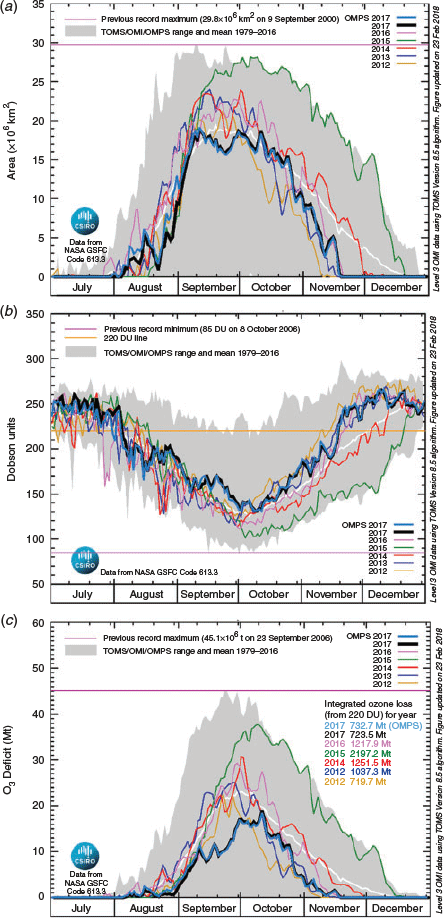
2 Ozone hole metrics
Table 1 contains the ranking for the 38 ozone holes adequately observed by satellite instruments since 1979 using eight metrics that measure the ‘size’ of the region where ozone is depleted (see the notes accompanying the table for the definition of each metric; metrics for 1995 and some metrics for 1994 are not included due to unavailability of the satellite data used).

|
As in previous reports of this series, Table 1 was produced using data processed with the version 8.5 algorithm from the Total Ozone Mapping Spectrometer (TOMS) series of satellite instruments, the Ozone Monitoring Instrument (OMI) on the Aura satellite and the Ozone Mapping Profiler Suite (OMPS) on the Suomi National Polar-orbiting Partnership satellite (see Klekociuk et al. 2014b and Krummel et al. 2019 for additional details). We use these specific measurements as they are made using a similar measurement technique. Similar metrics are produced by NASA (https://ozonewatch.gsfc.nasa.gov/, accessed 1 May 2020). TOMS measurements for part of 1994 and all of 1995 are not available, and consequently we have not evaluated some metrics in these years – other satellite measurements can potentially be used to fill the gap, but we have not applied those data here. There is a known drift in the TOMS measurements, particularly after 2000, which has been empirically corrected (Anton et al. 2010), and there are known differences between the overlapping TOMS and OMI measurements between 2004 and 2005 (McPeters et al. 2015; Kuttippurath et al. 2018). Additionally, there are differences in the spatial coverage of the individual instruments; for example, the field of view of the OMI instrument has been restricted due to an issue that arose in-orbit (McPeters et al. 2015). These calibration and field-of-view effects contribute to uncertainty and bias in our retrieved metrics. From comparison of metrics for 2005 produced separately from TOMS and OMI measurements, we find following relative differences: <2% for metrics 1, 2 and 5; <10% for metrics 3, 6 and 7; and ~20% for metric 4. These differences can be considered as notional upper limits of uncertainty in our metrics.
The first 7 metrics in Table 1 measure various aspects of the maximum area and depth of the ozone hole, and values for 2017 are highlighted in red font. The 2017 ozone hole ranked 29th in terms of maximum 15-day average area (metric 1); 28th in terms of daily maximum area (metric 2) and minimum 15-day averaged total column ozone (metric 3) and daily minimum total column ozone poleward of 35°S (metric 4) and daily minimum total column ozone averaged over the ozone hole (metric 5) and daily maximum ozone mass deficit (metric 6); and 26th in terms of the annual integrated ozone mass deficit (metric 7). The breakup date (metric 8; 18 November) was relatively early compared with other years, occurring ~2 weeks before the median date of other available years.
Years of similar overall ranking include 2002 (which featured an unprecedented stratospheric warming during September of that year), 1985 (which was early in the development of the Antarctic ozone hole phenomenon) and 2012 (during which the polar vortex exhibited large disturbances as discussed in Klekociuk et al. 2014b). Lower ranked ozone holes are generally those of the 1980s. Figure 1 shows time series of metrics 2, 4 and 6 over the latter half of each year from 2012 to 2017. Figure 1a indicates that the 2017 ozone hole began to develop at the start of August. During the first 2 weeks of August, the growth in area of the ozone hole was similar to the long-term climatology and generally ahead of the other years shown except for 2016. From ~15 to 25 August, and again from 10 to 25 September, two distinct episodes of significant disturbance to the polar vortex occurred – these episodes are discussed in Section 3. During both episodes, the area of the ozone hole was reduced compared with the long-term average at these times. From late September, the daily area metric started to decline in a manner that generally followed the long-term average up until the third week of October, after which the ozone hole rapidly decreased in area and ended in mid-November. The ozone hole breakdown date (metric 8) was similar to 2016, 2013, 2000 (a year of near-record ozone depletion) and 1991.
|
Figure 1c shows that the daily ozone mass deficit for 2017 was generally much lower than the long-term mean, particularly in the period up to mid-October. General reductions in the mass deficit coincided with the two periods of vortex disturbance noted above, whereas the daily minimum total column ozone was generally above the long-term mean during these periods (Fig. 1b).
The estimated total annual ozone mass deficit (metric 7) is shown in Fig. 2a, highlighting the relatively low value for 2017 in comparison with other years. Aside from years prior to and including 1986 which were early in the development of the ozone hole, lower ranked years for this metric are those in which the polar vortex was particularly disturbed in late-winter and spring: 2012 (Klekociuk et al. 2014b), 2002 (Newman and Nash 2005) and 1988 (Kreuger et al. 1989). Despite the level of variability from year-to-year, linear regression to the estimated annual equivalent effective stratospheric chlorine (EESC) level as shown in Fig. 2 explains 66% of the variance in the total annual ozone mass deficit. Tully et al. (2019b) examined trends of this metric, as well as metrics 1, 3 and ozone hole duration. After regressing against September 50-hPa mean temperature over 60–90°S, they found that the trend in the annual deficit over 2001–17 is −35.2 ± 27.4 (2σ) Mt year−1, which is significant at the 95% confidence limit. Tully et al. (2019b) also note that for all the metrics they considered, the behaviour of 2017 was within the 95% confidence limits of fitted trends over 2001–17 after allowance was made for interannual variability associated with Antarctic-region stratospheric temperatures.

|
The annual minimum total column ozone value obtained from daily measurements at Rothera, Antarctica, since 1996 (67.6°S and 68.1°W) is shown in Fig. 2b. As Rothera generally lies near the edge of the polar vortex in spring, the ozone column can be influenced by horizontal mixing at the vortex edge and zonal asymmetry of the circumpolar flow. As a result, the measurements may not necessarily reflect the general minimum value within the inner region of the vortex. However, it can be seen in the figure that 2017 showed a higher minimum value than most recent years, with larger values only in 2002 and 2010. This is generally consistent with the larger scale behaviour of minimum total column ozone across the ozone hole indicated by metrics 3 and 4 in Table 1.
3 Stratospheric dynamics and associated influences on the ozone hole
3.1 Stratospheric temperatures and winds
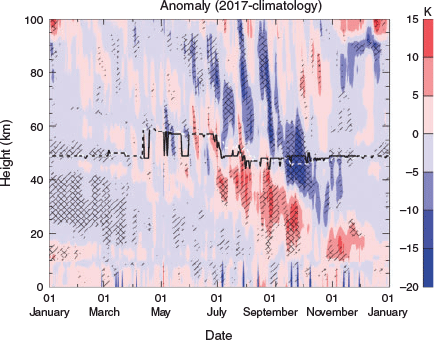
Figure 3 shows the time-height evolution of Antarctic-region air temperature anomalies during 2017 from measurements obtained by the microwave limb sounder (MLS) instrument on the Aura satellite. A region of generally below-average temperatures can be seen in the stratosphere for much of the period up until August. The upper border of this region gradually descended from the stratopause at the start of the year to be near 20 km in August.
|
Figure 3 shows that record low temperatures (over the climatological period since 2004) were apparent from January to March in the stratosphere and lowermost mesosphere (highlighted by the diagonal cross-hatching), whereas anomalously low stratospheric temperatures (below the climatological 10th percentile as shown by single hatching) occurred at times from May to July. Figure 3 indicates that during the first half of the year, warm anomalies above the stratopause appeared to generally descend into the stratosphere. The warm anomalies began to intensify near the stratopause from June and generally persisted in the lowermost stratosphere from August through November. Situated generally 20–30 km above the warmest stratospheric anomalies were descending cold anomalies that most noticeably appeared in the upper mesosphere during June, and which appeared to descend into in the upper stratosphere from early September to November.
Warm and cold anomalies descending into the stratosphere are apparent in other years of the MLS record (e.g. in 2012, a year of similar ozone hole metrics to 2017, as shown in fig. 13 of Klekociuk et al. 2014b). As discussed by Zhou et al. (2002) and Martineau and Son (2015) for the Arctic, the downward propagation of a large-scale warm anomaly from the upper stratosphere to the troposphere is seen in some years due to preconditioning of the stratosphere which allows upward forcing by planetary waves to lower the critical height for wave breaking over the course of the winter–spring season. This downward progression is also associated with the downward propagation through the stratosphere and troposphere of the negative mode of the North Atlantic Oscillation (which is the northern counterpart of the Southern Annular Mode (SAM)). In some years, the downward progression of the warm anomaly is blocked.
A further view of temperature anomalies in the troposphere and stratosphere with respect to a longer term climatology is provided in Fig. 4 as monthly average meridional cross sections for the period June to September from the ERA-Interim reanalysis (Dee et al. 2011). This figure also shows the monthly mean zonal winds and their climatological anomalies; the meridional gradient in the stratospheric winds provides an indication of the extent of the stratospheric polar vortex and the strength of the dynamical barrier formed by the westerly jet at its equatorward edge.

|
The temperature panels (left-hand column) of Fig. 4 for the polar latitudes (poleward of 60°S) show that cold stratospheric anomalies in June gave way to the descending warm anomaly noted in relation to Fig. 3 above from July. Throughout the period, the polar troposphere was generally anomalously cool, whereas the tropical and extratropical regions were anomalously warm.
For the zonal wind (middle and right-hand columns in Fig. 4), the westerlies near 60°S were anomalously strong in June throughout the stratosphere (and also between March and May (not shown)). The core of the polar stratospheric jet was noticeably shifted poleward in August and September as the upper regions of the vortex weakened (indicated by the anomalous negative zonal wind anomalies on the equatorward flank of the jet). In the upper tropical stratosphere, the winds became progressively more westerly as a descending shear developed in the phase of the QBO (which is discussed below). The zero wind line separating the tropical easterlies from the extratropical westerlies generally expanded poleward in the lower stratosphere from July. During the late summer and autumn months (February to May), the tropospheric westerlies were generally below-average strength (by typically 5 m s−1) equatorward of ~40°S (not shown). A region of below-average westerly flow in these months was also apparent in the troposphere and stratosphere poleward of ~60°S (excluding the region of tropospheric easterlies near the Antarctic coast) (not shown). From winter, the zone of weaker mid-latitude tropospheric winds persisted (except in July) and was situated ~10–20° further poleward (depending on height) in August and September. Throughout the tropical latitudes, the easterly flow was generally above average in strength from the beginning of the year, but consistent with the prevailing neutral phase of the El Niño–Southern Oscillation (http://www.cpc.ncep.noaa.gov/products/precip/CWlink/MJO/enso.shtml, accessed 1 May 2020).
Further information on the state of stratospheric temperatures, as well as the QBO and the tropospheric and stratosphere SAM indices is presented in Section A1.1 (Appendix 1) and Fig. A1.1. As noted in Section A1.1, the anomalously warm state of the lower stratosphere from July coincided with a shift of the QBO from a westerly phase to a more easterly phase (depending on height in the stratosphere), which would tend to favour greater disturbance of the stratospheric polar vortex by poleward-propagating planetary waves (Baldwin and Dunkerton 1998). The progressive shift in the stratospheric SAM index toward more negative values in winter and spring, which is apparent also for the tropospheric SAM at least through to October, was consistent with the findings of Zhou et al. (2002) and Martineau and Son (2015) for the effect of stratospheric preconditioning in the Arctic. The below-average polar tropospheric temperatures over the months shown in Fig. 4 were also consistent with the generally positive state of the tropospheric SAM index over the period.
3.2 Meridional heat transport
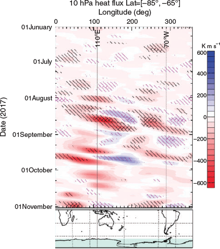
The poleward transport of heat provides an indicator of dynamical disturbances to the polar atmosphere produced by planetary waves originating in the troposphere at lower latitudes (Newman et al. 2001; Polvani and Waugh 2004). Figure 5 shows the evolution of eddy heat flux (evaluated as the product of the zonal anomalies in temperature and meridional wind speed) during 2017 from ERA-Interim reanalysis. In the 55–35°S latitude range (Fig. 5a), anomalously large poleward heat transport (negative heat flux values shown by filled red contours, indicating poleward and upward propagation of planetary waves) was apparent in the upper stratosphere (above 10 hPa) from early June, which became particularly intense during the middle and end of the month setting new extremes for the period since 1979 (as indicated by the cross-hatching in Fig. 5a during this period). In the polar cap region (Fig. 5b), anomalous poleward heat flux became apparent in mid-June in the upper stratosphere, with strong events that were significant at the 10th percentile penetrating to the tropopause (at ~100 hPa) and below ~21 August, 12 and 21 September, and 2 and 27 October (the dates of strongest poleward heat flux). Episodes of positive heat flux (blue filled contours, indicating downward and equatorward wave propagation) were also apparent at times, particularly in the upper mid-latitude stratosphere in early September.

|
Figure 6 shows the zonal distribution of heat flux at 10 hPa within the polar cap region from June to October inclusive. In general, two zonal bands containing the regions of strongest poleward heat transport (red filled contours) are apparent in this figure; a quasi-fixed band centred on ~70°W corresponding to the longitude of the southern tip of South America but extending at times ±90° or more in longitude, and a second band of similar width in the opposite hemisphere at longitudes to the west of Australia. In the second band, the poleward heat transport events tended to be more mobile in longitude over the course of the months shown. Overall, the longitudinal distribution showed a wave-2 zonal pattern, with the strongest events being centred in the eastern hemisphere. The most anomalous poleward heat transport feature in Fig. 6 centred near 170°E around 21 August was associated with the poleward displacement of the vortex by a stratospheric anticyclonic cell in the Australian sector discussed by Evtushevsky et al. (2019; their fig. 5). A second strong poleward transport feature on this date near 110°W (250°E) generally coincided with a region of reduced zonal wind speed at the equatorward edge of the polar vortex which was located above a negative geopotential height anomaly at 500 hPa that penetrated through to the 10 hPa level (shown in figure 5 of Evtushevsky et al. 2019). Additional regions of strong poleward heat transport can be seen at other times, particularly in September and October, which were associated with specific events noted above in relation to Fig. 5.
|
3.3 Stratospheric zonal asymmetries
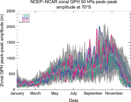
Disturbances that induce zonal asymmetry to the polar vortex are important in enhancing the mixing of air across the dynamical barrier at the equatorward edge of the vortex. This mixing can deplete the vortex of reactive reservoir species and bring in heat and replenish ozone, leading to an overall reduction in the size of the ozone hole (Solomon et al. 2014). The level of disturbance to the inner vortex in the lower stratosphere can be gauged by the examination of the range of geopotential height at high latitudes (Kravchenko et al. 2012; Evtushevsky et al. 2019), such as at 50 hPa and 70°S as shown in Fig. 7. Evtushevsky et al. (2019) have shown that the August average zonal temperature anomaly at this pressure level and latitude was anomalous in 1988, 2002 and 2017, and that the size of the anomaly for this month appears to have had a clear bearing on the overall size of the ozone hole in the following September to November period.
|
As discussed in relation to Fig. A1.2 in Section A1.2 of Appendix 1, the vortex near the 50-hPa level formed in early May and dissipated in mid-December. As can be seen by comparing Figs 6 and 7, large zonal variations in geopotential height accompanied the anomalous polar cap heat flux events noted in Section 3.2. The disturbances centred on 21 August, 12 September and 27 October were notable in setting new climatological extremes in the Antarctic lower stratosphere over the period since 1979. As discussed by Evtushevsky et al. (2019), the level of disturbance in the polar cap during August of 2017 was notable in comparison to the same month in 2002 and 1988.
Other notable polar cap disturbances in 2017 (as indicated by peaks in Fig. 7 lying above the climatological 90th percentile) occurred in late May, from mid- to late June (occurring ~the time of mid-latitude heat flux events noted above), mid-September (when parts of East Antarctica were situated outside the vortex, as discussed in relation to Figs A1.3 and A1.4 in Section A1.3 of Appendix 1), early October and from early to mid-November. The disturbances from late October caused the vortex to shift away from the pole and towards the African sector for a period of ~3 weeks, producing notably elevated levels of solar ultraviolet radiation at coastal sites in East Antarctica (see Section A1.4 and Fig. A1.5 of Appendix 1), and potentially enhancing photochemical deactivation of chlorine in the latter part of spring as inferred from enhanced chlorine nitrate total column abundances derived using Antarctic ground-based measurements (see Section A1.5 and Fig. A1.6 of Appendix 1).
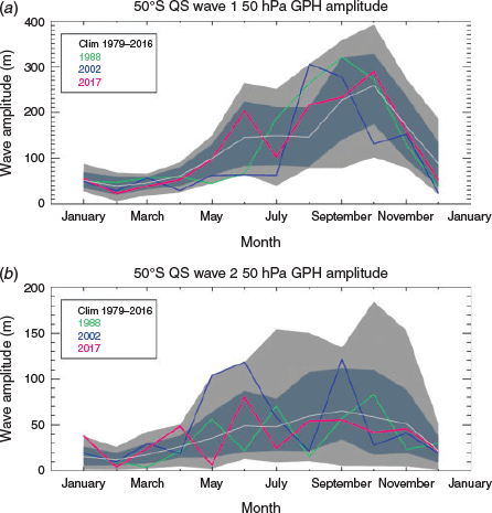
Quasi-stationary planetary waves, particularly with zonal wavenumber 1 (QSW-1), are a common feature in the Antarctic stratosphere from autumn to spring and strongly influence in the overall distribution of ozone both in the polar cap (Wirth 1993) and outside the vortex edge (McCormack et al. 1998). As shown in Fig. 8a, the amplitude of QSW-1 at 50° and 50 hPa for August in monthly average geopotential height was above the mean of the 1979–2016 climatology (5th largest observed and 1.2 standard deviations above the mean), and below the value for the notable years of 1988 and 2002. Similar enhanced QSW-1 activity in comparison with the climatology was also apparent between ~40 and ~65°S throughout the lower and middle stratosphere (not shown).
|
As can be seen in Fig. 8a, the QSW-1 amplitude was also above average in June; this month is also notable in showing enhanced zonal asymmetry in geopotential height in the polar cap (as shown in Fig. 5). The monthly average amplitude of quasi-stationary wave-2 (Fig. 8b) in 2017 was not generally notable; the wave amplitude was above average in June (as was also the case in 2002) but was near or slightly below average from July to October.
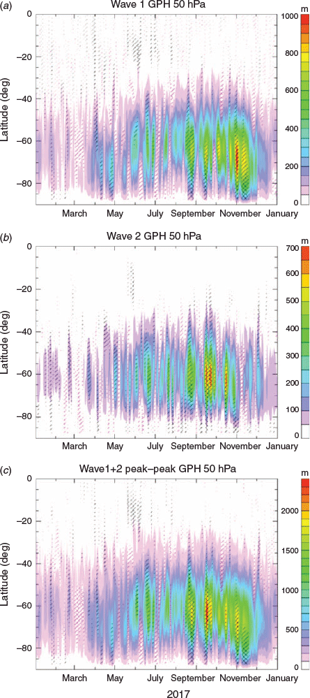
Figure 9 shows the daily zonal amplitudes of both wave 1 and 2 in 2017 for 50 hPa as a latitude-section. In this analysis, the wave amplitudes include components that may be either zonally stationary or travelling, although wave-1 is normally quasi-stationary. Anomalous wave-1 activity (indicated by single hatching in Fig. 9a) can be seen throughout the year, with climatological maximum values (indicated by cross-hatching) being reached poleward of 65°S in late August, early September and late October (corresponding to the climatological maxima discussed in relation to Fig. 7). Figure 9a also indicates that at low latitudes, wave-1 activity was also anomalous at times, particularly from April to June. Wave-2 (Fig. 9b), which generally extends to lower latitudes than wave-1, was generally enhanced at similar times to peaks in wave-1 activity.
|
The peak-to-peak amplitude of the sum of wave-1 and wave-2 (Fig. 9c) exhibited climatologically anomalous maxima at times in June, and from August to October, which corresponded to the periods of the strong poleward heat transport in the eastern longitude sector of the polar cap shown in Fig. 6. In geopotential height, the mean longitude of the maximum for QSW-1 at 50 hPa and 50°S varied from 158°E for August, 125°E for September 174°E for October (at 65°S, the wave maximum was ~10–30° further to the west in longitude), and it is apparent that the superposition of the quasi-stationary wave-1 and eastward travelling wave-2 was a key factor in enhancing poleward heat transport. Note that the poleward heat transport events shown in Fig. 6 generally show eastward progression with time, and this is consistent with the zonal motion of wave-2 which exhibited a period of ~10 days in GPH in the lower stratosphere at mid- and high latitudes (not shown).
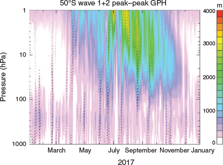
As can be seen in the time-height section of Fig. 10 for 50°S, anomalous superposition of waves 1 and 2 occurred simultaneously in the upper troposphere (pressures between ~250 and ~100 hPa) and the stratosphere in late March, and at times from June to September.
|
3.4 Planetary wave propagation
We now focus on the period June to September to examine the effects of and possible origins for the disturbances described in Section 3.3. Components of the Eliassen–Palm (EP) flux provide information on the zonal forcing by transient eddies (Edmon et al. 1980). Divergence of EP flux indicates deposition of westerly momentum into the zonal flow, upward EP flux is associated with poleward heat transport and upward wave propagation, and equatorward EP flux is associated with poleward meridional momentum flux. Figure 11 presents monthly mean latitude-height cross sections of EP flux divergence and scaled vertical and meridional components of EP flux for June to September 2017. In the upper row of panels in Fig. 11, regions of divergent (convergent) EP flux (negative (positive) contours in Fig. 11) indicate where eddies accelerated (decelerated) the westerly flow (on both the zonal average and monthly mean scales). The upper row of panels in Fig. 11 shows mixed patterns in the EP flux divergence in stratospheric polar region (poleward of 60°S). In all months, deceleration of the westerly flow (red contours) was apparent in the upper levels, particularly in September. In these months, there was also anomalous deceleration of the flow in regions of the mid-latitude stratosphere. In June and August, regions of anomalous acceleration of the flow (blue contours with magenta hatching) were apparent; in June, the acceleration was near the equatorward edge of the vortex in the lower stratosphere, whereas in August the acceleration was more towards the inner vortex. These regions of accelerated winds tally with strengthened westerlies in corresponding areas of Fig. 4.

|
The vertical and meridional components of EP flux are shown in the middle and bottom rows of panels in Fig. 11 respectively. In June there was anomalous poleward and upward EP flux in the troposphere at mid- and high-latitudes, whereas in the mid-latitude middle and upper stratosphere, the flux was anomalously directed equatorward and upward, generally overlapping with anomalous deceleration of the westerly flow. Overall, these features suggest the enhanced propagation of large-scale waves into the polar lower stratosphere from below, which dissipated in the upper stratosphere outside the vortex at midlatitudes causing weakening of the westerly flow.
In July, there was anomalous poleward and upward directed wave activity in the upper polar stratosphere, which appears associated with weakening of the flow in the upper vortex, and an associated warming (see the July temperature anomaly panel in Fig. 4). In August, anomalous upward and equatorward EP flux was apparent throughout the polar stratosphere; the cross-hatching in the meridional EP flux component for August indicated that poleward momentum forcing of the atmosphere was extreme over the climatological period in parts of the lower and upper stratosphere. The situation in September also showed generally enhanced poleward and upward wave propagation at high southern latitudes (similar to that in July), with strong deceleration of the upper vortex (which can also be seen in the zonal wind panels of Fig. 4).
3.5 Influence of the quasi-biennial oscillation on stratospheric composition
We now turn to the chemical composition of the polar vortex. Strahan et al. (2015) have shown that interannual variability of nitrous oxide (N2O) in the Antarctic stratospheric vortex in September is linked to the phase of the QBO ~1 year earlier. N2O is primarily released into the atmosphere at the surface and has a long atmospheric lifetime (~1 century) (Portmann et al. 2012) with no appreciable tropospheric sinks. In the stratosphere, ~10% of the N2O is converted to NO which destroys ozone in a catalytic cycle. Strahan et al. (2015) demonstrate that a negative (positive) N2O anomaly develops in the mid-latitude winter middle stratosphere during westerly (easterly) QBO phase which is consistent with the action of the descending QBO-induced vertical wind shear on the tropical overturning circulation. The QBO-induced N2O anomaly is subsequently transported into the Antarctic lower stratosphere and sets the chemical make-up of the polar vortex for the following winter. Strahan et al. (2015) and Strahan and Douglass (2017) have shown that the QBO also influences the interannual variability in the total amount of inorganic chlorine (Cly) available for ozone loss, with a general compact anticorrelation in the lower stratosphere between levels of Cly (adjusted for the annual decline rate in ozone depleting substances) and N2O (Schauffler et al. 2003; Strahan et al. 2014); increased Cly levels generally result in greater stratospheric ozone destruction.
Figure 12 shows mean N2O-mixing ratios and ozone-mixing ratio anomalies in the inner vortex for July, August and September of 2004–17 on two isentropic levels (450 and 600 K) in the lower stratosphere from Aura/MLS measurements. Figure 12a provides a similar analysis to that shown in figure 2 of Strahan and Douglass (2017). Three main features are apparent in Fig. 12a – (1) seemingly quasi-biennial interannual variability up to 2010, (2) a broad peak from 2010 to 2013 and (3) relatively consistent and low values for 2014–17. The behaviour at the higher isentropic level shown in Fig. 12b is somewhat different, showing relatively larger interannual variability, a transition from a high value in 2012 to a much lower value in 2013 (unlike the persistent high values in 2013 and 2014 on the 450 K surface), and a seemingly overall decline over the span of years analysed. Strahan and Douglass (2017), following on from Strahan et al. (2015), have ascribed the general peak in N2O values from 2010 to 2013 as due to the effects of the repeated winter easterly phase of the QBO over 2009–12. The winter QBO phase at 30 hPa was also westerly in 2003, 2005 and 2007 (https://www.cpc.ncep.noaa.gov/data/indices/qbo.u30.index, accessed 1 May 2020), and these years were also followed by peaks in the N2O mixing ratio as shown in Fig. 12a; this behaviour is also consistent with the expected QBO influence described by Strahan et al. (2015). In terms of the more recent years, the winters of 2013, 2015 and 2016 all had an easterly QBO phase (https://www.cpc.ncep.noaa.gov/data/indices/qbo.u30.index, accessed 13 May 2020); the QBO at 30 hPa became easterly in early 2014 but was in transition from westerly to easterly in the lower levels during the 2014 winter (https://iridl.ldeo.columbia.edu/maproom/Global/Atm_Circulation/QBO.html, accessed 1 May 2020). Newman et al. (2016) have discussed the persistence in the westerly QBO state from 2015 to 2016 in terms of anomalous northern tropical and subtropical forcing on the equatorial lower stratosphere from late 2015. Overall, the QBO influence on the N2O mixing ratio within the spring vortex described by Strahan et al. (2015) is consistent with there being reduced N2O in the vortex in 2014, 2016 and 2017, although the values observed generally appear much lower than for 2005, 2007 and 2009 (which, similar to 2014, 2016 and 2017, followed years in which the QBO was westerly during winter). The case of 2015 is less clear. For this year, the N2O mixing ratio on the 450 K surface would be expected to be higher than observed (as the QBO phase was easterly in the 2014 winter), and indeed the mixing ratio on the 600 K surface was higher than in 2014, 2016 and 2017. This suggests that the precise timing of the transition in the QBO phase as a function of height relative to winter in the preceding year may have been a factor.

|
Although the influence of the QBO on interannual variability of N2O in the vortex shown in Fig. 12a is generally consistent with the mechanism described by Strahan et al. (2015), the fraction of variance explained by correlation with standardised QBO indices is relatively low. For example, ~37% and 17% of the variance in the September values of respectively are explained by the linear correlation with the standardised QBO index at 30 hPa 1 year earlier.
The vortex-average ozone mixing ratios anomalies on both the 600 and 450 K isentropic surfaces are shown in Fig. 12c, d respectively. For 2017, the anomalies were generally near the mean over the observed years; in particular, the September values for the 450 K isentrope were similar to values over 2014–16. Strahan and Douglass (2017) in their figure 2 show for 2014–16 a small increase in the vortex-averaged Cly anomaly on the 450 K isentrope relative to 2010–13 which they attribute to the influence of the QBO. On the basis of the similarity of the vortex-averaged N2O mixing ratio on this isentrope in 2017 compared with 2014–16 shown in Fig. 12b, the anticorrelation between N2O and Cly in the vortex (Strahan et al. 2014) and accounting for the long-term downward trend in Cly levels (Strahan and Douglass 2017), it may be expected that Cly in the Antarctic vortex during 2017 was also elevated relative to 2010–13, and at least similar to 2016. The September N2O mixing ratio of Fig. 12b is significantly positively correlated with the corresponding ozone mixing ratio anomaly of Fig. 12d (r2 = 0.46), which also suggests that the westerly phase of the QBO in 2016 would have favoured increased ozone depletion in the lower stratosphere during the Antarctic spring of 2017. As the metrics for the ozone hole discussed in Section 2 indicate that total column ozone abundances over Antarctica were relatively high in 2017, we conclude that the influence of the 2016 QBO on the chemical make-up of the polar vortex in 2017 was not the strongest influence on the overall size of the 2017 ozone hole.
4 Summary and conclusions
We have examined meteorological conditions and ozone concentrations in the Antarctic atmosphere during 2017 using a variety of data sources, including meteorological assimilations, satellite remote sensing measurements and ground-based instruments and ozonesondes.
The overall severity of ozone loss during the 2017 Antarctic ozone hole was notably low in comparison with other years on record. In terms of maximum 15-day average area, the 2017 ozone hole was ranked 29th in the available 38 years of records since 1979 (which excludes 1995). The maximum 15-day average area was ~60% of the largest value for this metric which was observed in 2000. The 2017 ozone hole was ranked 26th in terms of the estimated total ozone mass deficit and produced ~29% of the deficit observed in 2000.
The overall level of the ozone metrics was consistent with there being reduced efficiency of chemical depletion within the polar vortex due to relatively high levels of meteorological variability. The upper levels of the vortex became most noticeably disturbed by planetary waves from June, and the disturbances penetrated into the lower stratosphere from August. Warming of the vortex and mixing of air across the vortex barrier (as indicated by episodic reduction in the area enclosed by contours of potential vorticity) were pronounced during August and September, which significantly impeded the normal development of the ozone hole.
The below-average speed of the mid-latitude tropospheric westerly winds in August and September potentially aided the development of strong disturbances to the vortex in these months. By the Charney–Drazin theorem (Charney and Drazin 1961), vertical propagation of low-order planetary waves is permitted only when the background flow is westerly and below a critical threshold. The region of reduced tropospheric wind speed in August and September was generally at the latitudes where the EP flux indicates poleward and upward wave propagation, and where the amplitude of QSW-1 in the lower stratosphere peaks (see figure 2 of Evtushevsky et al. 2019). The generally above-average QSW-1 amplitudes in winter and spring (and particularly in August) in the lower stratosphere shown in Fig. 8 were thus possibly influenced by the lowering of the critical wave propagation threshold as a result of the weaker tropospheric westerlies, and potentially also by the generally weakening of the stratospheric mid-latitude westerlies that also took place in August in September as shown in Fig. 4.
Evtushevsky et al. (2019) highlight the potential role of mid-latitude stratospheric anticyclones in helping destabilise and erode the polar vortex in 2017. These anticyclones are a feature of the Southern Hemisphere stratospheric circulation in winter and spring (Harvey et al. 2002) as the polar vortex starts to weaken and generally appear in the South American, African and Australian sectors. Generally one or two anticyclones are apparent at any particular time and may travel east or west. The indication from Fig. 11 of anomalous equatorward and poleward wave propagation (and increased poleward momentum flux and deceleration of the westerly winds) in the stratospheric mid-latitudes supports there being an intensification of stratospheric mid-latitude anticyclonic activity in August and September. On the equatorward side of the anticyclones, the flow tends to oppose and weaken the prevailing westerlies, whereas on the poleward side of the anticyclones, the westerly flow at the edge of the vortex tends to be reinforced, which would produce patterns of stratospheric zonal wind anomalies at these latitudes similar to those in Fig. 4. Additionally, the movement of the zero zonal wind critical line apparent in Fig. 4, due to the strengthening of the easterly QBO phase in the lower tropical stratosphere noted in Section 5.1, by the Holton–Tan effect would be expected to focus planetary wave activity at mid- and low latitudes (Holton and Tan 1980). The resulting poleward momentum forcing through the intensification of the stratospheric anticyclones has been shown to distort the polar vortex, displacing its boundary to lower latitudes where erosion by geostrophic adjustment would be more likely (Harvey et al. 2002).
An additional factor that appears important for the development of the mid-latitude stratospheric anticyclones was the downward propagation of the warm anomalies from the upper stratosphere through to the troposphere over the course of the winter and spring. As discussed by Zhou et al. (2002), this feature is consistent with the lowering of the critical height for planetary wave breaking by upward propagation of wave activity. The expected downward weakening of the zonal winds is consistent with the observed patterns in Fig. 4 and may have acted separately to, or in concert with, the Holton–Tan effect discussed above to intensify the stratospheric anticyclones. The ability for planetary waves to penetrate through the stratosphere and precondition the upper levels appears to have been favoured at high latitudes during the preceding late summer and autumn by below-average zonal winds in the troposphere and lower stratosphere, which may have been aided in the troposphere by the prevailing negative phase of the SAM in this period.
Of further note regarding the above-average amplitude of QSW-1 in the winter and spring stratosphere is the possible role of this feature in enhancing disturbance of the vortex in spring. As discussed by Evtushevsky et al. (2019), QSW-1 having a large amplitude in the polar stratosphere does not necessarily in itself weaken the vortex and mitigate ozone depletion. However, the possibility of QSW-1 helping to amplify the overall effect of travelling wave-1 and wave-2 disturbances is potentially an important factor in the strong asymmetry exhibited by the polar vortex in August and September 2017. This view is supported by the timing of the enhanced sum of the wave-1 and wave-2 contributions shown in Fig. 9 with the anomalous poleward heat transport events shown in Fig. 6, and the preference for the strongest poleward heat transport to occur where the location of the Australian anticyclone generally coincided with the maximum geopotential height anomaly of QSW-1 as discussed in Section 3.3.
Based on consideration of observed levels of nitrous oxide in the polar vortex, the westerly phase of the QBO in 2016 likely favoured the levels of stratospheric inorganic chlorine over Antarctica during the spring of 2017 that were similar to those during 2016 when the ozone hole was relatively larger. However, the overall level of erosion of the polar vortex in August and September by dynamical variability significantly impeded the development of the ozone hole, and this was the main factor that dictated the overall level of ozone loss in 2017.
Acknowledgements
We acknowledge the Department of Environment and Energy of the Australian Government for support of this work, and the assistance of the following people: Jeff Ayton and the AAD’s Antarctic Medical Practitioners in collecting the solar UV data, BoM staff/observers in collecting surface and upper air measurements at Cape Grim, Macquarie Island and Davis, and Antarctica New Zealand expeditioners in collecting measurements at Arrival Heights. Measurements at Arrival Heights are core-funded by NIWA through New Zealand’s Ministry of Business, Innovation and Employment. The TOMS, OMI and OMPS data used in this study are provided by the NASA Goddard Space Flight Center, Atmospheric Chemistry & Dynamics Branch, Code 613.3. Aura/MLS data used in this study were acquired as part of the NASA’s Earth–Sun System Division and archived and distributed by the Goddard Earth Sciences (GES) Data and Information Services Center (DISC) Distributed Active Archive Center (DAAC). UKMO reanalysis data were obtained from the British Atmospheric Data Centre (http://badc.nerc.ac.uk, accessed 1 May 2020). NCEP–NCAR reanalysis data were obtained from the National Oceanic and Atmospheric Administration Earth System Research laboratory, Physical Sciences Division. ERA-Interim reanalysis data were obtained from the data portal of the European Centre for Medium-Range Weather Forecasts (https://apps.ecmwf.int/datasets/, accessed 1 May 2020). Davis ozonesonde measurements are available from the World Ozone and Ultraviolet Radiation Data Centre (https://woudc.org, accessed 1 May 2020). Part of this work was performed under Project 4293 of the Australian Antarctic Science program. This research did not receive any specific grant funding.
References
Anton, M., Vilaplana, J. M., Kroon, M., Serrano, A., Parias, M., Cancillo, M. L., and de la Morena, B. A. (2010). The empirically corrected EP-TOMS total ozone data against Brewer measurements at El Arenosillo (southwestern Spain). IEEE Trans. Geosci. Remote Sens. 48, 3039–3045.| The empirically corrected EP-TOMS total ozone data against Brewer measurements at El Arenosillo (southwestern Spain).Crossref | GoogleScholarGoogle Scholar |
Baldwin, M. P., and Dunkerton, T. J. (1998). Quasi-biennial modulations of the Southern Hemisphere stratospheric polar vortex. Geophys. Res. Lett. 25, 3343–3346.
| Quasi-biennial modulations of the Southern Hemisphere stratospheric polar vortex.Crossref | GoogleScholarGoogle Scholar |
Baldwin, M. P., and Dunkerton, T. J. (2001). Stratospheric harbingers of anomalous weather regimes. Science 294, 581–584.
| Stratospheric harbingers of anomalous weather regimes.Crossref | GoogleScholarGoogle Scholar |
Charney, J. G., and Drazin, P. G. (1961). Propagation of planetary-scale disturbances from the lower into the upper atmosphere. J. Geophys. Res. 66, 83–109.
| Propagation of planetary-scale disturbances from the lower into the upper atmosphere.Crossref | GoogleScholarGoogle Scholar |
Chipperfield, M. P., Bekki, S., Dhomse, S., Harris, N. R. P., Hassler, B., Hossaini, R., Steinbrecht, W., Thiéblemont, R., and Weber, M. (2017). Detecting recovery of the stratospheric ozone layer. Nature 549, 211–218.
| Detecting recovery of the stratospheric ozone layer.Crossref | GoogleScholarGoogle Scholar |
Dee, D. P., Uppala, S. M., Simmons, A. J., Berrisford, P., Poli, P., Kobayashi, S., Andrae, U., Balmaseda, M. A., Balsamo, G., Bauer, P., Bechtold, P., Beljaars, A. C. M., van de Berg, L., Bidlot, J., Bormann, N., Delsol, C., Dragani, R., Fuentes, M., Geer, A. J., Haimberger, L., Healy, S. B., Hersbach, H., Hólm, E. V., Isaksen, L., Kållberg, P., Köhler, M., Matricardi, M., McNally, A. P., Monge-Sanz, B. M., Morcrette, J.-J., Park, B.-K., Peubey, C., de Rosnay, P., Tavolato, C., Thépaut, J.-N., and Vitart, F. (2011). The ERA-Interim reanalysis: configuration and performance of the data assimilation system. Q. J. R. Meteorol. Soc. 137, 553–597.
| The ERA-Interim reanalysis: configuration and performance of the data assimilation system.Crossref | GoogleScholarGoogle Scholar |
Edmon, H. J., Hoskins, B. J., and McIntyre, M. E. (1980). Eliassen-Palm cross sections for the troposphere. J. Atmos. Sci. 37, 2600–2616.
| Eliassen-Palm cross sections for the troposphere.Crossref | GoogleScholarGoogle Scholar |
Evtushevsky, O. M., Klekociuk, A. R., Kravchenko, V. O., Milinevsky, G. P., and Grytsai, A. V. (2019). The influence of large amplitude planetary waves on the Antarctic ozone hole of austral spring 2017. J. South. Hemisph. Earth Syst. Sci. 69, 57–64.
| The influence of large amplitude planetary waves on the Antarctic ozone hole of austral spring 2017.Crossref | GoogleScholarGoogle Scholar |
Fortuin, J. P. F., and Kelder, H. (1998). An ozone climatology based on ozonesonde and satellite measurements. J. Geophys. Res. 103, 31709–31734.
| An ozone climatology based on ozonesonde and satellite measurements.Crossref | GoogleScholarGoogle Scholar |
Fraser, P., Krummel, P., Steele, P., Trudinger, C., Etheridge, D., Derek, D., O’Doherty, S., Simmonds, P., Miller, B., Muhle, J., Weiss, R., Oram, D., Prinn, R., and Wang R. (2014). Equivalent effective stratospheric chlorine from Cape Grim Air Archive, Antarctic firn and AGAGE global measurements of ozone depleting substances. In ‘Baseline Atmospheric Program (Australia) 2009–2010’. (Eds N. Derek, P. Krummel, and S. Cleland) pp. 17–23. (Australian Bureau of Meteorology and CSIRO Marine and Atmospheric Research: Melbourne, Vic., Australia.)
Harvey, V. L., Pierce, R. B., and Hitchman, M. H. (2002). A climatology of stratospheric polar vortices and anticyclones. J. Geophys. Res. 107, 4442.
| A climatology of stratospheric polar vortices and anticyclones.Crossref | GoogleScholarGoogle Scholar |
Holton, J. R., and Tan, H.-C. (1980). The influence of the equatorial quasi-biennial oscillation on the global circulation at 50 mb. J. Atmos. Sci. 37, 2200–2208.
| The influence of the equatorial quasi-biennial oscillation on the global circulation at 50 mb.Crossref | GoogleScholarGoogle Scholar |
Huck, P. E., McDonald, A. J., Bodeker, G. E., and Struthers, H. (2005). Interannual variability in Antarctic ozone depletion controlled by planetary waves and polar temperature. Geophys. Res. Lett. 32, L13819.
| Interannual variability in Antarctic ozone depletion controlled by planetary waves and polar temperature.Crossref | GoogleScholarGoogle Scholar |
Kalnay, E., Kanamitsu, M., Kistler, R., Collins, W., Deaven, D., Gandin, L., Iredell, M., Saha, S., White, G., Woollen, J., Zhu, Y., Leetmaa, A., Reynolds, R., Chelliah, M., Ebisuzaki, W., Higgins, W., Janowiak, J., Mo, K. C., Ropelewski, C., Wang, J., Jenne, R., and Joseph, D. (1996). The NCEP/NCAR 40-Year Reanalysis Project. Bull. Am. Meteor. Soc. 77, 437–471.
| The NCEP/NCAR 40-Year Reanalysis Project.Crossref | GoogleScholarGoogle Scholar |
Klekociuk, A. R., Tully, M. B., Alexander, S. P., Dargaville, R. J., Deschamps, L. L., Fraser, P. J., Gies, H. P., Henderson, S. I., Javorniczky, J., Krummel, P. B., Petelina, S. V., Shanklin, J. D., Siddaway, J. M., and Stone, K. A. (2011). The Antarctic ozone hole during 2010. Aust. Met. Oceanog. J. 61, 253–267.
| The Antarctic ozone hole during 2010.Crossref | GoogleScholarGoogle Scholar |
Klekociuk, A. R., Tully, M. B., Krummel, P. B., Gies, H. P., Petelina, S. V., Alexander, S. P., Deschamps, L. L., Fraser, P. J., Henderson, S. I., Javorniczky, J., Shanklin, J. D., Siddaway, J. M., and Stone, K. A. (2014a). The Antarctic ozone hole during 2011. Aust. Met. Oceanog. J. 64, 293––311.
| The Antarctic ozone hole during 2011.Crossref | GoogleScholarGoogle Scholar |
Klekociuk, A. R., Tully, M. B., Krummel, P. B., Gies, H. P., Alexander, S. P., Fraser, P. J., Henderson, S. I., Javorniczky, J., Petelina, S. V., Shanklin, J. D., Schofield, R., and Stone, K. A. (2014b). The Antarctic ozone hole during 2012. Aust. Met. Oceanog. J. 64, 313–330.
| The Antarctic ozone hole during 2012.Crossref | GoogleScholarGoogle Scholar |
Klekociuk, A. R., Tully, M. B., Krummel, P. B., Gies, H. P., Alexander, S. P., Fraser, P. J., Henderson, S. I., Javorniczky, J., Shanklin, J. D., Schofield, R., and Stone, K. A. (2015). The Antarctic ozone hole during 2013. Aust. Met. Oceanog. J. 65, 247–266.
| The Antarctic ozone hole during 2013.Crossref | GoogleScholarGoogle Scholar |
Kohlhepp, R., Ruhnke, R., Chipperfield, M. P., De Mazière, M., Notholt, J., Barthlott, S., Batchelor, R. L., Blatherwick, R. D., Blumenstock, Th., Coffey, M. T., Demoulin, P., Fast, H., Feng, W., Goldman, A., Griffith, D. W. T., Hamann, K., Hannigan, J. W., Hase, F., Jones, N. B., Kagawa, A., Kaiser, I., Kasai, Y., Kirner, O., Kouker, W., Lindenmaier, R., Mahieu, E., Mittermeier, R. L., Monge-Sanz, B., Morino, I., Murata, I., Nakajima, H., Palm, M., Paton-Walsh, C., Raffalski, U., Reddmann, Th., Rettinger, M., Rinsland, C. P., Rozanov, E., Schneider, M., Senten, C., Servais, C., Sinnhuber, B.-M., Smale, D., Strong, K., Sussmann, R., Taylor, J. R., Vanhaelewyn, G., Warneke, T., Whaley, C., Wiehle, M., and Wood, S. W. (2012). Observed and simulated time evolution of HCl, ClONO2, and HF total column abundances. Atmos. Chem. Phys. 12, 3527–3556.
| Observed and simulated time evolution of HCl, ClONO2, and HF total column abundances.Crossref | GoogleScholarGoogle Scholar |
Kreuger, A. J., Stolarski, R. S., and Schoeberl, M. R. (1989). Formation of the 1988 Antarctic ozone hole. Geophys. Res. Lett. 16, 381–384.
| Formation of the 1988 Antarctic ozone hole.Crossref | GoogleScholarGoogle Scholar |
Kravchenko, V. O., Evtushevsky, O. M., Grytsai, A. V., Klekociuk, A. R., Milinevsky, G. P., and Grytsai, Z. I. (2012). Quasi-stationary planetary waves in late winter Antarctic stratosphere temperature as a possible indicator of spring total ozone. Atmos. Chem. Phys. 12, 2865–2879.
| Quasi-stationary planetary waves in late winter Antarctic stratosphere temperature as a possible indicator of spring total ozone.Crossref | GoogleScholarGoogle Scholar |
Krummel, P. B., Klekociuk, A. R., Tully, M. B., Gies, H. P., Alexander, S. P., Fraser, P. J., Henderson, S. I., Schofield, R., Shanklin, J. D., and Stone, K. A. (2019). The Antarctic ozone hole during 2014. J. South. Hemisph. Earth Syst. Sci. 69, 1–15.
| The Antarctic ozone hole during 2014.Crossref | GoogleScholarGoogle Scholar |
Kurzeja, R. J. (1984). Spatial variability of total ozone at high latitudes in winter. J. Atmos. Sci. 41, 695–697.
| Spatial variability of total ozone at high latitudes in winter.Crossref | GoogleScholarGoogle Scholar |
Kuttippurath, J., Kumar, P., Nair, P. J., and Chakraborty, A. (2018). Accuracy of satellite total column ozone measurements in polar vortex conditions: Comparison with ground-based observations in 1979–2013. Remote Sens. Environ. 209, 648–659.
| Accuracy of satellite total column ozone measurements in polar vortex conditions: Comparison with ground-based observations in 1979–2013.Crossref | GoogleScholarGoogle Scholar |
McCormack, J. P., Miller, A. J., and Nagatini, R. (1998). Interannual variability in the spatial distribution of extratropical total ozone. Geophys. Res. Lett. 25, 2153–2156.
| Interannual variability in the spatial distribution of extratropical total ozone.Crossref | GoogleScholarGoogle Scholar |
McPeters, R. D., Labow, G. J., and Johnson, B. J. (1997). A satellite-derived ozone climatology for balloonsonde estimation of total column ozone. J. Geophys. Res. 102, 8875–8885.
| A satellite-derived ozone climatology for balloonsonde estimation of total column ozone.Crossref | GoogleScholarGoogle Scholar |
McPeters, R. D., Frith, S., and Labow, G. J. (2015). OMI total column ozone: extending the long-term data record. Atmos. Meas. Tech. 8, 4845–4850.
| OMI total column ozone: extending the long-term data record.Crossref | GoogleScholarGoogle Scholar |
Manney, G. L., Daffer, W. H., Zawodny, J. M., Bernath, P. F., Hoppel, K. W., Walker, K. A., Knosp, B. W., Boone, C., Remsberg, E. E., Santee, M. L., Harvey, V. L., Pawson, S., Jackson, D. R., Deaver, L., McElroy, C. T., McLinden, C. A., Drummond, J. R., Pumphrey, H. C., Lambert, A., Schwartz, M. J., Froidevaux, L., McLeod, S., Takacs, L. L., Suarez, , Max, J., Trepte, C. R., Cuddy, , David, C., Livesey, N. J., Harwood, R. S., and Waters, J. W. (2007). Solar occultation satellite data and derived meteorological products: sampling issues and comparisons with Aura Microwave Limb Sounder. J. Geophys. Res. 112, D24S50.
| Solar occultation satellite data and derived meteorological products: sampling issues and comparisons with Aura Microwave Limb Sounder.Crossref | GoogleScholarGoogle Scholar |
Marshall, G. J. (2003). Trends in the Southern Annular Mode from observations and reanalyses. J. Clim. 16, 4134–4143.
| Trends in the Southern Annular Mode from observations and reanalyses.Crossref | GoogleScholarGoogle Scholar |
Martineau, P., and Son, S.-W. (2015). Onset of circulation anomalies during stratospheric vortex weakening events: the role of planetary-scale waves. J. Clim. 28, 7347–7370.
| Onset of circulation anomalies during stratospheric vortex weakening events: the role of planetary-scale waves.Crossref | GoogleScholarGoogle Scholar |
Nash, E. R., Newman, P. A., Rosenfield, J. E., and Schoeberl, M. R. (1996). An objective determination of the polar vortex using Ertel’s potential vorticity. J. Geophys. Res. 101, 9471–9478.
| An objective determination of the polar vortex using Ertel’s potential vorticity.Crossref | GoogleScholarGoogle Scholar |
Newman, P. A., Nash, E. R., and Rosenfield, J. E. (2001). What controls the temperature in the Arctic stratosphere in the spring? J. Geophys. Res. 106, 19999–20010.
| What controls the temperature in the Arctic stratosphere in the spring?Crossref | GoogleScholarGoogle Scholar |
Newman, P. A., and Nash, E. R. (2005). The unusual Southern Hemisphere stratosphere winter of 2002. J. Atmos. Sci. 62, 614–628.
| The unusual Southern Hemisphere stratosphere winter of 2002.Crossref | GoogleScholarGoogle Scholar |
Newman, P. A., Kawa, S. R., and Nash, E. R. (2004). On the size of the Antarctic ozone hole. Geophys. Res. Lett. 31, L21104.
| On the size of the Antarctic ozone hole.Crossref | GoogleScholarGoogle Scholar |
Newman, P. A., Coy, L., Pawson, S., and Lait, L. R. (2016). The anomalous change in the QBO in 2015–2016. Geophys. Res. Lett. 43, 8791–8797.
| The anomalous change in the QBO in 2015–2016.Crossref | GoogleScholarGoogle Scholar |
Poli, P., Healy, S. B., and Dee, D. P. (2010). Assimilation of Global Positioning System radio occultation data in the ECMWF ERA–Interim reanalysis. Q. J. R. Meteorol. Soc. 136, 1972–1990.
| Assimilation of Global Positioning System radio occultation data in the ECMWF ERA–Interim reanalysis.Crossref | GoogleScholarGoogle Scholar |
Polvani, L. M., and Waugh, D. W. (2004). Upward wave activity flux as a precursor to extreme stratospheric events and subsequent anomalous surface weather regimes. J. Clim. 17, 3548–3554.
| Upward wave activity flux as a precursor to extreme stratospheric events and subsequent anomalous surface weather regimes.Crossref | GoogleScholarGoogle Scholar |
Portmann, R. W., Daniel, J. S., and Ravishankara, A. R. (2012). Stratospheric ozone depletion due to nitrous oxide: influences of other gases. Philos. Trans. R. Soc. B: Biol. Sci. 367, 1256–1264.
| Stratospheric ozone depletion due to nitrous oxide: influences of other gases.Crossref | GoogleScholarGoogle Scholar |
Roscoe, H. K., Johnston, P. V ., Van Roozendael, M., Richter, A., Preston, K., Lambert, J. C., Hermans, C., de Kuyper, W., Dzenius, S., Winterath, T., Burrows, J., Sarkissian, A., Goutail, F., Pommereau, J. P., d’Almeida, E., Hottier, J., Coureul, C., Ramond, D., Pundt, I., Bartlet, L. M., Kerr, J. E., Elokhov, A., Giovanelli, G., Ravegnani, F., Premudan, M., Kostadinov, M., Erle, F., Wagner, T., Pfeilsticker, K., Kenntner, M., Marquand, L. C., Gil, M., Puentedura, O., Arlander, W., Kaastad-Hoiskar, B. A., Tellefsen, C. W., Heese, C. W., Jones, R. L., Aliwell, S. R., and Freshwater, R. A. (1999). Slant column measurements of O3 and NO2 during the NDSC intercomparison of zenith-sky UV visible spectrometers in June 1996. J. Atmos. Chem. 32, 281–314.
| Slant column measurements of O3 and NO2 during the NDSC intercomparison of zenith-sky UV visible spectrometers in June 1996.Crossref | GoogleScholarGoogle Scholar |
Schauffler, S. M., Atlas, E. L., Donnelly, S. G., Andrews, A., Montzka, S. A., Elkins, J. W., Hurst, D. F., Romashkin, P. A., Dutton, G. S., and Stroud, V. (2003). Chlorine budget and partitioning during the Stratospheric Aerosol and Gas Experiment (SAGE) III Ozone Loss and Validation Experiment (SOLVE). J. Geophys. Res. 108, 4173.
| Chlorine budget and partitioning during the Stratospheric Aerosol and Gas Experiment (SAGE) III Ozone Loss and Validation Experiment (SOLVE).Crossref | GoogleScholarGoogle Scholar |
Schoeberl, M. R., Douglass, A. R., Kawa, S. R., Dessler, A. E., Newman, P. A., Stolarski, R. S., Roche, A. E., Waters, J. W., and Russell, J. M. (1996). Development of the Antarctic ozone hole. J. Geophys. Res.: Atmos. 101, 20909–20924.
| Development of the Antarctic ozone hole.Crossref | GoogleScholarGoogle Scholar |
Schwartz, M. J., Lambert, A., Manney, G. L., Read, W. G., Livesey, N. J., Froidevaux, L., Ao, C. O., Bernath, P. F., Boone, C. D., Cofield, R. E., Daffer, W. H., Drouin, B. J., Fetzer, E. J., Fuller, R. A., Jarnot, R. F., Jiang, J. H., Jiang, Y. B., Knosp, B. W., Krüger, K. R., Li, J.-L. F., Mlynczak, M. G., Pawson, S., Russell, J. M., Santee, M. L., Snyder, W. V., Stek, P. C., Thurstans, R. P., Tompkins, A. M., Wagner, P. A., Walker, K. A., Waters, J. W., and Wu, D. L. (2008). Validation of the Aura Microwave Limb Sounder temperature and geopotential height measurements. J. Geophys. Res. 113, D15S11.
| Validation of the Aura Microwave Limb Sounder temperature and geopotential height measurements.Crossref | GoogleScholarGoogle Scholar |
Solomon, S., Haskins, J., Ivy, D. J., and Min, F. (2014). Fundamental differences between Arctic and Antarctic ozone depletion. Proc. Natl. Acad. Sci. U.S.A. 111, 6220–6225.
| Fundamental differences between Arctic and Antarctic ozone depletion.Crossref | GoogleScholarGoogle Scholar |
Solomon, S., Ivy, D. J., Kinnison, D., Mills, M. J., Neely, R. R., and Schmidt, A. (2016). Emergence of healing in the Antarctic ozone layer. Science 353, 269–274.
| Emergence of healing in the Antarctic ozone layer.Crossref | GoogleScholarGoogle Scholar |
Strahan, S. E., Douglass, A. R., Newman, P. A., and Steenrod, S. D. (2014). Inorganic chlorine variability in the Antarctic vortex and implications for ozone recovery. J. Geophys. Res. Atmos. 119, 14098–14109.
| Inorganic chlorine variability in the Antarctic vortex and implications for ozone recovery.Crossref | GoogleScholarGoogle Scholar |
Strahan, S. E., Oman, L. D., Douglass, A. R., and Coy, L. (2015). Modulation of Antarctic vortex composition by the quasi-biennial oscillation. Geophys. Res. Lett. 42, 4216–4223.
| Modulation of Antarctic vortex composition by the quasi-biennial oscillation.Crossref | GoogleScholarGoogle Scholar |
Strahan, S. E., and Douglass, A. R. (2017). Decline in Antarctic ozone depletion and lower stratospheric chlorine determined from Aura Microwave Limb Sounder observations. Geophys. Res. Lett. 44, .
| Decline in Antarctic ozone depletion and lower stratospheric chlorine determined from Aura Microwave Limb Sounder observations.Crossref | GoogleScholarGoogle Scholar |
Swinbank, R., and O’Neill, A. A. (1994). Stratosphere-troposphere data assimilation system. Mon. Wea. Rev. 122, 686–702.
| Stratosphere-troposphere data assimilation system.Crossref | GoogleScholarGoogle Scholar |
Tully, M. B., Klekociuk, A. R., Deschamps, L. L., Henderson, S. I., Krummel, P. B., Fraser, P. J., Shanklin, J. D., Downey, A. H., Gies, H. P., and Javorniczky, J. (2008). The 2007 Antarctic ozone hole. Aust. Met. Mag. 57, 279–298.
Tully, M. B., Klekociuk, A. R., Alexander, S. P., Dargaville, R. J., Deschamps, L. L., Fraser, P. J., Gies, H. P., Henderson, S. I., Javorniczky, J., Krummel, P. B., Petelina, S. V., Shanklin, J. D., Siddaway, J. M., and Stone, K. A. (2011). The Antarctic ozone hole during 2008 and 2009. Aust. Met. Oceanog. J. 61, 77–90.
| The Antarctic ozone hole during 2008 and 2009.Crossref | GoogleScholarGoogle Scholar |
Tully, M. B., Klekociuk, A. R., Krummel, P. B., Gies, H. P., Alexander, S. P., Fraser, P. J., Henderson, S. I., Schofield, R., Shanklin, J. D., and Stone, K. A. (2019a). The Antarctic ozone hole during 2015 and 2016. J. South. Hemisph. Earth Syst. Sci. 69, 16–28.
| The Antarctic ozone hole during 2015 and 2016.Crossref | GoogleScholarGoogle Scholar |
Tully, M. B., Krummel, P. B., and Klekociuk, A. R. (2019b). Trends in Antarctic ozone hole metrics 2001–17. J. South. Hemisph. Earth Syst. Sci. 69, 52–56.
| Trends in Antarctic ozone hole metrics 2001–17.Crossref | GoogleScholarGoogle Scholar |
Watson, P. A. G., and Gray, L. G. (2014). How does the quasi-biennial oscillation affect the stratospheric polar vortex? J. Atmos. Sci. 71, 391–409.
| How does the quasi-biennial oscillation affect the stratospheric polar vortex?Crossref | GoogleScholarGoogle Scholar |
WHO (World Health Organization) (2002). Global Solar UV Index: A Practical Guide. (WHO (World Health Organization): Geneva.)
Wirth, V. (1993). Quasi-stationary planetary waves in total ozone and their correlation with lower stratospheric temperature. J. Geophys. Res. 98, 8873–8882.
| Quasi-stationary planetary waves in total ozone and their correlation with lower stratospheric temperature.Crossref | GoogleScholarGoogle Scholar |
Zhou, S., Miller, A. J., Wang, J., and Angell, J. K. (2002). Downward propagating temperature anomalies in the preconditioned polar stratosphere. J. Clim. 15, 781–792.
| Downward propagating temperature anomalies in the preconditioned polar stratosphere.Crossref | GoogleScholarGoogle Scholar |
A1.1 Polar atmospheric indices
Figure A1.1a shows monthly mean temperature anomalies over the Antarctic region during 2017 from the ERA-Interim reanalysis at pressure levels of (top to bottom) 10 (~30 km altitude), 50 (~18 km altitude) and 100 hPa (~12 km altitude). At all three levels, temperatures in 2017 were below the climatological average up to and including July, with most months at 10 and 50 hPa being below or near the 10th percentile for the preceding decade (indicated by ranks 9 or 10). Positive temperature anomalies occurred at all three levels from August to October. In November and December, above-average polar cap temperatures occurred in both months at 100 and 50 hPa, whereas temperatures at 10 hPa were below average in both months.

|
The NCEP standardised 30-hPa quasi-biennial oscillation (QBO) index (https://www.cpc.ncep.noaa.gov/data/indices/qbo.u30.index, accessed 1 May 2020) shown in the top panel of Fig. A1.1b was in a positive (eastward or westerly) phase from January to May and then became increasingly negative (westward or easterly) towards the end of the year. The QBO modulates the ability of upward propagating planetary waves to influence extratropical latitudes in the winter hemisphere, and a negative phase generally favours reflection of high latitude planetary waves back towards the pole which tends to decelerate the stratospheric jet and weaken the polar vortex (Baldwin and Dunkerton 1998; Watson and Gray 2014). The NCEP QBO index at 50 hPa (https://www.cpc.ncep.noaa.gov/data/indices/qbo.u50.index, accessed 1 May 2020) was positive throughout 2017, although it progressively weakened to become neutral (standardised value less than 1) from July. Taken together, the tendency of the QBO index at the two levels would be expected to favour weakening of the vortex from around the middle of the year.
The surface standardised Southern Annular Mode (SAM) index (Marshall 2003; http://www.antarctica.ac.uk/met/gjma/sam.html, accessed 1 May 2020) shown in the middle panel of Fig. A1.1b was negative for January to March, positive for April to June and November and neutral for July to October (standardised value between −1 and 1). The SAM index evaluated at 50 hPa using the ERA-Interim reanalysis is shown in the bottom panel of Fig. A1.1b (see Klekociuk et al. (2015) for the calculation method used). The 50-hPa SAM index started the year in a negative state and progressively increased up to June, after which the value of the index progressively decreased through to October. The index was positive from March to July and negative in other months (analysis of NCEP–NCAR reanalysis data indicates that the 50-hPa SAM index was negative in November and December and tending towards neutral conditions). Notably, the September and October values for the 50 hPa SAM index were 5th and 6th most negative values observed since 1979 respectively. Years having a more negative index were, in ascending order, September: 2002, 1988, 2013 and 1996 and October: 2002, 1988, 2012, 1979 and 2013.
In winter and spring, positive (negative) anomalies in the stratospheric SAM index tend to occur when the vortex is strong (weak), and tend to follow the phase of the tropospheric SAM (Baldwin and Dunkerton 2001). Overall, the behaviour of the tropospheric and stratospheric SAM anomalies in the winter and early spring of 2017 is consistent with there being a general weakening of the vortex over this period. Additionally, the mainly neutral phase of the tropospheric SAM from July to October suggests that the general position of the tropospheric jet may not have played a strong role in influencing the vortex weakening over these months. The 50-hPa SAM in September and October being among the most negative observed suggests that the level of disturbance to the vortex in spring of 2017 was notably large. Additionally, the decrease in the index from July to August was the 4th largest observed (larger decreases occurred in 1988, 1996 and 2013), indicating that the weakening of the vortex over those months was also notable.
A1.2 The polar vortex
Time series of proxies for the areal extent of the stratospheric polar vortex are shown in Fig. A1.2 for the 850 and 450 K isentropic surfaces. Nash et al. (1996) provide an objective analysis of the vortex area based on the evaluation of the equivalent latitude where the gradient of Ertel’s potential vorticity (Epv) on isentropic surfaces is at maximum. A difficulty with this method is that at times gradients in Epv at the edge of the vortex can be relatively shallow (when strong mixing is occurring), which can reduce the precision of the values obtained. Here we consider the area of the contour enclosing specific Epv values, which were selected to provide areas similar to that obtained from the Nash et al. (1996) approach when the vortex is well-defined. Epv is generally conserved on timescales of ~1 week and is only changed by diabatic processes, such as longwave radiative cooling and heating (which generally results in synoptic timescale increases and decreases to Epv respectively), and heating from wave breaking (which typically produces shorter timescale decreases to Epv).

|
Figure A1.2a indicates that the growth of the vortex on the 850 K isentropic surface was generally near average up to the end of June. A noticeable decrease in area occurred ~1 July, which coincided with a strong poleward increase in heat flux at mid-latitudes in the upper levels (see Fig. 5a). Following this event, growth resumed in vortex area at this level, and the annual maximum reached ~25 July. From this date, the vortex generally reduced in area and exhibited several episodes of increased erosion through to the end of October. For the first 3 weeks of August, the area of the vortex was near the climatological mean. Around 26 August, a large decrease occurred which coincided with a strong episode of poleward heat transport to high latitudes (Fig. 5b) and a significant increase in the asymmetry of the vortex at 50 hPa (Fig. 7). A second similarly large episode occurred in mid-September. Following these episodes, the daily area of the vortex was well below average and generally close to the climatological 10th percentile until breakdown occurred (sustained zero area) in late November.
On the 450 K isentropic surface, vortex growth (Fig. A1.2b) was close to average up to the first week of August and then declined afterwards, tending to lie well below the climatological mean until breakdown occurred in mid-December. For much of September and October, the daily area was near the 10th percentile. Generally the size of the vortex at this level showed less evidence of the episodic decreases that were apparent from July to October on the 850-K level.
A1.3 Ozonesonde measurements
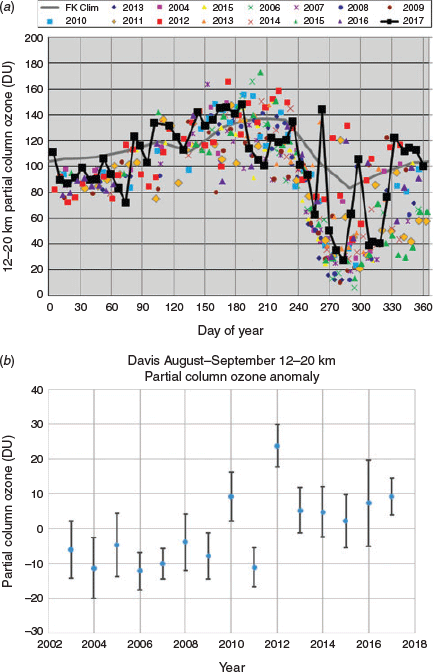
Figure A1.3 summarises 12- to 20-km partial column ozone values from measurements at Davis research station in Antarctica, whereas the Davis partial column values measured in July (days 180–212) and August (days 212–243) were mostly less than those of June (days 152–179), the overall June to August average was consistent with the long-term average since 2003 and also consistent with the value expected on the basis of the average surface SAM index value (see Krummel et al. (2019) for discussion of the relationship between with the winter SAM index and Davis 12–20 km partial column ozone). As can be seen in Fig. A1.3a, notable above-average anomalies in the 12–20 km partial column abundance occurred on September 20 (day 263) and October 18 (day 291) and 25 (day 298) – during these measurements, Davis was outside the edge of the polar vortex. The measurements on 20 September are discussed further below.
|
Figure A1.3b shows the August–September average anomaly for the Davis 12–20 km partial column ozone abundance over 2003–2017. These particular months are selected as, for this height range at Davis, they are generally during the period between the start and peak of maximum ozone depletion. To produce this figure, anomalies were evaluated from each measurement by subtracting a climatological function (consisting of a constant and annual and semiannual sinusoidal terms) that was fitted to all available data. Before averaging, anomalies outside ±2 standard deviations of the mean anomaly were rejected (consisting of three measurements, including that of 20 September 2017). The average value for 2017 was slightly above all other years except 2012, but within the 95% confidence limit of all years. In the context of the years shown in this figure, 2017 is the lowest ranked year in terms of the ozone hole metrics 1–6 provided in Table 1, and 2012 (which has the highest value in Fig. 1b) is the next nearest ranked year.
Figure A1.4 highlights the situation responsible for the anomalous 12–20 km partial column ozone measurement at Davis on 20 September. The ozone partial pressure profile for this day and the flights 1 week either side are shown in Fig. A1.4a. For 20 September, the estimated total column ozone abundance was the second largest observed at Davis (414 DU was recorded on 13 October 2012). The profile for this day contrasted with those obtained on 13 and 27 September for which the effects of the ozone hole was apparent in the height range 15 to ~22 km. In Figure A1.4b, it can be seen that on 20 September Davis was situated outside the ozone hole and under the mid-latitude ozone ridge. Trajectory modelling, shown in Fig. A1.4c, indicates that the air in the height range 18–23 km that was sampled at Davis on this day was generally outside the Antarctic continental boundary during the preceding 5 days, at times impinged on latitudes as far north as ~45°S.

|
A1.4 Antarctic ultraviolet radiation
Measurements of biologically effective solar ultraviolet (UV) radiation continued in 2017 at Casey (66.3°S and 110.5°E), Mawson (67.6°S and 62.9°E) and Davis research stations in Antarctica. Details on the instrumentation and methods used are provided by Tully et al. (2008) and Klekociuk et al. (2015).
Figure A1.5 shows the daily maximum UV radiation index for the three stations 2017, along with daily climatological time series for 2007–17. A feature of the Antarctic measurements during 2017 was the above-average levels during mid-November, which set new extreme high values at each station. These high levels occurred at the time when the mean UV Index time series tends to dip slightly for a period of 1–2 weeks when increasing ozone levels associated with breakdown of the ozone hole compensate for the decreasing zenith angle of the noon sun. Around the time of the high UV levels, the ozone hole was strongly asymmetric in shape and displaced off the pole towards East Antarctica. The pronounced asymmetry of the vortex from late October to mid-November is indicated by the anomalously large geopotential height zonal variation in Fig. 5.

|
A1.5 Ground-based infrared measurements
Figure A1.6 shows measurements of total column gas-phase abundances of ozone, nitric acid (HNO3), hydrochloric acid (HCl) and chlorine nitrate (ClONO2) above Arrival Heights, Antarctica (77.8°S, 166.7°E). These are obtained from solar mid-infrared spectroscopic measurements taken with a ground based Fourier transform spectrometer (Kohlhepp 2012). The ozone abundances for the spring of 2017 shown in Fig. A1.6a were, in common with other years, highly variable on daily to weekly timescales, reflecting the proximity of the site to the edge of the polar vortex (with lower values inside the vortex). All of the measured abundances during the ozone hole period of 2017 were above the minimum climatological values observed. Notable high ozone abundances were observed near days 265 (22 September, associated with the vortex distortion shown in Fig. A1.6b) and between days 305 and 315 (1–11 November, coinciding with a peak in the geopotential height anomaly at 70°S in Fig. 7).

|
The gas-phase abundance of HNO3 during spring generally exhibits similar day-to-day variability as ozone (Fig. A1.6b). The levels of this species are generally reduced over winter by incorporation into polar stratospheric cloud (PSC) particles; the sedimentation of these particles into the troposphere causes the denitrification of the lower stratosphere which enhances ozone loss in spring by slowing the partitioning of activated chlorine into the reservoir species ClONO2. A near record low measurement of the HNO3 abundance was obtained on 9 September (day 252) when the site was well inside the vortex, but there is no specific indication from these measurements that PSC volume or denitrification was particularly unusual in 2017. High HNO3 abundances from 22 October to 11 November (day 295 to 315) occurred when the site was outside the polar vortex (coinciding with peaks in the geopotential height anomaly at 75°S in Fig. 7).
The overall severity of ozone loss depends on the competition between deactivation, which repartitions chlorine into HCl and ClONO2, and activation, which frees up chlorine. Production of ClONO2 increases when gas-phase HNO3 is photolysed by sunlight, and the reaction of ClONO2 with HCl creates activated chlorine (Solomon et al. 2014). Above-average HCl in the lower stratosphere would be expected in 2017 on the basis of the inferred higher levels of Cly associated with the westerly phase of the QBO in 2017 discussed in Section 3.5. The abundance of HCl during September (days 244–273) shown in Fig. A1.6c was slightly above average at the times of the lowest ozone abundance measurements, which would be expected as the result of the chlorine activation reaction between HCl and ClONO2. The production of ClONO2 would be expected to be slowed by this activation reaction as well as by a reduction in HNO3 photolysis caused by enhanced denitrification. As can be seen in Fig. A1.6d, the abundance of ClONO2 in the postwinter measurements of 2017 was generally above average, and at record levels between days 255 and 265 (12 and 21 September). However, during this latter period, the site was situated outside the vortex. Representative periods when the site was inside the vortex were 7 September (day 250), 27 September (day 270), 17 October (day 290) and 16 November (day 320). Around 7 September, the ClONO2 abundance was similar to other years of measurements. For the other intervals, the ClONO2 abundance was above average, suggesting that the mitigation of ozone depletion by chlorine deactivation was higher than normal, and this is consistent with the generally reduced severity of ozone loss at these times compared with most recent years (refer to Fig. 1). As HNO3 abundances were not notably above average in the spring of 2017, nor were HCl abundances below average, the above-average ClONO2 levels within the vortex discussed above could have resulted from increased efficiency of HNO3 photolysis due to the level of distortion of the vortex allowing enhanced exposure to sunlight.