
Optical properties of Sydney aerosols
Gail P. Box A C and Taleb Hallal A BA School of Physics, University of New South Wales, Sydney, NSW 2052, Australia.
B Boral Cement, Taylor Avenue, Sydney, NSW 2577, Australia.
C Corresponding author. Email: gailpbox@gmail.com
Journal of Southern Hemisphere Earth Systems Science 69(1) 65-74 https://doi.org/10.1071/ES19001
Submitted: 6 December 2018 Accepted: 29 January 2019 Published: 11 June 2020
Journal Compilation © BoM 2019 Open Access CC BY-NC-ND
Abstract
Aerosol chemistry for PM2.5 and PM10 (particulate matter less than 2.5- and 10-μm aerodynamic diameter) samples collected in the Sydney region between November 2002 and December 2003 was used to estimate size-resolved refractive index for Sydney. Seasonal PM10–2.5 chemistry was obtained by subtracting seasonal PM2.5 from seasonal PM10 chemical composition. The chemical compounds present were determined from the elemental composition using two methods: the SCAPE 2 chemical thermodynamic model and aerosol types based on marker elements. Refractive index was then calculated using a mass fraction approach. Both methods agreed within the error bars indicating that useful optical properties can be derived from elemental chemistry. For the fine mode (PM2.5), the real component of the refractive index was 1.46 ± 0.07 with no seasonal variation, but there were seasonal variations in imaginary component, 0.05 ± 0.02 in summer and 0.23 ± 0.05 in spring. The coarse mode (PM10–2.5) real refractive index was constant throughout the year at 1.47 ± 0.09, whereas the imaginary refractive index was 0.01 ± 0.04 in summer and 0.04 ± 0.06 in spring. Representative refractive indices were then used to calculate aerosol scattering properties for three different size distributions to illustrate how this information could be used.
1 Introduction
Sunlight passing through the atmosphere is scattered and absorbed by the clouds, molecules and particles in the atmosphere. Scattering by molecules is responsible for the blue colour of the sky and the red of sunset. Scattering by clouds reduces incoming sunlight and makes cloudy days cooler. Scattering by aerosol particles is responsible for hazy days, especially in industrialized regions, as well as other subtle effects which can impact climate from the regional to the global level. Scattering and absorption by aerosol particles can affect visibility in some regions and must be taken into account when considering radiative forcing and climate impacts. To quantify effects such as visibility and radiative forcing, we need to know the aerosol optical properties such as the refractive index, scattering coefficient, absorption coefficient and asymmetry parameter. Aerosol refractive index is strongly dependent on aerosol chemistry, whereas the scattering coefficient, absorption coefficient and asymmetry parameter depend on both refractive index and aerosol size distribution. Aerosols are ubiquitous in the atmosphere but are highly variable in space and time, so local and regional knowledge of their properties is needed in order to evaluate their effects on air quality, health and their climate impacts such as radiative forcing for the particular region.
Aerosol chemical composition varies with location, for example between urban and rural areas, between coastal and inland regions. It can also vary with season: for example, the sea salt component on the coast will be affected by seasonal variations in onshore winds; black carbon (BC) from motor vehicles and fossil fuel burning may be elevated in winter due to domestic heating. Sea salt affects the scattering of light, whereas BC primarily affects absorption.
It is beyond the scope of this paper to provide an overview of methods used to determine aerosol scattering and absorption properties. Hand and Malm (2007) provide a review of ground-based measurements of aerosol scattering, whereas reviews of absorption measurements are given in Horvath (1993) and Bond and Bergstrom (2006). The focus of this paper is aerosol refractive index with the real part which is related to scattering, and the imaginary part which is related to absorption, treated separately.
Between November 2002 and December 2003 samples of PM2.5 and PM10 (particulate matter less than 2.5- and 10-μm aerodynamic diameter) aerosols were collected at four sites in the greater Sydney Basin. The objectives of this study were first to determine the spatial and seasonal variation of size-resolved aerosol chemical composition in the Sydney region (Hallal et al. 2013), and second to use the aerosol chemistry to determine aerosol refractive index for this region. This paper focuses on the second of these objectives, the determination of refractive index. Thence optical properties such as extinction efficiency, scattering and absorption efficiency, single scattering albedo and asymmetry parameter can be calculated.
Aerosol refractive index was determined from elemental chemistry using two methods: a chemical thermodynamic model and aerosol types. Refractive index was then determined for PM2.5, PM10 and PM10–2.5 (particulate matter between 2.5- and 10-μm aerodynamic diameter) size fractions, and their seasonal and spatial variations examined. Representative values of refractive index were then used with three different aerosol size distributions representative of Sydney to examine how aerosol extinction, asymmetry parameter and single scattering albedo vary with season and aerosol size distribution.
2 Methodology
2.1 Sample collection and analysis
A detailed description of the sampling and analysis for this study is given in Hallal et al. (2013), so only a brief outline is provided here. Sampling was carried out at four sites: Kensington, an urban area; Campbelltown, a semiurban area; Moss Vale, a rural–urban area and Berrima, a rural–industrial area (major cement plant and stock-feed mill). Kensington is close to both the coast and the Sydney central business district (CBD); Campbelltown is 45 km south-west of the Sydney CBD; Moss Vale and Berrima are both in the Southern Highlands south of Sydney, 140 and 130 km respectively from the Sydney CBD. These sites represent the different environmental, topographic and meteorological conditions in the Sydney region.
A total of 102 samples were collected on several days at each site in summer, autumn, winter and spring using an Ecotech MicroVol 1000 sampler with a flow rate of 3 L/min. The samples were collected on 47-mm Nuclepore Polycarbonate Membrane Filters with 1.0-μm pore size. Most samples were collected over a 24-h period, and on most days, a PM2.5 and a PM10 (particulate matter less than 2.5- and 10-μm aerodynamic diameter) sampler were run side by side in order to identify size-related differences in composition.
The elemental composition of the samples was determined using the accelerator-based ion beam analysis (IBA) techniques, proton-induced X-ray emission (PIXE) and proton-induced gamma-ray emission (Cohen et al. 2004) at the Australian Nuclear Science and Technology Organisation (ANSTO). BC was determined using the Laser Integrating Plate Method (Taha et al. 2007).
2.2 Determination of chemical composition
In order to determine the refractive index of the atmospheric aerosol, it is necessary to know which compounds are present in the air. Two methods have been applied to the elemental composition data to determine the chemical compounds present. The simplest method uses marker elements to determine aerosol types. The second method is a chemical thermodynamic model which uses ionic composition and thus required some assumptions to be made. Both methods are described below.
2.2.1 Aerosol types
In Hallal et al. (2013) elemental chemistry was used to determine typical aerosol types, based on Malm et al. (1994). It would also be suited to large data sets and ongoing monitoring.
Aerosols can be classified into a number of major types: sea salt, sulfates, nitrates, soil, organics and light-absorbing carbon (Malm et al. 1994). For each aerosol type the elemental concentration of its marker element is multiplied by a scaling factor obtained by dividing the total molar weight of the aerosol type by the atomic weight of the marker element. The type definitions used are given below:
Sea salt = 2.54 × [Na]
Soil = 2.2 × [Al] + 2.49 × [Si] + 1.63 × [Ca] + 1.94 × [Ti] +2.42 × [Fe]
Sulfate = 4.125 × [S]
Smoke = [K] − 0.6 × [Fe]
Square brackets in the above equations indicate element concentrations. Sulfate was assumed to be fully neutralised and found as (NH4)2SO4. BC (also called light-absorbing carbon) was found using the Laser Integrating Plate Method (Taha et al. 2007). Since no measurements of O, H or N were available for this study, [water + nitrates] was assumed to be 16% of total mass (Cohen et al. 1995). Organic was then estimated as

For each sample the mass of each aerosol type was calculated from the measured elemental composition, and from this, the percentage of total sample mass accounted for by each aerosol type was obtained.
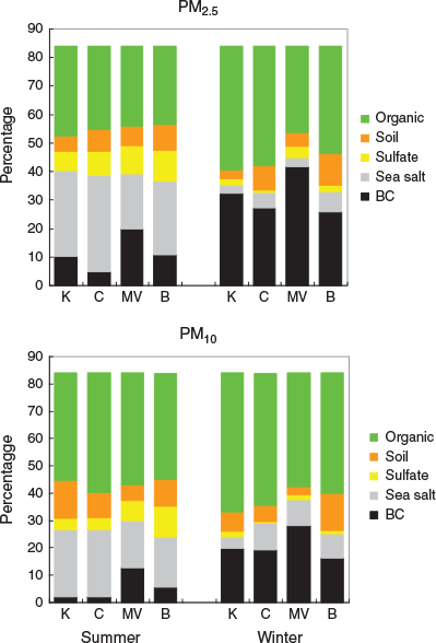
The summer and winter average PM2.5 and PM10 aerosol composition for each site are illustrated in Fig. 1. It is evident that there are seasonal variations in aerosol composition. Sea salt and sulfate account for a higher fraction of total aerosol in summer (left-hand panel) than in winter (right-hand panel) for both PM2.5 (top row) and PM10 (bottom row). For BC there are distinct seasonal variations for all sites, and it accounts for a greater fraction of PM2.5 than PM10. More detailed discussion of aerosol types is given in Hallal et al. (2013).
|
2.2.2 Thermodynamic model
The SCAPE 2 chemical equilibrium thermodynamic model (Kim et al. 1993a, 1993b; Kim and Seinfeld 1995; Meng et al. 1995) was used to estimate the state and composition of inorganic species in the aerosol phase. The model assumes a system of ammonium, chloride, nitrate, sodium, sulfate, calcium, potassium, magnesium and carbonate ions and water which exists in solid and liquid phases. Given the concentration of the respective ions for a mixture of water-soluble inorganic particles, relative humidity (RH) and temperature as an input, the model calculates the equilibrium physical state and composition of the mixture. For the current study the program returned mass concentration of ions and compounds present at ambient temperature and RH. The necessity of assuming equivalence between ionic and elemental composition is a source of error. Errors are discussed below after the discussion of refractive index calculations.
The model was run for each PM2.5 and PM10 sample (daily mass) as well as for seasonal and year average PM2.5 and PM10 (average mass) at each site. Since a major focus of this work was to obtain size-resolved optical properties, coarse mode elemental composition (PM10–2.5) was determined by subtracting seasonally averaged PM2.5 from seasonally averaged PM10 concentrations. These values were then used as input to SCAPE 2.
The output from SCAPE 2 represents the soluble component of the aerosol. BC and soil were as defined above. Organic mass was then determined by subtracting soluble mass, soil and BC from total mass.
2.3 Determination of aerosol refractive index
Aerosol refractive index was calculated using a mass fraction approach. Refractive index, n, is given by

where mi is the mass of the ith compound, ni is its refractive index and M is total sample mass.
The refractive indices used in these calculations were taken from the literature (Weast 1975, 1977; Stelson 1990; Morrison and Boyd 1978; Lide 1997; Evans 2003; Aylward and Findlay 2008). The refractive index for organics was assumed to be 1.4 (Turpin and Lim 2001), and for BC it was assumed to be 1.5 (Lide 1997). The imaginary component of refractive index of BC was taken as 0.47 (Horvath 1993) because these particles occur as a mixture of soot and air. The reference refractive index of soluble substances (ions) was taken from the literature (Stelson 1990; Moelwyn-Hughes 1961).
Refractive index was determined for each day at each site (daily mass), and from these values seasonal and yearly averages were calculated. A second set of calculations was done using average chemistry (average mass) for the season or year, in order to determine whether or not using average chemistry has a significant effect on the result.
2.4 Sources of error
In order to use elemental chemistry as input to SCAPE 2, it was assumed that the ionic concentration was the same as the elemental concentration. However, SCAPE 2 is based on soluble ions, whereas total elemental concentration will include both soluble and insoluble fractions. Since no soluble ion chemistry was available to this study, the uncertainty introduced by these assumptions was estimated using values for the Sydney region taken from the literature. Nitrates were assumed to be 8% of total mass (Cohen et al. 1995). Total carbonate concentration as H2CO3 was calculated using a CO2 global average concentration of 360 ppm (Meng et al. 1995).
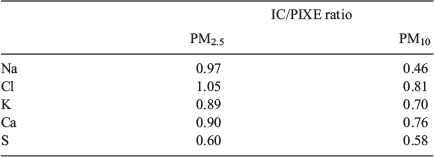
Ayers et al. (1999) measured both elemental and ion concentrations (ICs) of aerosol samples in Sydney as part of the Australian Fine Particle study. For Na, Cl, K, Ca and S, a multiplicative factor, the ratio of IC to elemental concentration (from PIXE), was determined for both PM2.5 and PM10. These ratios are given in Table 1. The ion/element ratios for Na, Cl, K, Ca and S indicated that 95% of PM2.5 and 68% of PM10 was soluble.
|
The low mass concentration of samples in this study meant that Mg was below the minimum detectable limit for IBA, so was assumed to be zero in the SCAPE 2 runs. To estimate the level of error introduced by this assumption, the concentration of soluble Mg ions was taken from Ayers et al. (1999) for both PM2.5 and PM10, whereas elemental Mg for PM2.5 was taken from PIXE results for Christchurch obtained by Senaratne et al. (2005).
Two representative data sets were selected for the test, a PM2.5 summer and PM10 winter. For both test data sets, SCAPE 2 was run for ions input with and without Mg, and also elemental input data with Mg. Real refractive index was calculated for the test cases, and these were compared with the original estimates. It was found that using the ions output without Mg resulted in a refractive index ~3% higher than with elements as input. When Mg is also included, the refractive index is ~10% higher.
3 Results
The primary purpose of this study was to determine the size-resolved refractive index for the Sydney region, including seasonal and spatial variations, which are discussed in Section 3.1. In Section 3.2 we illustrate some potential applications of this approach.
3.1 Refractive index
In this study measured elemental chemistry has been used to determine the size-resolved refractive index for the Sydney region and to examine its seasonal and spatial variations. For each sample, the chemical compounds present have been derived from the elemental composition using both a chemical thermodynamic model and aerosol types. This resulted in two sets of refractive indices.
The analysis of the data was motivated by the following questions: (1) Does seasonally averaged chemistry give reliable results? (2) Are there seasonal or site variation in refractive index? and (3) Is refractive index based on aerosol types comparable to that based on the chemical thermodynamic model? To answer these questions, the seasonal average and standard deviation of daily samples, referred to as daily mass, was calculated for each site. This was done for PM2.5 and PM10 samples for both data sets. The final results of these calculations are summarised in Table 2. The full results are given in the Appendix 1, along with the corresponding refractive indices based on seasonally averaged chemistry (referred to as average mass).
|
3.1.1 Real component of refractive index
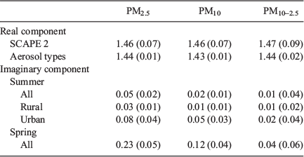
For each data set the real refractive index based on seasonally averaged mass agreed with that based on daily mass within one standard deviation for both PM2.5 and PM10 in the vast majority of cases. (See Table A1.1 of Appendix 1 for detailed results.) Comparison of PM2.5 and PM10 seasonal refractive indices showed that the differences between sites, and also between seasons, were small and less than the seasonal error bars. This leads to the conclusion that seasonally averaged chemistry gives reliable estimates of real refractive index and that the seasonal and spatial variations were not significant.
Table 2 provides the average PM2.5 and average PM10 refractive index over all sites and seasons for both SCAPE 2 and aerosol types. The PM2.5 and PM10 refractive indices based on aerosol types are slightly smaller than for SCAPE 2, but the difference is not significant. Benko et al. (2009) obtained similar results for Central European background aerosol which showed no significant variation in refractive indices between the seasons.
Comparison of refractive indices calculated from aerosol types and those calculated from SCAPE 2 showed good agreement for seasonally averaged daily mass and average mass for all sites and seasons. The standard deviations for the aerosol types were smaller than for SCAPE 2 which may reflect the limited range of aerosol types plus the assumption of constant 16% total mass for (water + nitrates). (Aerosol types allow only one sulphate, for example, whereas SCAPE 2 allows several; however, refractive indices for most compounds are in the range 1.50 ± 0.05, so the effect is small.)
3.1.2 Imaginary component of refractive index
Calculation of the imaginary component of the refractive index depends only on BC concentration and is the same for both aerosol types and SCAPE 2. Results are summarised in Table 2. (See Table A1.2 of Appendix 1 for detailed results.) In the vast majority of cases, the imaginary refractive index based on seasonally averaged mass agreed with that based on daily mass within the seasonal error bars. There was significant seasonal variation in the imaginary part of the refractive index, some variation between sites and also variation with size fraction. The lowest values at all sites occurred in summer and the highest in spring (and winter), and in most cases, the PM10 value is lower than the PM2.5 value. Table 2 shows the average refractive index over all sites for summer and spring for both PM2.5 and PM10. Refractive index averaged over all sites is significantly lower in summer than in spring for both PM2.5 and PM10. Also shown are the summer averages for the urban (Kensington and Campbelltown) and rural (Moss Vale and Berrima) sites. The urban refractive index was significantly lower than the rural for both PM2.5 and PM10. For spring, there were no significant differences between urban and rural sites. The differences in imaginary refractive index with size fraction reflect the stronger contribution of BC to PM2.5.
3.1.3 Size-resolved refractive index
From the results presented above, it is evident that a good estimate of refractive index can be obtained using seasonally averaged chemistry for both PM2.5 and PM10. This suggests that using coarse mode chemistry obtained by subtracting seasonal PM2.5 from seasonal PM10 to estimate coarse mode (PM10–2.5) refractive index should provide useful results. The coarse mode (PM10–2.5) refractive index was calculated for both SCAPE 2 and aerosol types and the error estimated as the square root of sum squares of the corresponding PM2.5 and PM10 errors. The results for the coarse (PM10–2.5) fractions are summarised in Table 2. (See Table A1.3 of Appendix 1 for detailed results.) There are some small seasonal variations in real refractive index between seasons and between sites for PM10–2.5, most noticeably Kensington and Berrima, but these are unlikely to be significant. The real refractive index averaged over all sites is the same as the corresponding PM10 value for both SCAPE 2 and aerosol types.
There are slight variations in imaginary component of the refractive index for the coarse fraction, and this is reflected in the slightly higher value in spring than summer shown in Table 2. PM10–2.5 values are also lower than the corresponding PM10, particularly for spring. The imaginary component is higher for PM2.5 than for PM10–2.5, even when errors are accounted for, reflecting the greater contribution of BC to the fine fraction. The real component of PM10–2.5 refractive index is 1.47 ± 0.09 throughout the year and the imaginary component is 0.01 ± 0.04 for summer and 0.04 ± 0.06 for spring.
The good agreement between the results derived from the two data sets suggests that estimating aerosol refractive index based on aerosol types can give reliable results and could be very useful when only elemental composition is available. For cases where there are sufficiently large data sets available, more sophisticated analysis, using positive matrix factorisation for example, would allow more accurate determination of the aerosol types present. This in turn would allow more accurate estimates of refractive index for that location.
3.2 Application of refractive index results
3.2.1 Aerosol scattering properties definitions
Aerosol optical properties which depend on aerosol refractive index include the extinction and scattering efficiencies, single scattering albedo and the asymmetry parameter. Brief definitions are given here, and more details can be found in Box and Box (2016). The extinction efficiency, βe, is a measure of the attenuation of the beam due to both absorption and scattering, whereas the scattering efficiency, βs, is a measure of attenuation due to scattering. These are defined as:
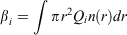
where i = e and s, for extinction and scattering respectively.
Qi is the Mie extinction or scattering coefficient and n(r) is the aerosol size distribution. It should be noted that Qi is a function of particle size, refractive index and wavelength.
The single scatter albedo ϖ provides a measure of how well a population of particles scatters incident light, ϖ = 1 for a perfect scatterer and ϖ = 0 for a perfect absorber. It is defined as:
The asymmetry parameter g gives a measure of the directionality of the scattered beam, g = 0 being uniformly scattered in all directions and g = 1 being highly directional. It is defined as:
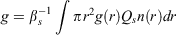
where g(r) is the asymmetry parameter for an individual particle of radius r.
The size distributions used to calculate the optical properties were modelled as bimodal lognormal distributions with a fine mode corresponding to PM2.5 and a coarse mode corresponding to PM10–2.5. Each mode has the form:
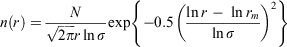
where n(r) is the radius-number size distribution, N is the total number of particles per unit volume, rm is the geometric mean radius and σ is the size distribution geometric standard deviation.
3.2.2 Aerosol scattering properties calculations
Aerosol optical properties depend on both refractive index and size distribution. In this section we examine the seasonal and spatial variations of aerosol scattering properties for the Sydney region. This illustrates a potential application of refractive index determination using aerosol chemistry.
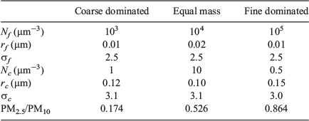
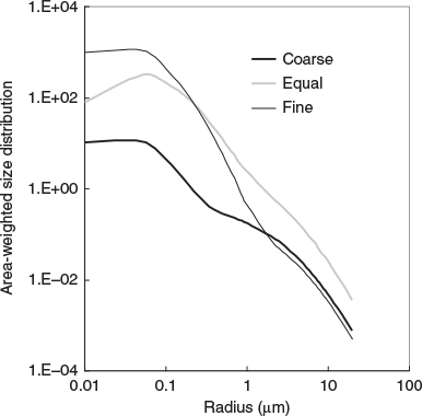
A set of three size distributions was constructed based on measured size distributions for the Sydney area. This ensured that the values chosen for geometric mean radius (rm) and geometric standard deviation (σ) for both fine and coarse modes were appropriate for Sydney. Model parameters were chosen to give one size distribution where the fine mode dominated the mass, one with roughly equal fine and coarse mass, and a third where the coarse mode dominated the total mass. The size distribution parameters and PM2.5/PM10 ratios are given in Table 3. The area-weighted distribution r2n(r) (units: μm2 μm−3 μm−1) is the most relevant representation for calculation of scattering properties and is illustrated in Fig. 2.
|
|
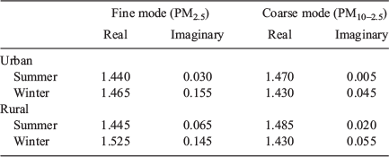
To examine variations in scattering properties, the PM2.5 and PM10–2.5 summer and winter refractive indices for Kensington and Campbelltown were averaged to give representative seasonal urban values, and similarly Moss Vale and Berrima were averaged to give seasonal rural values. These refractive indices are given in Table 4. The variation of extinction, asymmetry parameter and single scattering albedo as a function of wavelength for each size distribution is illustrated in Fig. 3.
|

|
It is evident from Fig. 3 that the size distribution has an effect on the behaviour of scattering properties as a function of wavelength. The curves for the coarse mass dominated size distribution (left column) were the flattest and those for the fine mass dominated size distributions (right column) were the steepest.
Extinctions (top row) have been normalised to 1 at 0.5 μm to enable easy comparison of shape as a function of wavelength. There is very little difference between urban (black) and rural (grey) extinctions for a given size distribution but there are seasonal and size distribution differences. As noted above the coarse mass dominated size distribution is the flattest, and there are no seasonal differences between normalised extinctions. For the other two size distributions, the winter extinctions (dashed lines) are higher than summer (solid lines) at longer wavelengths and the effect is more pronounced for the fine mass dominated distribution.
The asymmetry parameter (middle row) shows seasonal, spatial and size distribution differences. For the coarse dominated size distribution the rural summer and winter asymmetry parameters are constant with wavelength at ≈0.8, whereas the urban values are slightly higher in winter and lower in summer. Seasonal and spatial differences for the size distribution with equal fine and coarse mass were small, whereas for the fine mass dominated distribution asymmetry parameters decreased with wavelength and the effect was more pronounced for winter reflecting the increased absorption.
The seasonal, spatial and size distribution differences for single scatter albedo (bottom row) are most pronounced. A common feature for all three size distributions was that the difference between summer and winter values is greater for the urban case than for the rural case at all wavelengths. The summer urban values are higher than the rural ones, but the opposite is the case for winter.
4 Summary and conclusion
In this paper we have used the aerosol chemistry for the Sydney region, presented in Hallal et al. (2013), to estimate size-resolved refractive index for Sydney. The chemical compounds present were determined from the elemental composition using two methods: the SCAPE 2 chemical thermodynamic model and aerosol types based on marker elements. Refractive index was then calculated using a mass fraction approach. Representative refractive indices were then used to calculate aerosol scattering properties for three different size distributions to illustrate how this information could be used. The key findings are summarised below.
For both PM2.5 and PM10 it was found that the results based on seasonally averaged chemistry were within one standard deviation of the seasonally averaged daily data, and generally much closer, indicating that averaged chemistry does lead to a representative value for refractive index.
There was little seasonal or site variation in the real part of the refractive index which was found to be 1.46 ± 0.07 for both PM2.5 and PM10. The urban sites (Kensington and Campbelltown) tended to have slightly lower values than the rural sites (Moss Vale and Berrima) but the differences were not significant.
The imaginary component of the refractive index showed strong variations with season, site and particle size. Lowest values were in summer and highest in spring. For PM2.5 the summer average was 0.05 ± 0.02 (urban 0.03 ± 0.01, rural 0.08 ± 0.04) and the spring average was 0.23 ± 0.05. For PM10 the summer average was 0.02 ± 0.01 (urban 0.01 ± 0.01, rural 0.05 ± 0.03), whereas the spring average was 0.12 ± 0.04.
The real part of the coarse mode (PM10–2.5) refractive index showed little seasonal or site variation and was found to be 1.47 ± 0.09. This is the same as for PM2.5 and PM10. The imaginary component for the coarse mode was 0.01 ± 0.04 in summer and 0.04 ± 0.06 in spring. This was much lower than that for the fine mode and, unlike PM2.5 and PM10, seasonal and site variations were small and not significant. The lower imaginary component for PM10–2.5 indicates that BC is predominantly in the fine mode.
The values quoted above for real refractive index may be underestimates due to the assumptions made about the equivalence of elemental and ionic composition and the neglect of Mg. This source of error is of the order of 10%.
Refractive indices based on aerosol types were comparable to those based on SCAPE 2 and indicate that using elemental composition to determine aerosol types, and thence refractive index, is a reliable approach.
The most significant contributor to variations in refractive index (real and imaginary) is BC due to its strong seasonal variability. It should also be noted that there is a wide variation in refractive index for BC in the literature depending on its source, for example pure soot or a soot/air mixture, and mixture proportion. This will affect comparisons with other studies.
The results outlined above were used to calculate aerosol scattering properties for the Sydney region, specifically extinction, asymmetry parameter and single scatter albedo, as a function of wavelength. Three size distributions and four different refractive indices were used to investigate the effects of differing fine/coarse mode mass ratios as well as seasonal and spatial variations. Extinction decreased with wavelength for all three size distributions with the effect being strongest for the fine mass dominated distribution. Wavelength dependence of the asymmetry parameter and single scatter albedo was also strongest for the fine mass dominated distributions. Single scatter albedo showed the greatest variation between rural and urban sites, and also with season, for all three size distributions. Only extinction, single scattering albedo and asymmetry parameter were considered here because of large uncertainties in refractive index, and the representative nature of the size distributions did not justify extending the application to more sophisticated radiative forcing calculations which would also require column loadings.
In this study elemental chemistry has been used to determine the refractive index for the Sydney region. We have demonstrated that the simplified method based on aerosol types gives comparable results to those based on the thermodynamic model. The simplified method may be preferable when only elemental composition data is available because it avoids introducing errors arising from assumptions about ion/element ratios. These assumptions affected the accuracy of the real part of the refractive index rather than the imaginary part which contributed most strongly to variability for the sites studied. There are separate issues regarding what values to use for BC refractive index, and these will depend on local factors and sources.
This study has shown that useful information about aerosol optical properties can be derived from limited data. In this case fine and coarse mode refractive index was determined from elemental composition of aerosol samples collected on two low volume samplers (PM2.5 and PM10). Two major improvements to the procedure used here are recommended for future studies: a two-stage (or multi-stage) sampler and a high flow rate. In a two-stage sampler the same air passes through both stages separating the coarse and fine particles, thus eliminating the major source of error arising from the determination of the coarse mode by subtracting PM2.5 from corresponding PM10. A multi-stage sampler would allow for better size resolution of chemistry and hence refractive index. High flow rates would lead to increased mass on filters resulting in more accurate elemental chemistry by ensuring that mass concentrations were above the minimum detectable limit for all elements.
Acknowledgements
The elemental chemistry analyses that formed the basis of this paper were done at ANSTO under AINSE grants AINGRA03178 and AINGRA08005.
References
Ayers, G. P., Keywood, M. D., Gras, J. L., Cohen, D. D., Garton, D., and Bailey, G. M. (1999). Chemical and physical properties of Australian fine particles: a pilot study. Final report to Environment Australia from the Division of Atmospheric Research, CSIRO and the Australian Nuclear Science and Technology Organisation. (CSIRO: Australia.)Aylward, G., and Findlay, T. (2008). ‘SI Chemical Data’, 6th edn. (John Wiley & Sons, Ltd.: Milton, Qld, Australia.)
Benko, D., Molnar, A., and Imre, K. (2009). Study on the size dependence of complex refractive index of atmospheric aerosol particles over Central Europe. IDŐJÁRÁS 113, 157–175.
Bond, T. C., and Bergstrom, R. W. (2006). Light absorption by carbonaceous particles: an investigative review. Aerosol. Sci. Tech. 40, 27–67.
| Light absorption by carbonaceous particles: an investigative review.Crossref | GoogleScholarGoogle Scholar |
Box, M. A., and Box, G. P. (2016). ‘Physics of Radiation and Climate’. (CRC Press: Boca Raton, FL, USA.)
Cohen, D. D., Crisp, P. T., and Hyde, R. (1995). Contribution of fuel combustion to pollution by airborne particles in urban and non-urban environments. Report number ERDC 259. (Energy Research and Development Corporation: Canberra.)
Cohen, D. D., Stelcer, E., Hawas, O., and Garton, D. (2004). IBA methods for characterization of fine particulate atmospheric pollution: a local, regional and global research problem. Nucl. Instrum. Meth. B 219–220, 145–152.
| IBA methods for characterization of fine particulate atmospheric pollution: a local, regional and global research problem.Crossref | GoogleScholarGoogle Scholar |
Evans, M. C. F. (2003). Characterization and formation of particulate nitrate in a coastal area. PhD Thesis. Department of Chemistry, College of Arts and Sciences, University of South Florida, USA.
Hallal, T., Box, G. P., Cohen, D. D., and Stelcer, E. (2013). Size-resolved elemental composition of aerosol particles in greater Sydney in 2002-2003. Environ. Chem. 10, 295–305.
| Size-resolved elemental composition of aerosol particles in greater Sydney in 2002-2003.Crossref | GoogleScholarGoogle Scholar |
Hand, J. L., and Malm, W. C. (2007). Review of aerosol mass scattering efficiencies from ground-based measurements since 1990. J. Geophys. Res. 112, D16203.
| Review of aerosol mass scattering efficiencies from ground-based measurements since 1990.Crossref | GoogleScholarGoogle Scholar |
Horvath, H. (1993). Atmospheric light absorption – a review. Atmos. Environ. 27A, 293–317.
| Atmospheric light absorption – a review.Crossref | GoogleScholarGoogle Scholar |
Kim, Y. P., Seinfeld, J. H., and Saxena, P. (1993a). Atmospheric gas-aerosol equilibrium I. Thermodynamic model. Aerosol Sci. Technol. 19, 157–181.
| Atmospheric gas-aerosol equilibrium I. Thermodynamic model.Crossref | GoogleScholarGoogle Scholar |
Kim, Y. P., Seinfeld, J. H., and Saxena, P. (1993b). Atmospheric gas-aerosol equilibrium II. Analysis of common approximation and activity coefficient calculation methods. Aerosol Sci. Technol. 19, 182–198.
| Atmospheric gas-aerosol equilibrium II. Analysis of common approximation and activity coefficient calculation methods.Crossref | GoogleScholarGoogle Scholar |
Kim, Y. P., and Seinfeld, J. H. (1995). Atmospheric gas-aerosol equilibrium III. Thermodynamics of crustal elements Ca2+, K+, and Mg2+. Aerosol Sci. Technol. 22, 93–110.
| Atmospheric gas-aerosol equilibrium III. Thermodynamics of crustal elements Ca2+, K+, and Mg2+.Crossref | GoogleScholarGoogle Scholar |
Lide, D. R. (1997). ‘Handbook of Chemistry and Physics.’ (CRC Press: Boca Raton, FL, USA.)
Malm, W. C., Sisler, J. F., Huffman, D., Eldred, R. A., and Cahill, T. A. (1994). Spatial and seasonal trends in particle concentration and optical extinction in the United States. J. Geophys. Res. 99, 1347–1370.
| Spatial and seasonal trends in particle concentration and optical extinction in the United States.Crossref | GoogleScholarGoogle Scholar |
Meng, Z., Saxena, P., and Kim, Y. P. (1995). Atmospheric gas-aerosol equilibrium IV. Thermodynamic of carbonates. Aerosol Sci. Technol. 23, 131–154.
| Atmospheric gas-aerosol equilibrium IV. Thermodynamic of carbonates.Crossref | GoogleScholarGoogle Scholar |
Moelwyn-Hughes, E. A. (1961). ‘Physical Chemistry.’ 2nd revised edn. pp. 397–400. (Pergamon Press: New York, NY, USA.)
Morrison, R. T., and Boyd R. N. (1978). ‘Organic Chemistry.’ 3rd edn. (New York University, Allyn and Bacon Inc.: Boston, MA, USA.)
Senaratne, I., Kelliher, F. M., and Triggs, C. (2005). Source apportionment of airborne particles during winter in contrasting coastal cities. Aerosol Air Qual. Res. 5, 48–64.
| Source apportionment of airborne particles during winter in contrasting coastal cities.Crossref | GoogleScholarGoogle Scholar |
Stelson, A. W. (1990). Urban aerosol refractive index prediction by partial molar refraction approach. Environ. Sci. Technol. 24, 1676–1679.
| Urban aerosol refractive index prediction by partial molar refraction approach.Crossref | GoogleScholarGoogle Scholar |
Taha, G., Cohen, D. D., Stelcer, E., and Box, G. P. (2007). Black carbon measurement using Laser Integrating Plate Method. Aerosol Sci. Tech. 41, 266–276.
| Black carbon measurement using Laser Integrating Plate Method.Crossref | GoogleScholarGoogle Scholar |
Turpin, B. J., and Lim, H. J. (2001). Species contributions to PM2.5 mass concentrations: revisiting common assumptions for estimating organic mass. Aerosol Sci. Technol. 35, 602–610.
| Species contributions to PM2.5 mass concentrations: revisiting common assumptions for estimating organic mass.Crossref | GoogleScholarGoogle Scholar |
Weast, R. C. (1975). ‘Handbook of Chemistry and Physics.’ 56th edn. (CRC Press: Cleveland, OH, USA.)
Weast, R. C. (1977). ‘Handbook of Chemistry and Physics.’ 57th edn. (CRC Press: Cleveland, OH, USA.)
Appendix 1. Full aerosol refractive index results.

|

|

|