
Experimental assimilation of synthetic bogus tropical cyclone pressure observations into a high-resolution rapid-update NWP model
Susan Rennie A B and Jim Fraser AA Australian Bureau of Meteorology, GPO Box 1289, Melbourne, Vic. 3001, Australia.
B Corresponding author. Email: susan.rennie@bom.gov.au
Journal of Southern Hemisphere Earth Systems Science 70(1) 215-224 https://doi.org/10.1071/ES19036
Submitted: 20 November 2019 Accepted: 3 June 2020 Published: 28 August 2020
Journal Compilation © BoM 2020 Open Access CC BY-NC-ND
Abstract
The effect of synthetic ‘bogus’ tropical cyclone (TC) central pressure observations on TC Owen was tested in a convective-scale numerical weather prediction (NWP) system with hourly 4D-Var assimilation. TC Owen traversed the Gulf of Carpentaria over 10–14 December 2018, entering from the east and briefly making landfall on the western edge before reversing course and retracing its path east to cross the northern tip of Queensland. The Australian Bureau of Meteorology runs a high-resolution NWP model centred over Darwin, which covers much of the Gulf of Carpentaria. The next-generation developmental version of this model includes data assimilation. Therefore, when TC Owen presented the opportunity to investigate the simulation of a TC within the domain, the developmental system was run as a case study. The modelled cyclone initially failed to intensify. The case study was then repeated including assimilation of bogus central pressure observations. This new run showed a large improvement in the intensity throughout the simulation; however, the TC track was not substantially improved. This demonstration of the potential impact of using synthetic observations may guide whether the development of a bogus observation source with sufficiently low latency for use in an hourly-cycling system should be prioritised.
Keywords: Australian cyclones, central pressure observations, convective-scale numerical weather prediction, data assimilation, Gulf of Carpentaria, synthetic observations, TC Owen, tropical cyclone.
1 Introduction
The Australian Bureau of Meteorology runs six high-resolution numerical weather prediction (NWP) configurations (1.5-km grid spacing) covering the major population areas of the country, the ‘City’ versions of ACCESS (Australian Community Climate and Earth System Simulator, Puri et al. 2013). Occasionally, tropical cyclones (TCs) occur in or pass through the Darwin domain, which covers the top end of the Northern Territory. The current operational high-resolution City NWP domains (Bureau National Operations Centre 2018) are run downscaled from the regional model (12-km grid spacing) that covers the Australasian region (ACCESS-R; Bureau National Operations Centre 2016), initialised every 6 h. However, a warm-running rapid-update NWP system with hourly 4D-Var data assimilation is currently being developed to replace the downscaling system as the operational high-resolution NWP in 2020.
During the development of the new ACCESS-City systems, a request was made to initialise the Darwin domain (ACCESS-DN) for the duration of TC Owen, so that forecasters could view some of the new NWP output diagnostics in the presence of a cyclone. TC Owen was predicted to enter the Gulf of Carpentaria from the east, and travel west for a period while intensifying, before reversing course and passing eastward back across the northern tip of Queensland. ACCESS-DN covers three-quarters of the Gulf of Carpentaria.
It became apparent during this run that the model did not adequately represent the TC intensity, likely due to a lack of observations to inform the model about the TC structure. Hence the warm-running version might compare poorly to the existing operational downscaler, which benefits from re-initialising every 6 h from ACCESS-R. This regional model has 6-h 4D-Var with a larger domain and satellite observation input, and consequently may better represent cyclone central pressure and location. In comparison, the warm-running ACCESS-City relies on a smaller set of observations (due to its smaller domain and time window) to analyse the cyclone, especially once it is away from the boundaries where ACCESS-R provides information. It was decided to rerun the period, including synthetic central pressure observations, with the objective of analysing the model response to this additional information about the TC. This allowed a controlled experiment of observation impact.
TCs often originate over tropical oceans where meteorological observations are frequently insufficient to accurately define vortex location and structure, particularly of the inner core. Synthetic observations (commonly known as bogus observations) derived from forecaster estimates of TC properties are often used in operational models (e.g. ACCESS-TC and the UK Met Office global model) to help improve TC analyses and forecasts. In addition to using all available conventional observations, the current operational 12-km ACCESS-TC Tropical Cyclone regional version of ACCESS (Bureau National Operations Centre 2017) uses a radial array of 123 bogus surface pressure observations based on manual forecaster estimates of TC position, central pressure and size to help specify the vortex position and structure (Davidson et al. 2014). A new developmental ACCESS-TC version (National Operations Centre 2020) will run at 4-km horizontal grid spacing and similarly assimilates a radial array of bogus observations. In contrast, the UK Met Office global model (Heming 2016) and also the latest ‘APS3’ (third generation Australian Parallel Suite) version of the Bureau of Meteorology’s global model (National Operations Centre 2019) assimilate only singular hourly central pressure bogus observations derived from international TC advisories. These observations are interpolated to hourly intervals between the available advisories, assuming there is more than one, and extrapolates up to 2 h past the final advisory. For simplicity, these hourly central pressure bogus observations were used in the ACCESS-DN experiments, rather than full radial arrays which were only available every 6 h.
Although within the last decade it has become more common for TC forecasts to be run at resolutions of 5 km or less, there has been little work done at <2 km resolution, the convection-permitting scales. This is due to the computational expense of running a large domain that can capture the lifetime of a TC. Experiments using bogus observations at these resolutions are similarly rare.
There are several caveats to be noted for this experiment. Firstly, the developmental ACCESS-City system is not in its final form. Although no major changes are expected for the NWP component, the operational data assimilation may include additional observations, and updated background covariances used by the 4D-Var. Therefore, the data assimilation is expected to be improved in future. Secondly, the source of the bogus observations are TC advisories released every 6 h, around 1–3 h after the valid time which is usually either 00, 06, 12 or 18 UTC. As the hourly 4D-Var relies on a latency (the delay after which observations are received) of at most 1 h, in real time the TC advisories would generally arrive too late. The value of this experiment is that it can show how much value such additional observations can add, and if it is worth pursuing a bogus observation source with lower latency.
2 TC Owen
The following description of TC Owen gives all times in UTC.
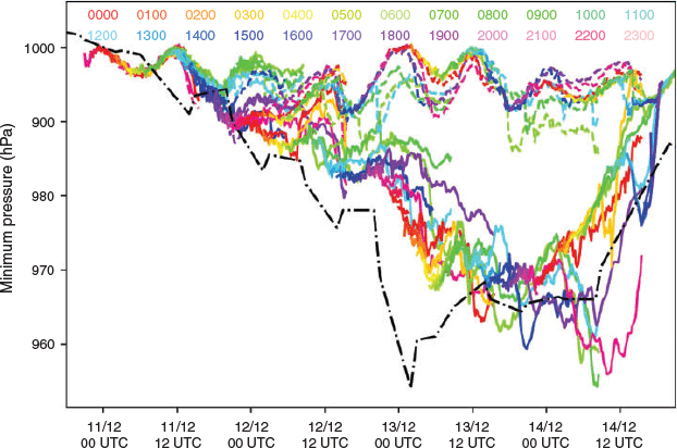
TC Owen formed in the northern Coral Sea on 2 December 2018 and reached category 2 before making its way westward while de-intensifying to a tropical low. It crossed the northern tip of Queensland at Port Douglas on 9 December as a tropical low and entered the Gulf of Carpentaria late on 10 December. As it travelled westward, it re-intensified to category 1 on 11 December, category 2 by 12 December and category 3 by 13 December. At this stage it had crossed the Gulf to touch land before turning and returning eastwards. TC Owen lost strength and made landfall back on the Queensland coast as a category 2 cyclone late on 14 December, and traversed Cape York back to the Coral Sea, rapidly returning to a tropical low. Fig. 1 shows TC Owen’s path, at 6-h intervals, with the day of month marked at the 00 UTC point. The TC locations are taken from the TC advisories published by the Bureau of Meteorology.

|
3 Method
The developmental ACCESS-City uses a stretched grid, with a uniform resolution central region of 0.0135° (~1.5 km) which then stretches out to 0.036° (~4 km) at the boundaries (Fig. 1). This is intended to improve the transmission of information from the coarser-resolution parent model through the lateral boundaries, and also to move boundary effects away from the inner region that will be used by forecasters. The grid has 80 vertical levels up to 38.5 km, with higher resolution near the surface and terrain-following coordinates. For this experiment the grid is nested inside the operational ACCESS-R, which is also used to initialise the run. This ‘cold start’ initialisation is done a couple of days before the event to allow for spin-up. Soil moisture is updated daily from the operational global ACCESS version, and sea surface temperatures are updated daily from RAMSSA (Regional Australian Multi-Sensor Sea surface temperature Analysis, Beggs et al. 2011).
The NWP component uses the Met Office Unified Model based on version 10.6 with additional bug fixes and enhancements to produce new diagnostics, all of which are available in later Unified Model versions. The science configuration is the tropical Regional Atmosphere and Land version 1 (RAL1-T) (Bush et al. 2020). To date, most RAL1 testing of TC modelling has been done with downscalers nested in global deterministic or ensemble systems, without any vortex initialisation. These tests showed over-deepening of the cyclone central pressure, but the corresponding winds were weaker than observed in intense cyclones.
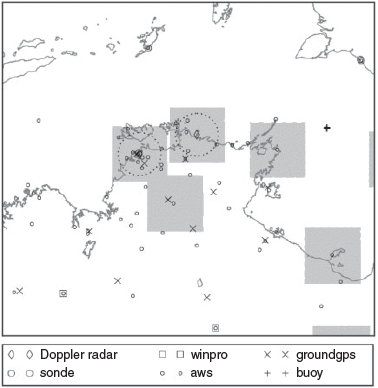
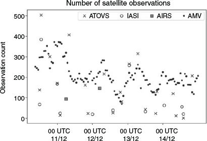
Observations assimilated in these simulations came from automatic weather stations, wind profilers and radiosondes, aircraft, total precipitable water from ground-based GNSS (Global Navigation Satellite System), radial velocity from the Bureau of Meteorology weather radars and AMVs (atmospheric motion vectors, i.e. satellite winds) and sporadic satellite radiances from AIRS, ATOVS and IASI. Observations were extracted from 55 min after the nominal time of each hourly cycle. Additionally, latent heat nudging was applied to the first hour of the model run using half-hourly rainfall accumulations from the national Australian radar composite. Fig. 2 shows spatial coverage of conventional observations (excluding ships and aircraft), Fig. 3 shows temporal availability of satellite observations and Fig. 4 shows the spatial coverage of satellite observations.
|
|

|
The hourly central pressure bogus observations were interpolated from international TC advisories, as is done for the APS3 version of the Bureau of Meteorology’s global model (National Operations Centre 2019). The advisories give a TC location in degrees to one decimal place, and a central pressure in whole hPa. The bogus observations are interpolated hourly between two advisories 6 h apart (Heming 2016). To ensure their assimilation, even if the bogus observations are very different from the model field, the initial Probability of Gross Error, a prior estimate of the probability that an observation might be corrupted and contain no useful information (Lorenc and Hammon 1988), was set to 0 for the bogus observations.
The data assimilation uses the Met Office Observation Processing System (OPS) and variational analysis system (VAR) software for observation processing and assimilation respectively. The hourly 4D-Var (Rawlins et al. 2007) uses an assimilation window spanning between T−30 and T + 30 min for each cycle time (T). It uses static background error covariances as described in Lorenc et al. (2000), but in a model-level formulation arising from swapping the order of vertical and horizontal transform (Wlasak and Cullen 2014). Model-level formulation ensures that length scales characterising the training set are preserved for each model level resulting in the analysis increments appropriately accounting for observational information at both small and large scales. The background error covariances determine how far observation information is spread within the domain, but a spectral formulation is used which does not directly yield the spatial scales.
The model was cold-started from downscaled ACCESS-R initial conditions valid for 0300 UTC 10 December 2018 with data assimilation cycles continuing hourly from 0600 UTC 10 December 2018 to 2300 UTC 17 December 2018. TC Owen entered the domain late on 10 December 2018 and exited late on 14 December 2018. Therefore, the model, while having little time to spin up, was initialised before the TC entered the domain, and the only information from the parent model about the TC came from the lateral boundary conditions.
The hourly data assimilation cycles include short runs of 3 h duration to allow the data assimilation cycling, and longer runs every 3 h of variable duration. The longer runs usually finished at either 1600 UTC (which captures the end of the convective diurnal cycle) for the daytime runs, or at 0900 UTC for the evening runs (to keep the run length shorter). Long run lengths are shown in Table 1. Due to resource constraints, forecast run lengths were kept shorter than might be used operationally. Note that the forecast initiates at 30 min before the specified time and runs for the time shown in Table 1. However, forecast lengths in the results section are referred to from the ‘analysis time’, i.e. the middle of the assimilation window, following normal NWP conventions.

|
The basic differences between the two trials and the operational high-resolution NWP system used for comparison in the results are detailed in Table 2.

|
Cyclone tracks are an important method of cyclone verification. Although there exist some complicated algorithms to estimate the cyclone location, a simple method was chosen for this study. The model forecast tracks are derived by finding the point of lowest pressure in the Gulf, ignoring any low pressures associated with small-scale mesocyclones (which can appear in the bands of convection associated with the vortex) and assuming a central pressure location similar to that of the previous time. Plots of forecast tracks are smoothed by a seven-point (1 h) running mean to aid visibility, as the mean sea level pressure (MSLP) field is output every 10 min. The location and central pressure from the bogus observations are used to represent the ‘truth’.
4 Results
An example of the MSLP and a cross-section of wind is shown in Fig. 5. This demonstrates the effect of assimilating central pressures on the intensity of the cyclone.

|
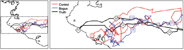
The location of the TC at analysis time (T = 0), essentially the start location of each forecast, was extracted to produce a path of initial or analysis locations. The analysed paths for the two experiments are plotted along with the path from the bogus observations in Fig. 6. The cyclones appear at the eastern boundary at around the right time, influenced by the lateral boundary information from the parent model. Both simulated cyclones lag in travelling westward and do not go as far as the true cyclone. On returning eastward, the simulated cyclones are slower to move, and by 00 UTC 14 December 2018 the cyclones are similarly located. The analysis location for the bogussed cyclone stays closer to the truth from 14 December but does not go as far westward on 12 and 13 December.
|
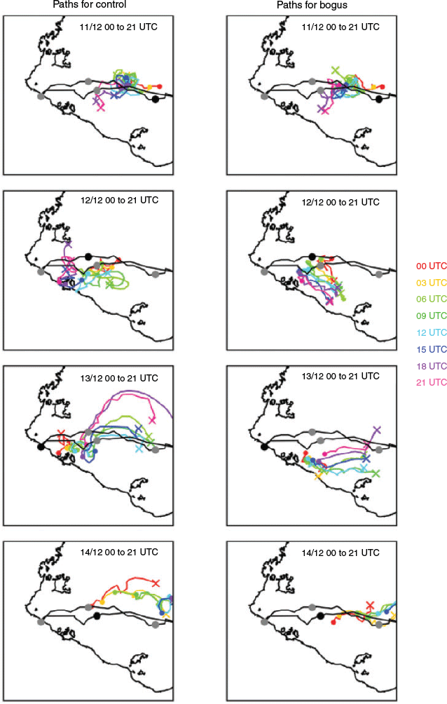
The forecast tracks are shown in Fig 7. The cyclone was late to enter the domain and was slow to move westward initially.
The simulated TCs showed a strong tendency to make landfall too far south-east, which was more pronounced with the bogus run. The control-run cyclone essentially dissipated on landfall, but reformed closer to the true location, while the bogus run stayed south-east, not quite making landfall (Fig. 7b). The bogus-run cyclone location only improved a day later when it shifted northwards, although the turn around to an eastward movement was generally correct. The insufficient westward movement to make landfall suggests the steering flow was too weak in the model.
|
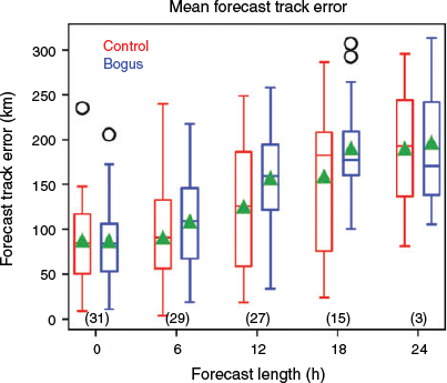
The mean track errors as a function of forecast length were calculated for every forecast base time (eight times per day). Fig. 8 shows a box plot of the track errors. The mean values (horizontal lines) show that the control runs without bogus have smaller errors on average but the spread of the errors is large and the differences are not significant. The large range of errors is likely due to the difficulty in forecasting this cyclone, with weak steering from the lateral boundary conditions. It should be noted that the operational ACCESS models had similar difficulty in forecasting the TC track.
|
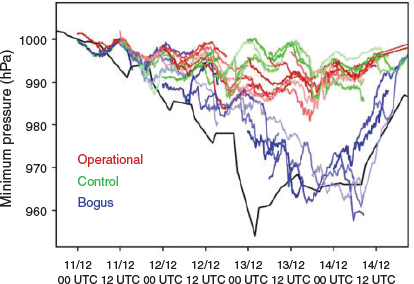
The inclusion of the bogus resulted in a much more realistic central pressure. However, the intensification occurred later and generally finished earlier than was observed (Fig. 9). The timing of the weakening may have been influenced by the proximity of the TC to the eastern boundary. Overall the central pressure was generally 25 hPa higher than observed for the non-bogussed control run at its most intense, while for the bogussed run the central pressure was 10 hPa higher than observed. The cyclone in the non-bogussed control run showed very little deepening, despite the expectation that a mesoscale-resolution cyclone modelling experiment should be capable of producing an intense cyclone. Although the deepening from the inclusion of the bogus is not unexpected, it should be recognised that the result was fairly successful, with only a single observation added to the input of the OPS in each cycle.
|
The tracks and central pressures were also compared against the operational 1.5-km resolution downscaled system (ACCESS-C2), as this is the system to be replaced by the developmental system. This uses a fixed grid with a smaller domain than the developmental system, where the easternmost boundary is 1° further west than the boundary of the variable grid. The TC paths from each base time (ACCESS-C2 is initialised at 00 UTC, 06 UTC, 12 UTC and 18 UTC) are shown in Fig. 10.

|
All simulated cyclones initially have a slow, meandering westward path, turn around sometime around 0000 UTC 13 December 2018, and have a more rapid progression eastward (Fig. 10). All simulations fail to go far enough west, possibly because the parent model, ACCESS-R, also fails to produce the westward movement. In the panels for 14 December 2018 it is also clear the TC does not cleanly exit the domain and some lingering low pressure regions remain near the boundary.
The central pressures for the ACCESS-C2 downscaled runs are shown in comparison to the experiments in Fig. 11. This shows that the ACCESS-C2 central pressures are lower than for the control run. The parent ACCESS-R model does not have a sufficiently deep central pressure, so the initial ACCESS-C2 pressures are not very deep. However, the cyclone may be better represented overall, which allows the cyclone to develop and deepen more during the forecast. Note that a downscaled forecast can require a period of 12–36 h to spin up some features. The bogussed runs are still much better and produce a realistic central pressure.
|
5 Conclusions
The assimilation of bogus observations has been a tactic long used to improve the representation of TCs in global and regional NWP systems, but is not common in convective-scale NWP. This is in part because operational high-resolution simulations using data assimilation over a large tropical region have only become common in recent years, due to the large computing resource requirements, so opportunities have been few.
In this study the effect of using bogus observations is assessed for a TC that entered the ACCESS-DN domain in December 2018. The addition of bogus central pressure observations to the experimental high-resolution, hourly-cycling ACCESS NWP system resulted in marked improvement to the representation of cyclone intensity. The cyclone tracks are roughly accurate in the slower westward movement, turn around and traverse back eastwards along a similar path at a faster rate. However, all simulated paths, whether they are from a downscaled run, or with data assimilation and with or without bogus observations, fail to capture the full westward extent of the path. Indeed, the bogussed experiment had the least westward movement. The depth of the cyclone may have actually made it harder to correct the location of the cyclone, as the amount by which the model fields would need to change becomes larger.
Although the track performance for the experiments both with and without bogus observations was somewhat disappointing, it should be kept in mind that the tracks in a high-resolution nested model are to a large extent dependent on the steering flow imposed by the larger-scale nesting model that provides the boundary conditions. In this case the parent ACCESS-R model forecast tracks suffered similar limitations, suggesting this case has a particularly challenging track to forecast. The ACCESS-R tracks (not shown) followed a similar trajectory to the operational ACCESS-C tracks. Nevertheless, the cyclone with the bogus observations appeared more realistic in terms of cyclone intensity, which should be reassuring for forecasters. This suggests that finding a way to produce bogus observations with short latency would be beneficial for instances when a TC enters one of the ACCESS-City domains, as other available observations may not be sufficient to define the vortex location and structure. However, this conclusion should be confirmed in other cases, especially as the role that the steering flow information from the parent model plays in cyclone development is not quantified.
Conflicts of interest
The authors declare no conflict of interest.
Acknowledgements
This research did not receive any specific funding.
References
Beggs, H., Zhong, A., Warren, G., et al. (2011). RAMSSA - An Operational High-Resolution Multi-Sensor Sea Surface Temperature Analysis over the Australian Region. Aust. Meteorol. Ocean. 61, 1–22.| RAMSSA - An Operational High-Resolution Multi-Sensor Sea Surface Temperature Analysis over the Australian Region.Crossref | GoogleScholarGoogle Scholar |
Bureau National Operations Centre (2016). APS2 Upgrade to the ACCESS-R Numerical Weather Prediction System. Melbourne, Australia. Available at: http://www.bom.gov.au/australia/charts/bulletins/apob107-external.pdf.
Bureau National Operations Centre (2017). APS2 Upgrade to the ACCESS-TC Numerical Weather Prediction System. Melbourne, Australia. Available at: http://www.bom.gov.au/australia/charts/bulletins/BNOC_Operations_Bulletin_112.pdf.
Bureau National Operations Centre (2018). APS2 upgrade of the ACCESS-C Numerical Weather Prediction system. Melbourne, Australia. Available at: http://www.bom.gov.au/australia/charts/bulletins/BNOC_Operations_Bulletin_114.pdf.
Bush, M., Allen, T., Bain, C., et al. (2020). The first Met Office Unified Model/JULES Regional Atmosphere and Land configuration, RAL1. Geosci. Model Dev. 13, 1999–2029.
| The first Met Office Unified Model/JULES Regional Atmosphere and Land configuration, RAL1.Crossref | GoogleScholarGoogle Scholar |
Davidson, N. E., Xiao, Y., Ma, Y., et al. (2014). ACCESS-TC: Vortex Specification, 4DVAR Initialization, Verification, and Structure Diagnostics. Mon. Wea. Rev. 142, 1265–1289.
| ACCESS-TC: Vortex Specification, 4DVAR Initialization, Verification, and Structure Diagnostics.Crossref | GoogleScholarGoogle Scholar |
Heming, J. T. (2016). Met Office Unified Model Tropical Cyclone Performance Following Major Changes to the Initialization Scheme and a Model Upgrade. Wea. Forecasting 31, 1433–1449.
| Met Office Unified Model Tropical Cyclone Performance Following Major Changes to the Initialization Scheme and a Model Upgrade.Crossref | GoogleScholarGoogle Scholar |
Lorenc, A. C., Ballard, S. P., Bell, R. S., et al. (2000). The Met. Office global three-dimensional variational data assimilation scheme. Quart. J. Roy. Meteor. Soc. 126, 2991–3012.
| The Met. Office global three-dimensional variational data assimilation scheme.Crossref | GoogleScholarGoogle Scholar |
Lorenc, A. C., and Hammon, O. (1988). Objective quality control of observations using Bayesian methods: theory, and a practical implementation. Quart. J. Roy. Meteor. Soc. 114, 205–239.
| Objective quality control of observations using Bayesian methods: theory, and a practical implementation.Crossref | GoogleScholarGoogle Scholar |
National Operations Centre (2019). APS3 upgrade of the ACCESS-G/GE Numerical Weather Prediction system. Melbourne, Australia. Available at: http://www.bom.gov.au/australia/charts/bulletins/opsbull_G3GE3_external_v3.pdf.
National Operations Centre (2020). APS3 upgrade of the ACCESS-TC Numerical Weather Prediction system. Melbourne, Australia. Available at: http://www.bom.gov.au/australia/charts/bulletins/opsbull_ACCESS_TC3_External.pdf.
Puri, K. A., Dietachmayer, G., Steinle, P. J., et al. (2013). Implementation of the initial ACCESS numerical weather prediction system. Aust. Meteorol. Ocean. 63, 265–284.
| Implementation of the initial ACCESS numerical weather prediction system.Crossref | GoogleScholarGoogle Scholar |
Rawlins, F., Ballard, S. P., Bovis, K. J., et al. (2007). The Met Office global four-dimensional variational data assimilation scheme. Quart. J. Roy. Meteor. Soc. 133, 347–362.
| The Met Office global four-dimensional variational data assimilation scheme.Crossref | GoogleScholarGoogle Scholar |
Wlasak, M. A., and Cullen, M. J. P. (2014). Modelling static 3-D spatial background error covariances – the effect of vertical and horizontal transform order. Adv. Sci. Res. 11, 63–67.
| Modelling static 3-D spatial background error covariances – the effect of vertical and horizontal transform order.Crossref | GoogleScholarGoogle Scholar |