The Australian wave forecast system with statistical wind correction
Stefan Zieger A *
A *
A
Handling Editor: Anthony Rea
Abstract
The Bureau of Meteorology (the Bureau) has an important role in providing marine services around Australia and its oceans. These services strongly depend on guidance from numerical wave models, which depend on numerical weather and ocean prediction systems. The Bureau has upgraded its collective suite of all numerical models to the Australian Parallel Suite (APS) 4. The APS systems have vastly improved their skill because of increased resolution, enhanced data assimilation (including increasing numbers and types of observations) and improvements in physical parameterisations. This paper verifies the skill of the numerical weather prediction model and the underlying wave model using observations from satellite systems and wave buoys. The characteristics of the surface winds led to the development of a statistical wind correction (i.e. bias correction) that superseded the flux-scaling applied in the APS3 version. Comparisons to the legacy wave model and the European Centre for Medium-Range Weather Forecast reanalysis ERA5 indicate that the Bureau’s global wave forecast system outperforms both across a few metrics. Satellite altimetry verification shows an improvement in root-mean-square error, variability, probability of exceedance and probability density function. Wave buoy verification around Australia agrees with the skill assessment from satellite altimeters. Looking at the root-mean-square error of significant wave height, there is an estimated mean error of 0.29 m for altimeter observations and across 84 wave buoy locations.
Keywords: AUSWAVE, ERA5, ST6, wave forecasting, wave model, wave verification, WAVEWATCH III, wind bias correction.
1.Introduction
The Bureau of Meteorology (hereafter the Bureau) provides marine services for Australia and the surrounding oceans. Services assist marine operators and vessels in many ways, with the most critical one supporting safe operations without fatalities at sea. Marine forecasts can avoid environmental disasters and assist in search and rescue operations. Forecast services come from numerical wave models. Numerical weather prediction (NWP) systems drive these wave models, and the Australian Parallel Suite (APS) is the collective suite of all numerical models. The third generation of the Bureau’s model suites, APS3, included Australia’s first global weather ensemble system (National Operations Centre 2020). The Bureau upgraded the suite recently to the next generation, APS4.
The Australian Wave Model (AUSWAVE) is the Bureau’s implementation of the third-generation wave model WAVEWATCH III (WW3) (ver. 6.07, see https://github.com/noaa-emc/ww3; The WAVEWATCH Dev. Group 2019). The global version AUSWAVE-G features a multiple-resolution spherical-multiple cell (SMC) grid at 12-km resolution, with refinement around islands and shelves with water depth of less than 300 m at ~6 km (Zieger and Greenslade 2021). Incorporating surface fields from APS4, namely the global numerical weather prediction system’s wind components, Australian Community Climate and Earth-System Simulator (ACCESS) and the Ocean Model, Analysis and Prediction System (OceanMAPS 4.1i) surface current components, requires reconfiguring the wave model. OceanMAPS is the Bureau’s data-assimilating ocean prediction system (Brassington et al. 2007; National Operations Centre 2024). The real-time sea ice analysis at 1/12° resolution of the National Centre for Environmental Prediction (NCEP)–National Oceanic and Atmospheric Administration (NOAA) is used to represent the effect of varying fetch due to sea ice coverage.
Dynamical wave models simulate the variance density spectrum of surface gravity waves, with the primary source terms behind wave growth being the wind input, resonant four-wave interaction and dissipation. Third-generation means the wave model explicitly accounts for the four-wave resonant term (Hasselmann et al. 1985). Historically, the wind input term relied on tuning to compensate for biases in the atmospheric surface fields, and it can very well change when switching the forcing product (e.g. Tolman 1998; Tolman et al. 2002; Oladejo et al. 2025). At the time of writing, the most common publicly available atmospheric reanalysis products are from the European Centre for Medium-Range Weather Forecast (ECMWF), ECMWF Reanalysis (5th gen., ERA5), and from NOAA-NCEP, Climate Forecast System 2 (CFS2) (Saha et al. 2014). The characteristics of reanalyses differ when looking at the tail of the wind speed distribution (e.g. Alday et al. 2021; Liu et al. 2021; Gandoin and Garza 2024).
Compensating for wind speed characteristics in the wave model depends on the type of wind input term. In a model with the Miles–Janssen-type input, like WAM Cycle 4 (Janssen 1991; Komen et al. 1994), the fluxes can be adjusted as a whole through the so-called βmax parameter. By contrast, the observation-based input term in WW3 uses a scaling parameter to adjust the drag coefficient FLX4 (Hwang 2011; The WAVEWATCH Dev. Group 2019). The fundamental difference is that the Miles–Janssen-type input takes a linear form and overcompensates the drag coefficient from and above gale-force wind speed (Durrant et al. 2013). On the other hand, the Hwang drag parameterisation accounts for saturation and a decrease in magnitude for extreme winds. Valiente et al. (2021) and Meucci et al. (2023) provide illustrative examples highlighting differences in these two parameterisations. Wave modelling frequently applies the Miles–Janssen-type input, and thus, there is a flurry of values for βmax in the literature. Cited values for βmax include 1.2 (Bidlot et al. 2005), 1.25 (Stopa et al. 2016), 1.28 (Breivik et al. 2022), 1.36 (Oladejo et al. 2025), 1.39 (Valiente et al. 2023), 1.52 (Ardhuin et al. 2010) and 1.75 (Alday et al. 2021).
This study aims to demonstrate that wave model skill depends on the characteristics of the surface wind fields and that bias correction is a valid technique for calibrating a wave model. A significant challenge in operational global wave modelling was the separation of internal errors (wave model) and external errors due to wind forcing. Rogers et al. (2005) concluded that for wave model predictability, the wind speed bias at moderate to high wind speeds is more important than the overall bias. Tolman et al. (2013) highlighted the need to improve the operational wave model due to known biases in some cases that yield novel physics and numerical schemes in WW3 (Tolman and the WAVEWATCH Dev. Group 2014). Wave model physics should accurately predict surface waves from open ocean to enclosed seas, from calm to extreme conditions (e.g. tropical cyclones).
This paper is organised as follows. Section 2 outlines the Bureau’s numerical models and includes global verification metrics based on satellite observations. Section 3 assesses forecast errors and verification across wave buoys. Section 4 contains a discussion, followed by a conclusion in Section 5. Appendices include a list of verification metrics as well as a list of frequently used acronyms.
2.Australian Parallel Suite (APS)
2.1. Atmospheric model
The UK Met Offices’ unified model is the basis for the APS weather model. The fourth upgrade (APS4) contains the UK Met Offices’ Parallel Suite 45 code, designed to run with a dynamic ocean model. However, the current implementation uses static sea surface temperature fields. Coupling to a dynamic ocean is planned at a later stage.
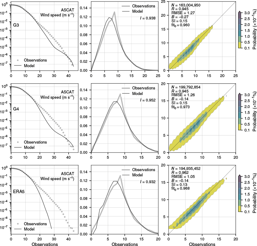
Fig. 1 and Table 1 show verification metrics for various weather models relative to marine advanced scatterometer (ASCAT) winds. A couple of things stand out. First, APS4 shows a reduced wind bias relative to APS3, from −0.27 to −0.12 m s−1. Second, the root-mean-square error (RMSE; ) in wind speed improved from 1.27 to 1.26 m s−1. Third, there is a better representation of the probability density function (central panel) in APS4. However, the probability of exceedance P(X > x) shows lower skill in APS4, meaning that high wind speeds in the range of 18–35 m s−1 are less accurate. Interestingly, APS3 is slightly better for P(X > x) than APS4. For comparison, Durrant et al. (2013) found a negative bias (B; ) of −0.52 m s−1 with RMSE of 1.57 m s−1 in the APS1 wind field and applied bias correction. The NWP reanalysis, for example, ERA5 (Hersbach et al. 2020) is known for biases at high wind speed; hence, statistical correction for extreme winds is valid. The bottom-left panel in Fig. 1 shows that the probability of exceedance of ERA5 surface wind speed is under-predicted, starting at ~17 m s−1, also reflected in a lower value for slope and a lower score in histogram fit (I; ; Swain and Ballard 2002) (see legend in the central panel). Nonetheless, the ERA5 reanalysis features the best skill regarding RMSE, scatter index (SI; Cardone et al. 1996; s.d.(m – o) ÷ mean(o)) and Pearson’s correlation coefficient (R). It is therefore considered the best product in the world.
Satellite verification statistics for marine winds from ACCESS-G3 (top), ACCESS-G4 (centre) and ERA5 (bottom). Statistics were averaged globally from July 2023 to August 2024. Panels show the probability of exceedance (left), probability density function and scatter density (right). Statistics in the legend are the number of observations (N), Pearson’s correlation coefficient (R), root-mean-square error (RMSE), bias (B), scatter index (SI), least squares slope forced through the origin (fit0) and histogram fit (I).
| Label | R | RMSE (m s−1) | MAE (m s−1) | B (m s−1) | SI | fit0 | s.d.(O) (m s−1) | s.d.(M) (m s−1) | I | |
|---|---|---|---|---|---|---|---|---|---|---|
| G3 | 0.945 | 1.27 | 0.91 | −0.27 | 0.15 | 0.96 | 3.77 | 3.72 | 0.938 | |
| G4 | 0.945 | 1.26 | 0.89 | −0.14 | 0.15 | 0.97 | 3.79 | 3.72 | 0.952 | |
| ERA5 | 0.962 | 1.05 | 0.73 | −0.14 | 0.13 | 0.97 | 3.80 | 3.52 | 0.932 |
Statistics were averaged globally from July 2023 to August 2024. Statistics are Pearson’s correlation coefficient (R), root-mean-square error (RMSE), mean absolute error (MAE), bias (B), scatter index (SI), least squares slope forced through the origin (fit0), standard deviation of model (s.d.(M)) and standard deviation of observations (s.d.(O)), and histogram fit (I).
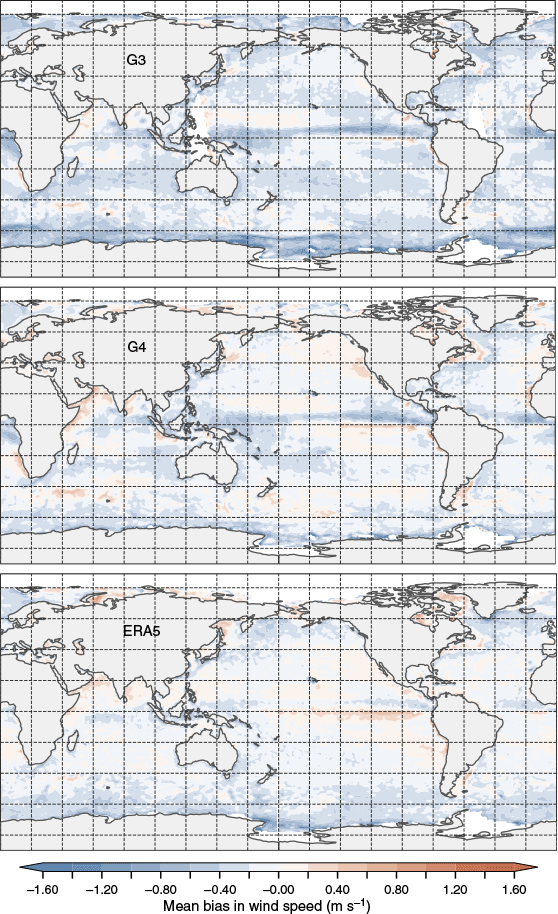
Fig. 2 shows the spatial distribution of mean wind bias from July 2023 to August 2024. It confirms the reduction in wind speed bias with fewer blueish regions visible in APS4 overall than in APS3. The most noticeable improvements are along the Antarctic ice edge, the equatorial Pacific and the eastern Indian Ocean. The western Indian Ocean remains biased low. Spatial patterns in ERA5 reanalysis bias are like those in ASP4, perhaps except for the Southern Ocean, where more frequent underestimation of surface winds occurs.
Spatial mean wind speed bias from (top to bottom) ACCESS-G3, ACCESS-G4 and ERA5. Observations refer to ASCAT satellite data from July 2023 to August 2024.
The negative bias in wind speed originates from a prescribed static wave-boundary layer. The NWP operates as a standalone model. Two-way coupling can reduce biases at high wind speeds and decrease the scatter (Wiese et al. 2020). Janssen and Bidlot (2018) illustrated the importance of two-way coupling and stress, stating that the principal component is the transfer of momentum and energy to the surface. Breivik et al. (2022) showed that reducing the Charnock parameters at high wind speeds can increase wind speed in the wave-boundary layer.
2.2. Wave model
AUSWAVE-G is based on a 12-km multiple-resolution SMC grid, with refinement around sub-grid scales features and shelves at ~6 km and features the observation-based wind input and dissipation terms (Zieger and Greenslade 2021). The legacy AUSWAVE-G APS3 uses the GEBCO 2020 (GEBCO Bathymetric Compilation Group 2020) gridded bathymetry data. Bathymetric depths were evaluated against measured depths derived from wave buoy deployments around the Australian coastline. The APS4 upgrade did not change the wave model grid and underlying bathymetry.
Surface gravity waves grow due to surface winds. Wave equilibrium assumes the dominant terms (i.e. wind input, resonant wave–wave interaction and wave breaking) on the right-hand side in balance and the left-hand side of the governing equation to be zero at first order (Thomson et al. 2013). Equilibrium wave theory shows that significant wave height Hs scales with wind speed (Janssen 1998). This means that the error in the wind field is related to the error in the wave field. A detailed skill assessment of the global wind field is essential for the predictability of the wave field. Satellite verification yields an error of 1.26 m s−1 in the surface wind field (global averages), which would result in an error of 0.41 m in significant wave height. The negative bias in the ACCESS wind field (APS1) yields a negative bias in the wave field with a Hs bias of −0.22 m and RMSE of 0.49 m (Durrant et al. 2013). Durrant and co-authors concluded that the bias in Hs is highly sensitive to the bias in U10, overall and in spatial variation.
The global wave model AUSWAVE-G APS3 increased the skill on average by 13% compared to the previous version (Zieger and Greenslade 2021). The improvement comes from increasing the flux to the waves by 5% to compensate for inherent biases in surface wind speed. Setting the FLX4 namelist parameter CDFAC to 1.05 increases the fluxes from the atmosphere to the waves by 5%. Initial trials of the legacy AUSWAVE-G3 model with ACCESS-G4 surface winds were unsatisfactory. They resulted in a large overprediction of the wave field with less skilful bulk scatter statistics (i.e. bias, RMSE, SI and R), as shown in Table 2. Scaling the drag coefficient would change the momentum flux across the entire range of surface winds, leading to an overestimate in the low range. The wave model then integrates these overestimates, producing less skilful wave predictions. As a result, to compensate for biases in the wind field, a bias correction will be adopted.
| Label | CDFAC | w1 | w2 | R | RMSE (m) | B (m) | SI | fit0 | |
|---|---|---|---|---|---|---|---|---|---|
| G3 | 1.05 | n/a | n/a | 0.974 | 0.29 | −0.01 | 0.12 | 0.99 | |
| G3 with APS4 winds | 1.05 | n/a | n/a | 0.966 | 0.36 | 0.07 | 0.14 | 1.01 | |
| G4 | 1.00 | 18.0 | 0.40 | 0.975 | 0.29 | 0.01 | 0.11 | 0.99 | |
| ERA5 | n/a | n/a | n/a | 0.974 | 0.31 | −0.06 | 0.12 | 0.96 |
G3 refers to the operation wave model. G4 is the new wave model configuration for APS4 model fields. ERA5 refers to ECMWF reanalysis for reference. CDFAC is the non-dimensional scaling parameter for drag parameterisation FLX4. Pearson’s correlation coefficient (R); root-mean-square error (RMSE), bias (B), scatter index (SI) and least squares slope forced through the origin (fit0).
Verification of concatenated 12-h forecasts of ACCESS-G4 reveals a slight bias in wind speed (see Fig. 1). A close look at the probability of exceedance plot (left panel) indicates that the surface winds are in excellent agreement to ~15 m s−1. An adjustment of only a fraction of the winds is needed. To do so, we apply a threshold-based bias correction to target the underprediction of extreme surface winds with wind magnitudes that exceed the threshold w1 are scaled with w2 as defined in Eqn 1.
Table 2 lists configurations with variations in wind speed correction and the resulting altimeter verification for the wave model simulation. Since the surface wind speed skill is remarkably close between the APS3 and APS4 versions of the NWP model, one would expect a similar skill between the AUSWAVE versions. The change in wind speed bias from −0.27 to −0.14 m s−1 will overestimate the sea state everywhere with a mean bias of 0.07 m in significant wave height and 2% increase in SI, as listed in Table 2. The threshold-based approach applied here can alleviate this overestimate. A closer look at the metrics in Table 2 reveals that the bias correction improves the legacy model G3 in SI, R and bias. Fig. 3 shows that the G4 wave model matches the probability density function of the observations and represents extreme wave heights exceptionally well to the point that it can beat ERA5 in skill. One can conclude that open ocean fields of Hs are verified well by altimeter observations.
Satellite verification for significant wave height. Statistics are for the AUSWAVE-G3 operational model (top), the configuration for AUSWAVE-G4 (centre) and ERA5 (bottom). Statistics are averaged between 55°N and 55°S from 1 August 2023 to 1 January 2023 and 22 February to 1 August 2024. Panels show the probability of exceedance (left), probability density function and scatter density (right). Statistics in legend are the number of observations (N), Pearson’s correlation coefficient (R), root-mean-square error (RMSE), bias (B), scatter index (SI), least squares slope forced through the origin (fit0) and histogram fit (I).
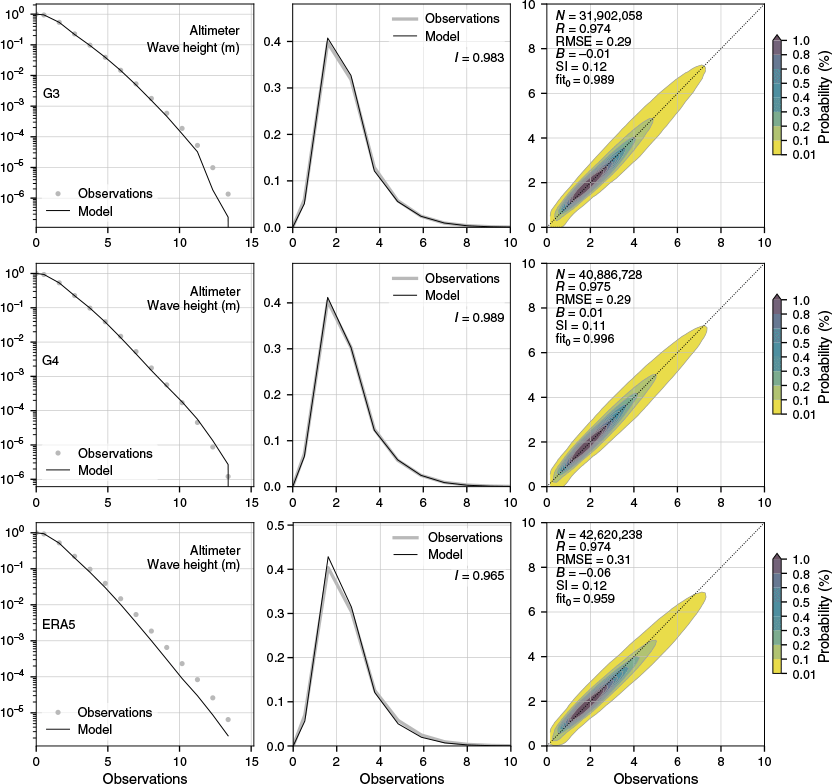
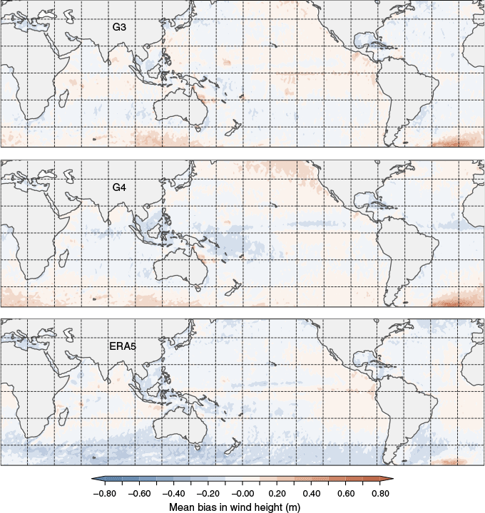
Fig. 4 shows the spatial distribution of mean Hs observed by altimeters. ASP3 and APS4 are similar in bias patterns. At high latitudes, the APS4 bias (middle panel) is slightly larger than that of APS3, which may result from the somewhat more energetic surface winds (see Fig. 2). By contrast, these regions are prominent for long-period swells, indicating a lack of understanding of swell dissipation. The most noticeable difference in ERA5 reanalysis is a more prominent negative bias in Hs in the Southern Ocean, North Pacific and North Atlantic. The G4 model features a more negative bias in the west-central equatorial Pacific, while a positive bias persists east of Drake Passage in the South Atlantic.
Spatial mean bias in significant wave height. Panels show from top to bottom: AUSWAVE-G3, AUSWAVE-G4 and ERA5. Observations refer to altimeter data with statistics averaged between 55°N and 55°S from 1 August 2023 to 1 January 2023 and 22 February to 1 August 2024.
The third-generation spectral wave model WW3 explicitly contains source terms representing swell decay and negative input. The wave model in the ERA5 reanalysis does not contain an explicit swell decay term. Instead, the level of white-capping dissipation was retuned to mimic the slow attenuation of long-period swell (Hersbach et al. 2020). The negative input in WW3 represents non-breaking dissipation due to turbulence in the atmosphere–wave boundary layer. Although the swell decay rate has been observed in field experiments, one cannot distinguish background interaction on either side of the sea surface, i.e. in the air or water (Young et al. 2013). Pathirana et al. (2023) found that swell waves are attenuated too strongly for swells propagating long distances and recommended a lower value for negative wind input in observation-based wave physics (ST6). Zieger et al. (2015) and later Liu et al. (2019) fully describe the ST6 physics package. An earlier version of the configuration with a negative input of 5% and a constant swell decay coefficient is selected (Zieger et al. 2015), consistent with the conclusion of Pathirana et al. (2023). In addition, the background turbulence swell dissipation rate is constant b1 = 0.22 × 10⁻³. The rest of the model configuration follows the configuration described in Zieger and Greenslade (2021).
3.Extended verification
3.1. Forecast verification
Results presented in Section 2 demonstrated the skill of the new model configuration compared to the legacy operational wave model and ERA5 reanalysis for open ocean and deep-water wave conditions from altimeter observations. The wave hindcasts were forced with concatenated 12-h NWP forecasts, including analysis fields and short-range forecasts, to minimise the accumulation of forecast errors. Hindcasts are free simulations with no explicit use of data assimilation. Under the assumption that forecast errors grow with lead time, these short-range forecasts will have the most negligible errors associated with them.
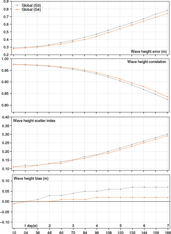
We cycled the model every 12 h to assess the forecast skill and produced 7-day forecasts for March–November 2024 to generate a database for forecast verification. Fig. 5 shows the skill for Hs as a function of forecast lead time and demonstrates that the proposed G4 configuration outperforms or matches the legacy global system (G3) entirely. The RMSE (top panel in Fig. 5) does not change significantly over the first +2 to +3 days and then grows at a higher rate during days 3–7. Interestingly, the forecast error is persistently lower than the error of the legacy model (G3) and accumulates at a lower rate with forecast lead time. A similar pattern is evident when looking at R in significant wave height (second panel from the top in Fig. 5). R is close to the legacy system up to the 3-day forecast range. Beyond 3 days, the new model features less R loss. AUSWAVE-G3 showed an increase in bias with a lead time of up to 5 days (bottom panel in Fig. 5). The G4 model configuration reduced the model bias with lead time.
Model skill for significant wave height plotted as a function of forecast time (hours, horizontal axis). Panels show verification metrics (top to bottom): root-mean-square error, Pearson’s correlation (R), scatter index (SI) and bias (B). Line colours indicate different models, as indicated in the legend.
Zieger and Greenslade (2021) showed that the forecast errors in APS3 surface winds grow linearly across the full forecast range. The wave model takes ~3 days in lead time to accumulate errors in new wind-sea from the NWP model and propagate these uncertainties across the sea as swell. Swell waves differ from local wind-sea and originate from remote storms much earlier. The data assimilation in NWP models ensures high precision of storm location, allowing for accurate swell propagation at short time scales away from the storm centres (Komen et al. 1994). Swell waves are lower in magnitude than wind waves; therefore, errors associated with wind-sea waves are more significant than those for swells. For example, Southern Ocean swells dominate Australia’s North-West Shelf, and wave buoy verification shows smaller RMSE and mean absolute error (MAE; ) than all of Australia (Table 3). Pathirana et al. (2023) quantified swell presence in over 75% of the oceans, which can explain the lag in lead time in forecast error. The rate of error accumulation is higher in the NWP model than in the wave model.
| Label | N | R | RMSE (m) | MAE (m) | B (m) | SI | fit0 | s.d.(O) (m) | s.d.(M) (m) | I | |
|---|---|---|---|---|---|---|---|---|---|---|---|
| G3 | 583,076 | 0.963 | 0.30 | 0.22 | 0.05 | 0.19 | 1.00 | 1.10 | 1.06 | 0.953 | |
| G4 | 593,935 | 0.965 | 0.29 | 0.21 | 0.06 | 0.19 | 1.00 | 1.10 | 1.06 | 0.951 | |
| ERA5 | 512,289 | 0.936 | 0.40 | 0.28 | 0.05 | 0.25 | 0.97 | 1.14 | 1.03 | 0.948 | |
| NOAA wave buoys | |||||||||||
| G4 | 154,860 | 0.968 | 0.30 | 0.22 | 0.08 | 0.12 | 1.01 | 1.15 | 1.08 | 0.959 | |
| ERA5 | 154,860 | 0.962 | 0.34 | 0.24 | −0.07 | 0.13 | 0.95 | 1.15 | 0.99 | 0.952 | |
| Australian North-West Shelf wave buoys | |||||||||||
| G4 | 96,153 | 0.918 | 0.28 | 0.16 | 0.02 | 0.33 | 0.92 | 0.70 | 0.58 | 0.965 | |
| ERA5 | 96,148 | 0.886 | 0.34 | 0.21 | 0.09 | 0.38 | 0.95 | 0.70 | 0.56 | 0.931 | |
| NOAA wave buoy 46070 (south Bering Sea) | |||||||||||
| G4 | 13,169 | 0.979 | 0.33 | 0.23 | −0.01 | 0.12 | 0.97 | 1.54 | 1.40 | 0.954 | |
| ERA5 | 13,169 | 0.979 | 0.39 | 0.26 | −0.15 | 0.13 | 0.92 | 1.54 | 1.33 | 0.934 | |
| Southern Ocean Flux Station | |||||||||||
| G4 | 4641 | 0.936 | 0.53 | 0.36 | 0.01 | 0.13 | 0.99 | 1.51 | 1.39 | 0.967 | |
| ERA5 | 4641 | 0.930 | 0.61 | 0.43 | −0.23 | 0.14 | 0.93 | 1.51 | 1.30 | 0.929 | |
Statistics are averaged from 1 August 2023 to 1 January 2023 and 22 February to 1 August 2024. Metrics include number of observations (N), Pearson’s correlation coefficient (R), root-mean-square error (RMSE), mean absolute error (MAE), bias (B), scatter index (SI), least squares slope forced through the origin (fit0), standard deviation of model (s.d.(M)) and standard deviation of observations (s.d.(O)), and histogram fit (I). Rows indicate averages over different sets and individual sites (see text for details).
3.2. Site-based verification
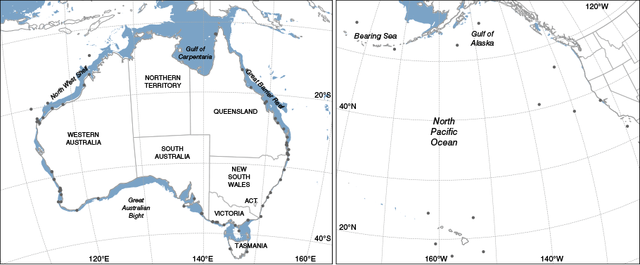
Altimeter verification presented in previous sections demonstrated skill improvements when applying bias correction in the new model configuration for open-ocean sea states. However, most users of operational wave forecasts are interested in the coast, and most wave buoys around Australia are located near the coast, as shown in Fig. 6. The Southern Ocean Flux Station, SOFS (Schulz et al. 2012), is omitted in Fig. 6 due to its location ~640 km south-south-west of Tasmania. We included US wave buoys from the North Pacific to verify the model skill in the open ocean. Open ocean refers to sites with depths greater than half the mean wavelength and a few kilometres distant from the coast. In deep-water locations, the wave field is unaffected by coastline geometry and the processes associated with limited depth and shallow water.
Location of in situ wave buoys used for verification. There are 69 sites around Australia (left panel) and 14 in the North Pacific (right panel). Solid blue shading indicates the width of the continental shelf (i.e. areas of less than 75-m depth).
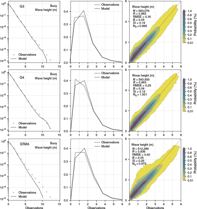
Wave hindcast skill across all in situ wave buoys listed in Table 3 and Fig. 7. The results are close to identical for G3 and G4. A closer look at the metrics in Table 3 shows almost no difference, and the results agree with the altimeter verification presented earlier. A global RMSE of 0.29 m is a slight improvement from that of G3 for the same period. Compared to G3, G4 improves in the tail of the probability of exceedance – a small but noteworthy improvement. The ERA5 reanalysis compares well in terms of the shape of the probability density function, as shown in the second column panels in Fig. 7. The ERA5 shows an increase in scatter in Hs in the range up to ~2.5 m. The frequency of extreme Hs appears to be underrepresented in ERA5 and scatter density plots indicate that the bulk of scatter above 2.5 m falls below the line of best fit with a regression coefficient of the least squares slope forced through the origin (fit0) of 0.972. Table 3 also indicates that the skill in ERA5 wave reanalysis is not far behind that of the G4 model for wave buoys located in the North Pacific and the North-West Shelf of Australia.
Wave buoy verification for significant wave height. Statistics are for the AUSWAVE-G3 operational model (top), the configuration for AUSWAVE-G4 (centre) and ERA5 (bottom). Statistics are averaged between 55°N and 55°S from 1 August 2023 to 1 January 2023 and 22 February to 1 August 2024. Panels show the probability of exceedance (left), probability density function and scatter density (right). Statistics in legend are the number of observations (N), Pearson’s correlation coefficient (R), root-mean-square error (RMSE), bias (B), scatter index (SI) and least squares slope forced through the origin (fit0).
One interesting feature in Table 3 is that the ERA5 reanalysis features a negative bias at high latitudes, i.e. North Pacific wave buoys. By contrast, the opposite is true at low latitudes, i.e. Australian wave buoys. The bottom panel in Fig. 4 confirms this feature and shows the spatial distribution of biases. One can only speculate on the source of these biases. The spatial winds bias shown in Fig. 2 does not support such a trend.
The wave model (AUSWAVE) and wave reanalysis have different resolutions. The spatial resolution of AUSWAVE is 0.125°, with refinements of 0.0625° around islands and continental shelves. The ERA5 wave reanalysis fields are archived at 0.50°, whereas the wave model resolution is 0.36° (Hersbach et al. 2020). Bulk statistics in Table 3 omit wave buoy locations that fell within the land mask of the reanalysis and exclude locations mapped too far offshore. Offshore locations tend to increase the variability, i.e. standard deviation, and introduce a representation bias in the model. As a result, there is a divergence in the number of data points used in buoy verification.
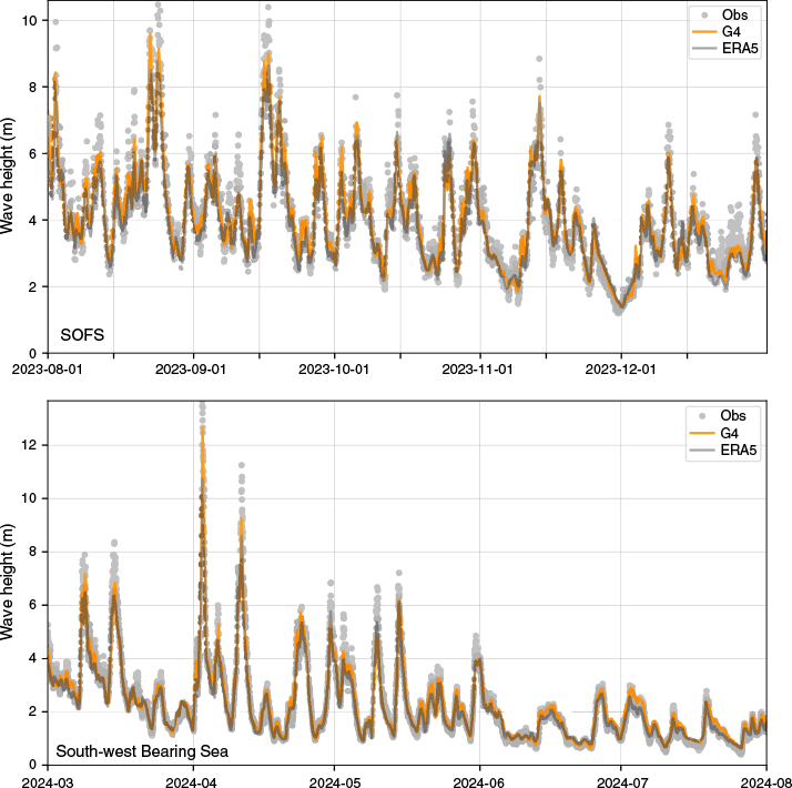
Bulk metrics in Table 3, such as RMSE and R, do not adequately reflect the model’s performance at the distribution’s tail, as shown in the probability of exceedance in Fig. 7. For illustrative purposes, we plotted wave buoy time series for two stations with frequent extreme waves. Figures 8 and 9 show the time series of Hs and wave period for SOFS (Schulz et al. 2012), located south-south-west of Tasmania (Southern Hemisphere), and NOAA wave buoy 46070, located in the south Bering Sea (Northern Hemisphere). The agreement between the models and observations is remarkable for Hs. The SOFS observations show more scatter than the NOAA buoy. The wave model skill at the SOFS location is the lowest in the verification, highlighting the challenges in wave modelling in the Southern Hemisphere with an ocean subject to infinite fetch. The onset of peaks in the time series matches very well for both models, resulting in a R greater than 0.93. Nonetheless, the peaks in Hs are higher in the G4 model. Surprisingly, this is not just the case for Hs above 10 m, as indicated in the probability of exceedance plots. A similar pattern for Hs exists below 10 m, where G4 peaks exceed those of ERA5. Local minima in the time series match between models, concluding that the G4 model has greater variability in Hs than the ERA5 wave reanalysis, and Table 3 shows that the standard deviation of G4 is persistently above the standard deviation of ERA5.
Time series of significant wave height (Hs) observed by wave buoys and predicted by AUSWAVE-G4 and ERA5. The panel shows (from top) the Southern Ocean Flux Station (141.3°E 47.2°S) and NOAA wave buoy 46070 (south-west Bering Sea; 175.3°W 55.1°N).
Time series of wave period observed by wave buoys and predicted by AUSWAVE-G4 and ERA5. The panel shows the mean zero-crossing periods (Tz) at the Southern Ocean Flux Station (141.3°E 47.2°S) and the peak wave periods (Tp) at NOAA wave buoy 46070 (south-west Bering Sea; 175.3°W 55.1°N).
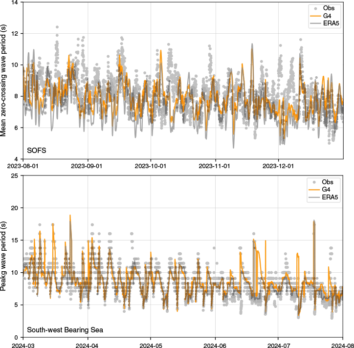
Verification for the wave periods is more challenging than for significant wave height. Owing to data processing, there is inherently more scattering in the buoy observations. Fig. 9 shows an increase in scatter in the observations for zero-crossing and peak wave periods compared to Hs (Fig. 8). There is better agreement between the models than between the model and buoy observations. An increase in scatter yields a reduction in the R between the model and observations for the wave periods, with values of ~0.7–0.8. The similarity within the wave models is unsurprising since the models share a standard spectral resolution with frequencies logarithmically spaced, which differs to the frequency discretisation used in buoy data processing. Another shared aspect is that the wave models use the same methodology to calculate the resonant four-wave interaction. This method is critical for the down-shift of the peak of the wave spectrum, effectively allowing the wave field to outrun the storm and transition from wind waves to swell (Hasselmann 1960).
4.Discussion
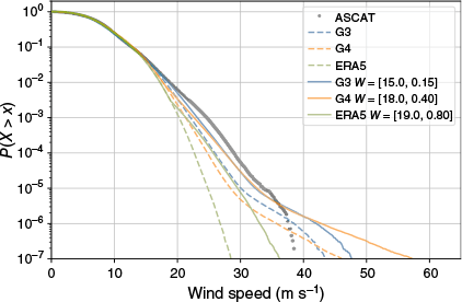
The bias correction presented here is a linear method to enhance the tail of the wind speed distribution. The value for scaling w2 depends on the choice of threshold w1, and a lower threshold requires a lower value for scaling. Fig. 10 illustrates the effect of different bias correction coefficients applied to NWP models and reanalysis. A bias correction for APS3 and APS4 surface winds is in close agreement, up to 40 m s−1. The coefficients differ, however, with G3 using a lower threshold and scaling coefficient compared to G4. For ERA5, potential bias correction would require higher coefficients than that of G4, as indicated in the figure legend. Alday et al. (2021), for example, used values of w1 = 21.0 m s−1 and w2 = 1.05 to compensate for the high wind speed bias in ERA5 for a WW3 hindcast with a Miles–Jansen-type input and a βmax = 1.75 (Ardhuin et al. 2010). Looking at bulk verification metrics, the bias correction from Fig. 10 merely affects the skill, and the scores listed in Table 4 are very close to those for the uncorrected winds shown in Table 1 and Fig. 1. In this context, ‘merely affects skill’ refers to the improvement in RMSE stemming from the bias correction of 0.02 m s−1 for APS4 and 0.01 m s−1 for ERA5. The R increases by 0.01 for APS4 and ERA5 when bias correction is applied, and the skill is unchanged when looking at the SI. However, it has a profound effect when applied to the wave model and can reduce the RMSE, bias and SI in Hs significantly as shown in Table 2.
Probability of exceedance P(X > x) of surface wind speed. NWP and the reanalysis are separated by colour and plotted with dashed lines. Solid lines mark the bias correction with correction coefficients W = [w1, w2] listed in the legend. Verification data cover the period from January 2023 to August 2024.
| Label | w1 | w2 | R | RMSE (m s−1) | MAE (m s−1) | B (m s−1) | SI | fit0 | s.d.(O) (m s−1) | s.d.(M) (m s−1) | I | |
|---|---|---|---|---|---|---|---|---|---|---|---|---|
| G3 with BC | 15.0 | 0.15 | 0.945 | 1.27 | 0.91 | −0.26 | 0.15 | 0.96 | 3.77 | 3.74 | 0.938 | |
| G4 with BC | 18.0 | 0.40 | 0.946 | 1.24 | 0.88 | −0.13 | 0.15 | 0.97 | 3.79 | 3.74 | 0.952 | |
| ERA5 with BC | 19.0 | 0.80 | 0.963 | 1.04 | 0.73 | −0.13 | 0.13 | 0.97 | 3.80 | 3.54 | 0.931 | |
| G4 with QM | n/a | n/a | 0.943 | 1.28 | 0.90 | 0.04 | 0.16 | 0.99 | 3.80 | 3.80 | 0.976 |
Labels BC (bias correction with coefficients w1, w2) and QM (quantile matching) refer to metrics based on statistical wind correction applied. Pearson’s correlation coefficient (R); root-mean-square error (RMSE), mean absolute error (MAE), bias (B), scatter index (SI), least squares slope forced through the origin (fit0); standard deviation of model (s.d.(M)) and standard deviation of observations (s.d.(O)), and historgam fit (I).
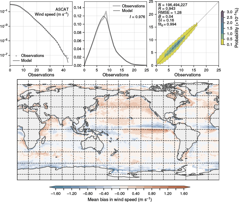
The bias correction defined in Eqn 1 is a simple threshold-based function. Other methods, such as quantile matching, can capture the probability of exceedance to a very high degree (Dowdy 2019). When applied to APS4 surface winds, the fit of the probability of exceedance and probability density is remarkable (top panels in Fig. 11). The figure legend and Table 4 show that the model skill improved for bias, slope, variability and probability density match. However, MAE, RMSE and SI are less favourable where errors increase. The bottom panel in Fig. 11 shows that quantile matching overestimates surface winds, particularly in the Northern Hemisphere. Results from the wave model confirm that the skill across the entire range of metrics is less than for the APS3 version, with RMSE above 0.40 m and a bias in order of 0.18 m (R = 0.966; SI = 0.14). The decrease in skill makes quantile matching for NWP wind correction less applicable to a dynamic wave model.
Satellite verification statistics for marine winds from ACCESS-G4 with quantile matching applied. The top panels show the probability of exceedance (left), probability density function and scatter density (right). The bottom panel shows spatial mean bias. Statistics were averaged globally from July 2023 to August 2024.
In the wave model, the drag coefficient converts the surface wind speed to surface stress in the wave-boundary layer; however, the shape of the function used to describe the drag coefficient is not entirely understood. The traditional algorithm for low to moderate winds is well established and fits observations for wind speeds of 2–20 m s−1 (Fairall et al. 2003). Above 20 m s−1, observations and modelling suggest that the drag should saturate and decrease to allow the development of severe storms like tropical cyclones (Edson et al. 2013; Soloviev et al. 2014). It would allow for higher values in the tail of wind speed distribution without overestimating the wave field.
Section 2 verified Hs from the global wave model and reanalysis with satellite altimeters. The AUSWAVE-G models compare very well against satellite observations to the point where they outperform the reanalysis. Reanalysis implies that some form of data assimilation is employed. In the case of ERA5, an optimal interpolation of altimeter data within the data assimilation window at hourly time intervals is performed (Hersbach et al. 2020). Therefore, altimeter data are not independent for ERA5, whereas for AUSWAVE, they are entirely independent. The fact that AUSWAVE, without data assimilation, outperforms ERA5 further strengthens our results.
In general, wave models can predict open ocean conditions very well. One would expect equivalent skill at the coast around Australia, but satellite and wave observations are not the same. Noticeable differences exist between the two. Wave buoys calculate the wave spectrum from time-series analysis at a single point on the sea surface for 20–40 min. Satellite altimeters integrate the illuminated area (instantaneous) over a spatial footprint on the sea surface and estimate significant wave height from the shape of the return signal. Besides instrumentation and sampling, wave buoys are affected by littoral and shallow water processes and the interaction of the ocean with the coast. It leads to greater scatter in verification with wave buoys than with altimeters, as shown in scatter density and time series plots in Section 3. The scatter is more evident in wave period (Fig. 9) than in significant wave height (Fig. 8).
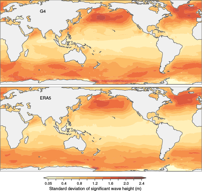
Finally, this study highlighted the need to consider the complete set of verification metrics. Although the ERA5 reanalysis performed best at bulk statistics, such as RMSE, SI and R, it could not capture the tail of the wind speed distribution and its variability (standard deviation). On the other hand, the NWP model can represent the tail and variability in surface winds but is less skilful regarding bulk statistics. For the wave field, the increased variability, relative to the ERA5 reanalysis, is localised to high latitudes and is primarily found in the North Pacific, North Atlantic and Southern Ocean (Fig. 12). In the tropics, the increase in variability is less pronounced but still evident across tropical cyclone paths in the north Indian Ocean and eastern Pacific. Besides tropical cyclone regions, the Mediterranean and Arabian Seas show increased variability. The pattern of wave variability in the Arabian Sea coincides with the seasonal cross-equatorial wind phenomenon known as the Somali Jet.
5.Conclusion
This paper examined the characteristics of marine surface winds of the global NWP model ACCESS APS4. We analysed 12 months to cover all seasonal wind and wave climate variations. Satellite verification showed that the mean bias in wind speed improved significantly in APS4, nullifying our previous bulk flux scaling approach in APS3. This led to a threshold-based bias correction to address an underestimation in the tail of the wind speed distribution. Fig. 1, 3 and 8 neatly demonstrate the assumption that Hs scales with U10 and that when increasing the tail of the distribution of surface winds, one can increase the tail of the distribution of waves. It suggests some merit in saturation and decay of the drag coefficient with increasing wind speed, such as the Hwang (2011) parameterisation.
Satellite altimeter and wave buoy verification across 84 locations yield an increase in skill in most metrics, which are consistent with each other. Importantly, we found that the forecast error improved compared to APS3 across all lead times. Comparisons to the wave reanalysis ERA5 indicate that the Bureau’s global wave forecast system with statistical wind correction outperforms the reanalysis across a few metrics, including R, RMSE, B, SI, slope and standard deviation (which increases the variability). It is not region-specific and performs globally, including at high latitudes.
The bias correction allows for separating wind errors from the wave model parameterisations and focusing on more nuanced wave model components in the balance equation, such as the drag parameterisation function. In an ideal scenario, the wave model parameters should not change when applying a different wind-forcing product.
Data availability
The work used Australia’s Integrated Marine Observing System (IMOS) marine service information from the Australian Ocean Data Network portal. The Australian National Wave Archive contains buoy data from the following organisations: Manly Hydraulics Laboratory (part of the New South Wales Department of Planning, Industry and Environment); Bureau of Meteorology; Western Australia Department of Transport; Queensland Government Department of Environment, Science and Innovation; University of Western Australia; Flinders University; South Australian Research and Development Institute (SARDI); Deakin University, The University of Melbourne; the Victorian Department of Environment, Land, Water and Planning; and Pilbara Port Authority. We acknowledge the use of observations from the US National Data Buoy Center (part of NOAA) and commercial customers within Australia. ASCAT data are produced by Remote Sensing Systems and sponsored by the National Aeronautics and Space Administration (NASA). Data are available at https://www.remss.com/. The Radar Altimeter Database System (RADS) is the source of along-track altimetry data for Sentinel-3a, Sentinel-3b, Cryosat-2 and Jason-3 platforms. Young and Ribal (2022) provided coefficients for altimeter calibration.
Declaration of funding
This research was financially supported by the Australian Bureau of Meteorology.
References
Alday M, Accensi M, Ardhuin F, Dodet G (2021) A global wave parameter database for geophysical applications. Part 3: improved forcing and spectral resolution. Ocean Modelling 166, 101848.
| Crossref | Google Scholar |
Ardhuin F, Rogers E, Babanin A V, Filipot J-F, Magne R, Roland A, Van der Westhuysen A, Queffeulou P, Lefevre J-M, Aouf L, Collard F (2010) Semiempirical dissipation source functions for ocean waves. Part I: definition, calibration, and validation. Journal of Physical Oceanography 40(9), 1917-1941.
| Crossref | Google Scholar |
Brassington GB, Pugh T, Spillman C, Schulz E, Beggs H, Schiller A, Oke PR (2007) BLUElink: development of operational oceanography and servicing in Australia. Journal of Research and Practice in Information Technology 39(2), 151-162.
| Google Scholar |
Breivik Ø, Carrasco A, Haakenstad H, Aarnes OJ, Behrens A, Bidlot JR, Björkqvist JV, Bohlinger P, Furevik BR, Staneva J, Reistad M (2022) The impact of a reduced high-wind charnock parameter on wave growth with application to the North Sea, the Norwegian Sea, and the Arctic Ocean. Journal of Geophysical Research: Oceans 127(3), e2021JC018196.
| Crossref | Google Scholar |
Cardone VJ, Jensen RE, Resio DT, Swail VR, Cox AT (1996) Evaluation of contemporary ocean wave models in rare extreme events: the “Halloween Storm” of October 1991 and the “Storm of the Century” of March 1993. Journal of Atmospheric and Oceanic Technology 13(1), 198-230.
| Crossref | Google Scholar |
Durrant TH, Greenslade DJM, Simmonds I (2013) The effect of statistical wind corrections on global wave forecasts. Ocean Modelling 70, 116-131.
| Crossref | Google Scholar |
Edson JB, Jampana V, Weller RA, Bigorre SP, Plueddemann AJ, Fairall CW, Miller SD, Mahrt L, Vickers D, Hersbach H (2013) On the exchange of momentum over the open ocean. Journal of Physical Oceanography 43(8), 1589-1610.
| Crossref | Google Scholar |
Fairall CW, Bradley EF, Hare JE, Grachev AA, Edson JB (2003) Bulk parameterization of air–sea fluxes: Updates and verification for the COARE algorithm. Journal of Climate 16(4), 571-591.
| Crossref | Google Scholar |
Gandoin R, Garza J (2024) Underestimation of strong wind speeds offshore in ERA5: evidence, discussion and correction. Wind Energy Science 9(8), 1727-1745.
| Crossref | Google Scholar |
GEBCO Bathymetric Compilation Group (2020) The GEBCO_2020 Grid – a continuous terrain model of the global oceans and land. (British Oceanographic Data Centre, National Oceanography Centre, NERC, UK) [Dataset] 10.5285/a29c5465-b138-234d-e053-6c86abc040b9
Hasselmann K (1960) Grundgleichungen der Seegangsvoraussage. Schiffstechnik 7(39), 191-195 [In German].
| Google Scholar |
Hasselmann S, Hasselmann K, Allender JH, Barnett TP (1985) Computations and parameterizations of the nonlinear energy transfer in a gravity-wave spectrum. Part II: parameterizations of the nonlinear energy transfer for application in wave models. Journal of Physical Oceanography 15(11), 1378-1391.
| Crossref | Google Scholar |
Hersbach H, Bell B, Berrisford P, Hirahara S, Horányi A, Muñoz-Sabater J, Nicolas J, Peubey C, Radu R, Schepers D, Simmons A, Soci C, Abdalla S, Abellan X, Balsamo G, Bechtold P, Biavati G, Bidlot J, Bonavita M, De Chiara G, Dahlgren P, Dee D, Diamantakis M, Dragani R, Flemming J, Forbes R, Fuentes M, Geer A, Haimberger L, Healy S, Hogan RJ, Hólm E, Janisková M, Keeley S, Laloyaux P, Lopez P, Lupu C, Radnoti G, de Rosnay P, Rozum I, Vamborg F, Villaume S, Thépaut JN (2020) The ERA5 global reanalysis. Quarterly Journal of the Royal Meteorological Society 146(730), 1999-2049.
| Crossref | Google Scholar |
Hwang PA (2011) A note on the ocean surface roughness spectrum. Journal of Atmospheric and Oceanic Technology 28(3), 436-443.
| Crossref | Google Scholar |
Janssen PAEM (1991) Quasi-linear theory of wind-wave generation applied to wave forecasting. Journal of Physical Oceanography 21(11), 1631-1642.
| Crossref | Google Scholar |
Janssen P (1998) On error growth in wave models. ECMWF Technical Memoranda 249, 12.
| Crossref | Google Scholar |
Janssen PAEM, Bidlot JR (2018) Progress in operational wave forecasting. Procedia IUTAM 26, 14-29.
| Crossref | Google Scholar |
Liu Q, Rogers WE, Babanin A V, Young IR, Romero L, Zieger S, Qiao F, Guan C (2019) Observation-based source terms in the third-generation wave model WAVEWATCH III: updates and verification. Journal of Physical Oceanography 49(2), 489-517.
| Crossref | Google Scholar |
Liu Q, Babanin A V, Rogers WE, Zieger S, Young IR, Bidlot JR, Durrant T, Ewans K, Guan C, Kirezci C, Lemos G, MacHutchon K, Moon IJ, Rapizo H, Ribal A, Semedo A, Wang J (2021) Global wave hindcasts using the observation-based source terms: description and validation. Journal of Advances in Modeling Earth Systems 13(8), e2021MS002493.
| Crossref | Google Scholar |
Meucci A, Young IR, Pepler A, Rudeva I, Ribal A, Bidlot JR, Babanin A V (2023) Evaluation of spectral wave models physics as applied to a 100-year Southern Hemisphere extra-tropical cyclone sea state. Journal of Geophysical Research: Oceans 128(9), e2023JC019751.
| Crossref | Google Scholar |
National Operations Centre (2020) APS3 upgrade of the ACCESS-G/GE Numerical Weather Prediction system, Bureau Operational Bulleting number 125. (Bureau of Meteorology: Melbourne, Vic., Australia) Available at http://www.bom.gov.au/australia/charts/bulletins/opsbull_G3GE3_external_v3.pdf
Oladejo HO, Bernstein DN, Cambazoglu MK, Nechaev D, Abdolali A, Wiggert JD (2025) Wind forcing, source term and grid optimization for hurricane wave modelling in the Gulf of Mexico. Coastal Engineering 197, 104692.
| Crossref | Google Scholar |
Pathirana S, Young I, Meucci A (2023) Modelling swell propagation across the Pacific. Frontiers in Marine Science 10, 1187473.
| Crossref | Google Scholar |
Rogers WE, Wittmann PA, Wang DWC, Clancy RM, Hsu YL (2005) Evaluation of global wave prediction at the fleet numerical meteorology and oceanography center. Weather and Forecasting 20, 745-760.
| Crossref | Google Scholar |
Saha S, Moorthi S, Wu X, Wang J, Nadiga S, Tripp P, Behringer D, Hou Y-T, Chuang H-Y, Iredell M, Ek M, Meng J, Yang R, Mendez MP, van den Dool H, Zhang Q, Wang W, Chen M, Becker E (2014) The NCEP climate forecast system version 2. Journal of Climate 27(6), 2185-2208.
| Crossref | Google Scholar |
Schulz EW, Josey SA, Verein R (2012) First air–sea flux mooring measurements in the Southern Ocean. Geophysical Research Letters 39(16), L16606.
| Crossref | Google Scholar |
Soloviev A V, Lukas R, Donelan MA, Haus BK, Ginis I (2014) The air–sea interface and surface stress under tropical cyclones. Scientific Reports 4, 5306.
| Crossref | Google Scholar | PubMed |
Stopa JE, Ardhuin F, Babanin A, Zieger S (2016) Comparison and validation of physical parameterizations in spectral wave models. Ocean Modelling 103, 2-17.
| Crossref | Google Scholar |
Swain MJ, Ballard DH (2002) Color indexing. In ‘Readings in Multimedia Computing and Networking’. (Eds K Jeffay, N Zhang) pp. 265–277. (Elsevier) 10.1016/B978-155860651-7/50109-1
Thomson J, D’Asaro EA, Cronin MF, Rogers WE, Harcourt RR, Shcherbina A (2013) Waves and the equilibrium range at Ocean Weather Station P. Journal of Geophysical Research: Oceans 118(11), 5951-5962.
| Crossref | Google Scholar |
Tolman HL (1998) Validation of NCEPs ocean winds for the use in wind wave models. Global Atmosphere and Ocean System 6, 243-268.
| Google Scholar |
Tolman HL, Balasubramaniyan B, Burroughs LD, Chalikov D V, Chao YY, Chen HS, Gerald VM (2002) Development and implementation of wind-generated ocean surface wave models at NCEP. Weather and Forecasting 17(2), 311-333.
| Crossref | Google Scholar |
Tolman HL, Banner ML, Kaihatu JM (2013) The NOPP operational wave model improvement project. Ocean Modelling 70, 2-10.
| Crossref | Google Scholar |
Valiente NG, Saulter A, Edwards JM, Lewis HW, Sanchez JMC, Bruciaferri D, Bunney C, Siddorn J (2021) The impact of wave model source terms and coupling strategies to rapidly developing waves across the north‐west European shelf during extreme events. Journal of Marine Science and Engineering 9(4), 403.
| Crossref | Google Scholar |
Valiente NG, Saulter A, Gomez B, Bunney C, Li JG, Palmer T, Pequignet C (2023) The Met Office operational wave forecasting system: the evolution of the regional and global models. Geoscientific Model Development 16(9), 2515-2538.
| Crossref | Google Scholar |
Wiese A, Staneva J, Ho-Hagemann HTM, Grayek S, Koch W, Schrum C (2020) Internal model variability of ensemble simulations with a regional coupled wave–atmosphere model GCOAST. Frontiers in Marine Science 7, 596843.
| Crossref | Google Scholar |
Young IR, Babanin AV, Zieger S (2013) The decay rate of ocean swell observed by altimeter. Journal of Physical Oceanography 43(11), 2322-2333.
| Crossref | Google Scholar |
Young IR, Ribal A (2022) Can multi-mission altimeter datasets accurately measure long-term trends in wave height? Remote Sensing 14(4), 974.
| Crossref | Google Scholar |
Zieger S, Greenslade D (2021) A multiple-resolution global wave model – AUSWAVE-G3, Bureau Research Report Number 51. (Bureau of Meteorology: Melbourne, Vic., Australia) Available at http://www.bom.gov.au/research/publications/researchreports/BRR-051.pdf
Zieger S, Babanin AV, Rogers WE, Young IR (2015) Observation-based source terms in the third-generation wave model WAVEWATCH. Ocean Modelling 96, 2-25.
| Crossref | Google Scholar |

