

Projected climate change in Australian marine and freshwater environments
Alistair J. Hobday A C and Janice M. Lough BA Climate Adaptation Flagship, CSIRO Marine and Atmospheric Research, Hobart, Tas. 7001, Australia.
B Australian Institute of Marine Science, PMB 3, Townsville MC, Qld 4810, Australia.
C Corresponding author. Email: alistair.hobday@csiro.au
Marine and Freshwater Research 62(9) 1000-1014 https://doi.org/10.1071/MF10302
Submitted: 1 December 2010 Accepted: 29 July 2011 Published: 21 September 2011
Journal Compilation © CSIRO Publishing 2011 Open Access CC BY-NC-ND
Abstract
Changes in the physical environment of aquatic systems consistent with climate change have been reported across Australia, with impacts on many marine and freshwater species. The future state of aquatic environments can be estimated by extrapolation of historical trends. However, because the climate is a complex non-linear system, a more process-based approach is probably required, in particular the use of dynamical projections using climate models. Because global climate models operate on spatial scales that typically are too coarse for aquatic biologists, statistical or dynamical downscaling of model output is proposed. Challenges in using climate projections exist; however, projections for some marine and freshwater systems are possible. Higher oceanic temperatures are projected around Australia, particularly for south-eastern Australia. The East Australia Current is projected to transport greater volumes of water southward, whereas the Leeuwin Current on the western coast may weaken. On land, projections suggest that air temperatures will rise and rainfall will decline across much of Australia in coming decades. Together, these changes will result in reduced runoff and hence reduced stream flow and lake storage. Present climate models are particularly limited with regard to coastal and freshwater systems, making the models challenging to use for biological-impact and adaptation studies.
Additional keywords: climate-change impacts, freshwater fishes, future climate scenarios, global climate model, marine fishes.
Introduction
The climate of Australia’s marine environments has already changed compared with historical baselines (Lough 2008; Poloczanska et al. 2009; Lough and Hobday 2011). On both eastern and western coasts, water temperatures have warmed and salinity has increased in the poleward-flowing currents (Pearce and Feng 2007; Ridgway 2007). In the ocean surrounding Australia, these physical changes coincide with biological changes in a range of marine species, including changes in local abundance, geographic range, phenology and community structure (e.g. Hobday et al. 2007; Poloczanska et al. 2007; Figueira and Booth 2010; Last et al. 2011). Climate change is already affecting many marine fishes and other organisms, although its effects are often exacerbated or concealed by chronic and widespread anthropogenic disturbances.
Given the physical changes observed over the Australian continent, for example in air temperature and rainfall (e.g. Hughes 2003; CSIRO 2007; Hennessy et al. 2007), it is likely that freshwater environments such as rivers and lakes are also being affected, although the evidence is less coherent (Lough and Hobday 2011). Changes in vegetation cover have exacerbated the effects of higher temperatures caused by climate change, resulting in longer-lasting and more severe droughts (e.g. Deo et al. 2009; Ummenhofer et al. 2009). The droughts and general drying in some parts of the country have reduced runoff into fish habitats such as estuaries, rivers and lakes. Victoria has seen a decline in autumn rainfall of 40% in the period 1950–2006 (Cai and Cowan 2008a). In the Murray–Darling Basin, rainfall has declined by 11% since 1950, yet river flow has declined 55% below the long-term average (Steffen 2009). An increase of 1°C in air temperature has been associated with a 15% reduction in stream flow over this period (Cai and Cowan 2008b). In south-western Western Australia, stream flow into dams and reservoirs has fallen dramatically since the early 1900s, from an average of 338 GL before 1974, to less than 90 GL for the period 2001–2006 (Steffen 2009). Since 2006, stream flow has declined even further (http://www.watercorporation.com.au/D/dams_storage.cfm, accessed 24 August 2011).
Given the sustained and ongoing emissions of greenhouse gases, and the long residence time of carbon dioxide (CO2) in the atmosphere, future changes are inevitable (IPCC 2007; Solomon et al. 2009). At a global scale, climate change that takes place as a result of increases in CO2 concentration is considered to be largely irreversible for 1000 years after emissions stop (Solomon et al. 2009). Sea level, temperature and ocean pH will continue to change over the coming centuries (IPCC 2007), with major effects on biological systems. However, immediate reductions in greenhouse-gas emissions are still important to limit future impacts below dangerous levels (e.g. Schneider 2009).
Planning for adaptation responses requires information on the expected condition of future ocean and freshwater environments. Timely development of appropriate adaptation strategies should increase the flexibility in management of vulnerable species and ecosystems (Hulme 2005). Thus, access to information on future climate is critical for many biologists and managers working to determine species and ecosystem impacts. In the present paper, we first explain how climate projections are obtained, discussing some of the associated caveats and limitations. We then provide a range of projections for Australia’s aquatic environments. Given the rapid progress in development of climate projections, improving the ability of aquatic scientists, managers and policy makers to access the most up-to-date and appropriate projections will lead to a range of benefits in delivering better biological projections, and is a major goal of the present paper. In turn, improved biological projections will underpin appropriate adaptation strategies and decision-making.
Projecting future conditions
One way to estimate future environmental conditions is simply to extrapolate on the basis of historical trends. This approach is not widely used because it would be useful only over short time periods (decades at best) and may not allow for dynamical (non-linear) changes in the ocean–atmosphere system. In principle, it could be used to examine near-term changes; however, on these time scales, natural climate variability tends to obscure climate trends. Future conditions for the Earth’s climate system will depend not only on the planet’s system response to changes in greenhouse-gas concentrations and radiative forcing, but also on how humans respond through changes in technology, economies, lifestyle and policy (Moss et al. 2010). To account for that wide range of possible futures, the Intergovernmental Panel on Climate Change (IPCC) developed alternative future emission scenarios to be used for driving global models (see fig. 1 in Moss et al. 2010). A set of scenarios known as Special Report on Emissions Scenarios (SRES) was used in the Third Assessment Report (TAR) in 2001 and the Fourth Assessment Report (AR4) in 2007 (IPCC 2007) (Fig. 1). These scenarios represent a range of warming, and have been widely used in biological studies (e.g. Anthony et al. 2008; Hobday 2010). Relatively low (e.g. SRES B1, CO2 concentration stabilisation at 549 ppm by 2100 and global temperatures ∼2–4°C higher than the 1990 levels), medium (e.g. A1B, 717 ppm of atmospheric CO2 by 2100 and global temperatures ∼3–5°C higher) and high (e.g. A1FI, 970 ppm of atmospheric CO2 by 2100 and global temperatures ∼5–6°C higher) scenarios are often used in projection studies as a way of bracketing the future change. However, given the present rates of greenhouse-gas emissions and observed climate change (Rahmstorf et al. 2007; Le Quéré et al. 2009), low scenarios are now seen as less realistic. For the period up to 2030, all the scenarios are similar, and then diverge to the end of the century.

|
Unfortunately, just as biologists and other ‘user’ scientists were becoming familiar with these scenarios and their nomenclature, an updated set of scenarios is now being used for IPCC AR5, based on radiative forcing (Moss et al. 2010). Radiative forcing describes a change in the radiation balance, such as may be caused by changes in atmospheric concentrations of greenhouse gases. Positive forcing, for example, drives warming of the Earth system. These new four main scenarios, known as Representative Concentration Pathways (RCP), differ from the SRES set in that they include scenarios that allow for climate-change mitigation and adaptation (Fig. 1). The four main RCPs, namely RCP 8.5, RCP 6.0, RCP 4.5 and RCP 2.6, correspond to CO2 equivalent (CO2 plus other greenhouse gases) concentrations of 1370, 850, 650 and 490 ppm in 2100 (Moss et al. 2010). Although the currency has changed (gas concentration (ppm) to radiative forcing (W m–2)), the SRES and RCPs are related in that increasing concentrations of greenhouse gases affect the balance between incoming solar radiation and outgoing heat radiation which determines the Earth’s average temperature. Previously, SRES greenhouse-gas concentrations were converted to radiative forcing of the climate system by using radiation conversion codes located within each global climate model (GCM), which represented an unnecessary additional source of variation now removed under the RCP approach (Moss et al. 2010). Biologists will likely continue to use the SRES scenarios for some time, because many climate models and projections are based on these scenarios. A similar lag and transition period occurred when the IS92 scenarios used in the Second Assessment Report of 1995 were superseded by the SRES set (e.g. Orr et al. 2005; Poloczanska et al. 2007).
Alternative emission scenarios presented by the IPCC are global and based on changes in greenhouse-gas concentrations (SRES) or radiative forcing (RCP), necessitating complex conversion into a range of relevant climate variables at finer scales, using GCMs developed by several research organisations around the world. These models are based on the general principles of fluid dynamics and thermodynamics and have their origin in weather prediction (Stute et al. 2001). GCMs describe the dynamics of the atmosphere and ocean in an explicit way, typically at horizontal spatial scales of 1–3 degrees, and with varying numbers of vertical layers in the ocean and atmosphere, and provide a way to run quantitative experiments on climate conditions during the past, present and future. Advances in development of GCMs used for climate modelling are typically oriented around the IPCC reporting timelines, with transition periods as for emission scenarios when both old and new models are available to the wider research community.
Uncertainties in future projections based on climate models should not be underestimated, and result from a combination of scenario uncertainty (what will be the future level of greenhouse-gas emissions), climate sensitivity to these emissions, difference among climate models (e.g. how each model incorporates ocean–land–atmosphere processes) and model scale (IPCC 2007). Although single model–scenario combinations may have considerable uncertainty, there are several approaches to improve confidence in future projections such that dependent biological projections can be useful, as outlined in the following sections. However, all model outputs consistently show that rates of warming are likely to increase to the end of this century, unless there is an immediate and marked reduction in greenhouse-gas emissions (Schneider 2009).
Future IPCC projections have been used to justify and design biological and ecological studies on effects of climate change (e.g. Anthony et al. 2008; Byrne et al. 2009). The challenge for biologists is to identify a restricted number of appropriate experimental treatments that are not only relevant to the specific regional setting for their studies (contingent on appropriate downscaling), but that also account for different temporal scales of interest. For example, there are several instances where clear thresholds have been identified from experimental studies (Anthony et al. 2008; Byrne et al. 2009) and the challenge then is to assess when or how often this threshold is likely to be exceeded in future. Care should be taken in using future projections because considerable uncertainty is known to exist for some variables, areas and models. Partnership with climate modellers is recommended when using projections for the first time. We encourage such cross-disciplinary collaboration that will lead to more integrated biological projections; the present paper should help inform conversations between biologists and climate modellers.
Which model to use and how to get it
Biologists can be challenged in several ways in their attempts to use data from the range of available GCMs. Model selection and validation, model scale and model access can all be problematic. The first two issues will be discussed briefly before we describe how to access model data and use examples to illustrate potential future environmental conditions in Australian aquatic environments.
Not all climate models perform equally well for all variables in all regions. Whereas the ability of models to project future conditions cannot be assessed, performance in reproducing current climate conditions and historical patterns can be assessed. For example, Suppiah et al. (2007) used statistical methods to test how well 23 AR4 models simulated observed average patterns of mean sea-level pressure, temperature and rainfall over the Australian region. They then used the 15 best models to derive projections for 2030 and 2070 for the variables of interest. This process, known as validation, is considered best practice when attempting to use GCMs to forecast future conditions. Unfortunately, the observational data to validate models are often not available for aquatic biologists, nor are they within their typical skill set. Thus, using a suite of models to make an ensemble average will be the best available option for marine and freshwater researchers, although there is some debate as to whether this approach provides the most robust projections for regionally specific climate-change projections, because inclusion of poor models can bias the ensemble average (Perkins et al. 2009; Pierce et al. 2009; Shukla et al. 2009; Smith and Chandler 2010). Even though the resolution of climate models is improving, model scale is still considered coarse (∼100–200 km) with regard to representation of the environmental and biological processes that many aquatic biologists are interested in (<10 km), such as reef-specific recruitment or growth. Thus, downscaling of climate models is considered necessary before projections are meaningful.
In this context, downscaling is the process of transforming information from coarse-resolution GCMs to a finer regional spatial resolution. Downscaling is necessary where the mesoscale processes (in the ocean, these operate at scales of <100 km) are very sensitive to local climate, and the drivers of local climate variations, such as topography, are not captured at coarse scales. There are two broad categories of downscaling, namely dynamic (which simulates physical processes at fine scales) and statistical (which transforms coarse-scale climate projections to a finer scale, on the basis of observed relationships between the climate at the two spatial resolutions) (e.g. Whetton et al. 2005; Schmidli et al. 2006; Vasiliades et al. 2009; Tabor and Williams 2010).
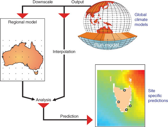
Dynamic downscaling uses regional climate models (RCMs) to translate the large-scale weather and ocean evolution from a GCM into a physically consistent evolution at higher resolution (Tabor and Williams 2010) (Fig. 2). Marine RCMs represent the processes that are subgrid scale in the GCMs, which makes them computationally expensive, because they solve multiple equations regarding the transfer of heat and energy in multiple depth layers at time steps as short as 30 min. Statistical downscaling is based on empirical relationships between the regional climate (e.g. local sea-surface temperature, SST) and large-scale predictor variables (e.g. heat content in the tropical ocean) derived from the GCM. Advantages include computational simplicity and that large-scale predictors can be relatively robust in terms of the relationship with local variables. Different relationships occur in different regions, thus downscaling must be calculated anew for each study region. This approach assumes that the relationship between large-scale processes and local variables is stationary over time (Tabor and Williams 2010). This assumption is unlikely to be met over longer time scales, and is a fundamental problem with statistical downscaling. The relationship between variables is projected to change in future, such that present combinations of climate variables cease to occur and are replaced by novel combinations (Williams et al. 2007).
|
The primary source of information on future projections comes from the output of GCMs, such as, for example, the set of World Climate Research Program CMIP3 models used to support the IPCC AR4. The volume of data from these GCMs can be overwhelming and disparate in file structure and notation. Central repositories were established to facilitate access to consistently formatted model output (www2-pcmdi.llnl.gov/esg_data_portal, accessed 24 August 2011). However, downloading and accessing complete suites of data requires independent data programming. Recently, data portals have been developed that allow extraction of the desired data without downloading the original files (e.g. http://www.ipcc-data.org/ddc_visualisation.html, accessed 24 August 2011). These data are coarse in time (e.g. monthly fields) and space and, in the case of marine waters, do not resolve mesoscale features such as eddies, coastal upwelling, realistic boundary currents or fronts (Fig. 3a). At this resolution, only broad latitudinal patterns of warming can be seen.

|
Secondary processing of GCM data (e.g. Whetton et al. 2005; Harwood et al. 2010; Tabor and Williams 2010) offers some options for biologists; however, the flexibility of data selection and limited number of variables available can be problematic. A set of GCM ensembles for the Australian region was released in 2007, and allows web-based access to a limited set of variables for a range of time periods and seasons (www.climatechangeinaustralia.gov.au, accessed 24 August 2011). For marine users, only a single variable is available (SST), although wind-speed projections also cover the ocean region. For freshwater users, only proxies such as air temperature, solar radiation, potential evapotranspiration and rainfall are available. The spatial resolution in these products is again quite coarse (0.1°), and mesoscale features are not resolved (Fig. 4). At this stage, the raw data cannot be downloaded from this portal.
|
Finer-scale data are currently available via rescaled GCMs (statistical downscaling based on pattern matching in OzClim and OzClim for Oceans, www.csiro.au/ozclim/home.do, accessed 24 August 2011; Whetton et al. 2005), again with a limited number of variables for aquatic users (marine: SST, temperature at a depth of 250 m, and salinity; freshwater: rainfall, potential evapotranspiration, air temperature). Even though the resolution is improved, mesoscale features are still not resolved, although in the ocean, the major boundary currents on the eastern and western coasts of Australia can be detected (Fig. 3b). This data source may be the most useful for biologists seeking general patterns of future change, and has been widely used to inform managers and policy makers in a range of terrestrial sectors. More recently, even finer-scale downscaling for terrestrial variables has been completed by using the OzClim data, with a topographical correction at a scale of 1 km2 (Harwood et al. 2010).
At present, dynamical downscaling approaches using RCMs for the Australian region are ‘experimental’ only. For example, in the ocean, the Bluelink model (Oke et al. 2008) has been nested in the CSIRO Mk3.5 model and has a limited number of future years (2063–2065) of data at a 10-km resolution, that are useful in projecting future habitat distribution of marine species (e.g. Hartog et al. 2011). Mesoscale features are resolved (e.g. Fig. 3c), although there are ongoing challenges with evaluating the reliability of the downscaling (M. A. Chamberlain, C. Sun, R. J. Matear and M. Feng, unpubl. data). Tabor and Williams (2010) discussed some additional limitations with downscaling GCMs to a finer resolution.
We now illustrate some of the future projections for Australian aquatic environments out to the Year 2100 on the basis of a variety of these approaches. We encourage biologists to become primary users of climate-model output through one of the access options described above. Both absolute values and relative changes compared with a baseline period are used by biologists for both experimental studies and predictive biological models, and we use both styles of projection in the following sections.
Australia’s future aquatic climate
At a national scale, a recent summary by the CSIRO and the Bureau of Meteorology (BOM) indicated that Australian average air temperatures are projected to rise by 0.6–1.5°C by 2030, relative to 1990 temperatures (State of the Climate 2010). If global greenhouse-gas emissions continue to grow at present rates, warming is projected to be in the range of 2.2–5.0°C by 2070. Warming is projected to be lower near the coast and in Tasmania because the oceans (and adjacent land masses) warm at a slower rate than do more inland areas, and areas higher in central and north-western Australia. These changes will be felt through an increase in the number of hot days. Thus, drying and decreased runoff into freshwater habitats is also likely. While direct projections of stream flow are not available, historical relationships between declines in rainfall and stream flow suggest that a 1 : 4 reduction ratio is realistic (e.g. Steffen 2009).
Warming is also expected in seas around Australia. By the 2030s, SSTs are projected to be ∼1°C higher (than those in 1980–1999) around Australia, with slightly less warming in southern Australia. By the 2070s, SSTs are projected to be 1.5–3.0°C higher (on the basis of SRES scenarios), with slightly less warming to the south of the continent and the greatest warming east and north-east of Tasmania (Poloczanska et al. 2007; Lough 2009).
Marine environments
The marine environments of Australia range from coastal bays and estuaries, near-shore shallows and reefs, across the continental shelf to the deep ocean where depths exceed 3000 m (e.g. Poloczanska et al. 2007). Monitoring in this environment is very limited, and many gaps in time series and spatial coverage exist (e.g. Lough and Hobday 2011). The advent of satellite-based measurements has allowed synoptic coverage, but only of near-surface properties such as SST, ocean colour and sea-surface height. Thus, projections of change in variables derived via GCMs for historical periods (hindcasts) cannot always be validated against historical observations. In the following sections, we provide examples of projected future change in variables that are relevant to marine species, including SST, sea level, ocean currents, ocean chemistry and extreme events.
Sea-surface temperature
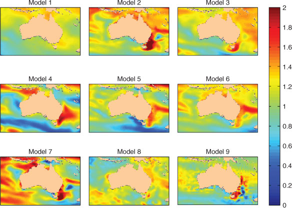
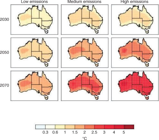
Projections of SST based on a suite of climate models used for IPCC AR3 and AR4 downscaled with the OzClim approach (Whetton et al. 2005) show considerable variability in some parts of Australia, such as north-western Australia (Fig. 5). In south-eastern Australia, there is more agreement among model projections, and warming appears in all model realisations. When an ensemble average is generated, south-eastern Australia shows the greatest projected rate of warming to the end of this century, as a result of both atmospheric warming and the EAC intensification. By 2050, average temperatures in this region are projected to be 2°C higher than the 1990–2000 average (Fig. 6). In contrast, much less warming is evident in the upwelling regions of western Victoria, which has been attributed to increased upwelling (Hobday et al. 2007). Biologists seeking to determine appropriate temperature rises to use in experimental work should select a range of temperatures around a mean value in their region of interest to account for inter-model variability, and to ensure that results remain relevant, even as scenarios change.
|

|
Sea level
Globally, sea levels are currently rising at the upper end of current projections (Rahmstorf et al. 2007). Sea level will continue to rise during the 21st century and beyond in response to increasing concentration of greenhouse gases. The IPCC projections are for a global sea-level rise of 18–79 cm by 2095, compared with 1990 (IPCC 2007; Church et al. 2009). However, there is limited understanding of the response of ice sheets to global warming and a larger rise is possible. Rising sea levels will result in inundation of low-lying coastal regions and greater coastal erosion, which will be particularly critical for estuarine habitats (Gillanders et al. 2011). Coastal sea-level rise and resulting impacts are elevated during storm events and at times of high tides. Where coastlines are highly modified, such as in the densely populated south-east of Australia, the ability of coastal species and habitats such as mangroves to naturally adapt to sea-level rise and migrate landwards is reduced; a process referred to as the ‘coastal squeeze’ (Church et al. 2009). As for temperature, sea-level rise will not be uniform around Australia; however, confidence in regional projections is low because GCMs show little agreement at this scale (Church et al. 2009). That caveat noted, the average from 17 climate-model simulations based on the A1B scenario suggest a higher than global average sea-level rise off the south-eastern coast of Australia for both 2030 and 2070 (see Church et al. 2009).
Ocean currents
The observed warming along the eastern coast of Australia is associated with systematic changes in the surface currents, including strengthening of the East Australia Current (EAC) and increased southward flow as far south as Tasmania (Cai et al. 2005; Poloczanska et al. 2007; Ridgway 2007). Historical change in the EAC has been explained by a southward migration of the high-latitude westerly wind belt south of Australia (Cai 2006). In turn, this movement of the wind belt has been attributed to both ozone depletion and increases in greenhouse gases (Gillett and Thompson 2003). Climate-model simulations show consensus that these trends will continue over the next 100 years, with Cai et al. (2005) reporting a 20% increase in the mean flow of the EAC by 2070, on the basis of projections using CSIRO Mk3. This continued intensification will compound the direct regional warming caused by increased solar radiation received at the surface. This eastern-coast region is projected to remain a globally important hotspot of climate change for at least the next 50 years (A. J. Hobday and G. Pecl, unpubl. data).
Along the western coast of Australia, the Leeuwin Current (LC) also carries warm water southward, but the smaller transport volume of this current makes projection more difficult than for the EAC (Hobday et al. 2007; Poloczanska et al. 2007). From the mid-1970s to mid-1990s, a trend of subsurface cooling in the equatorial western Pacific, coupled with a weakening trend of the Pacific trade winds, was transmitted into the south-eastern Indian Ocean and the LC region and caused a multi-decadal weakening of the LC strength. Since the mid-1970s, the volume transported in the LC has declined by 10–30%, and thus its southward heat transport has also declined (Feng et al. 2009). Despite this decline in transport, there have been persistent warming trends and an increase in salinity in the LC and associated shelf waters over the past 50 years (Pearce and Feng 2007).
Although change in the LC is difficult to directly project from climate models because of scale issues, more recent analysis of climate-model simulations suggest that the LC trend is related to reductions of trade-wind strength in the tropical Pacific, increase in the frequency of Indian Ocean Dipole events, and the upward trend of the Southern Annular Mode (SAM). The LC trend in recent decades is mostly due to the effect of increased greenhouse gases in the atmosphere, although ozone depletion has also played a role in the trend of the SAM (Cai et al. 2005). Climate-model projections suggest that these climate trends are likely to continue in the future. Therefore, on the basis of these various indicators, the LC could continue to weaken slowly in future years (Feng et al. 2009).
In the south, the Great Australian Bight region will experience more westward transport from the Indian Ocean as global temperatures rise, but a reduction in the strength of the LC will mean reduced coastal flow to the east. Along the north-western and north-eastern coasts, an increase in the northward flow water has been projected (Poloczanska et al. 2007).
Ocean chemistry
The pH of the surface oceans is projected to decrease by 0.2–0.3 units by 2100 (Orr et al. 2005; Howard et al. 2009). As for sea level, regional projections around Australia are difficult to make, and global averages are the most robust estimates currently available because surface ocean chemistry largely tracks atmospheric concentrations of CO2. That said, spatial variation in projected change around Australia does exist, and a single model projection is used as an example (Fig. 7). Oceanic pH is lower in north-eastern Australia, and continues to decline to lower levels by 2100. The aragonite saturation state is initially higher in northern Australian waters, but is projected to drop below 3 by 2060. Calcite saturation state also declines to the end of the century (Fig. 7).

|
Of critical importance for marine calcifying organisms is when pH drops to levels where waters become under-saturated in carbonate (in the form of the more soluble aragonite or less soluble calcite). This is because, without additional energy being expended to maintain structural carbonate, weaker structures result (e.g. Doney et al. 2009) and even dissolution is possible (e.g. Howard et al. 2009). Around Australia, the time at which saturation states approach these thresholds varies (Fig. 7).
The acidity of ocean waters, and the saturation states, can vary on daily, seasonal and inter-annual time scales, and much work remains to be conducted to understand the effect of variation in pH for biology. In the high-latitude Southern Ocean, aragonite saturation thresholds may be crossed in winter by about 2040 (McNeil and Matear 2008). By 2100, the surface of the entire Southern Ocean (south of the Polar Front) is projected to become under-saturated for aragonite (Orr et al. 2005). Declining aragonite saturation states in tropical waters have already been implicated in declining coral growth rates (De’ath et al. 2009), and this trend is expected to continue, threatening the structure of coral-reef communities as they exist today (Hoegh-Guldberg et al. 2007). Tropical fish may also be affected, in ways that are only becoming apparent as a result of novel experiments (e.g. Munday et al. 2009; Pankhurst and Munday 2011). Aragonite saturation horizons will occur at shallower depths in future, especially in the Antarctic and Australian southern margins, threatening a wide range of larval and adult benthic and pelagic calcifying organisms (e.g. Przeslawski et al. 2008; Sheppard Brennand et al. 2010).
Freshwater environments
Climate projections for freshwater environments are not available at a national scale. Water bodies such as rivers and lakes are below the resolution of grid cell-based GCMs, and trend or statistical analysis is required to generate local projections on the basis of proxy data such as air temperature, solar radiation, evaporation rates and rainfall. General patterns are illustrated for air temperature and rainfall, with additional data projections freely and easily available, as described in previous sections.
Surface-air temperatures
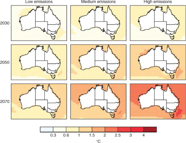
Air temperatures in the Australian region are projected to continue to rise through the 21st century, with a magnitude comparable to the global average. Atmospheric temperatures over land are projected to rise more than those of the surrounding ocean, with slightly less warming in Tasmania and coastal regions (see Lough 2009). Ensemble projections based on multi-modal averages show that warming relative to the 1980–1999 baseline is greatest in north-western Australia, with an increase of 2.5°C by 2050 on the basis of a medium-emission scenario (A1B) for the average set of models (Fig. 8). Given current trends in global warming (Rahmstorf et al. 2007; Le Quéré et al. 2009), warming patterns observed from higher-emission scenarios (A1FI) are also likely. Warming patterns similar to those based on analyses presented in Suppiah et al. (2007) are obtained using the OzClim online scenario-generation tool for individual models and range of scenarios (www.csiro.au/ozclim, 24 August 2011). The spatial resolution in both projection sets is coarse (0.25 degrees), and for some biological uses, will not be suitable for resolving differences at local scales. When considering local scales, higher air temperatures may heat the water bodies, increasing stratification and lowering oxygen concentration, with negative effects on fish physiology (Ficke et al. 2007).
|
Rainfall and river-flow variability
Rainfall is generally projected to decline over most of Australia, with a small increase in the far north according to some models (Poloczanska et al. 2007). Confidence in these projections is, however, less than for temperature changes because there is relatively poor agreement as to the sign of the precipitation response over many parts of Australia. Even without significant changes in rainfall amounts, the effectiveness of rainfall will decrease because of warmer temperatures, as has already been observed in the climate record (Lough and Hobday 2011). At a regional scale, by 2070 for a medium emission scenario (SRES A1B), annual rainfall is projected to decline by 5–10% for south-eastern Australia and by 10–20% for south-western Australia (Fig. 9) (Suppiah et al. 2007). High-emission scenarios show these reductions occurring earlier, i.e. between 2030 and 2050. Seasonal differences are also apparent, with winter rainfall declining over most of the country, whereas summer rainfall may increase in some parts of northern Australia (Suppiah et al. 2007; see www.climatechangeinaustralia.gov.au, 24 August 2011). Salinity problems, which can occur throughout lower parts of a river system and are problematic in south-western Australia and the Murray–Darling regions, may be exacerbated by changes in rainfall, temperature and stream flows (Morrongiello et al. 2011; Pratchett et al. 2011). Lower flows and higher temperatures may also reduce water quality within the catchment. For example, low flows, higher temperatures and elevated nutrients create a more favourable environment for potentially harmful algal blooms.
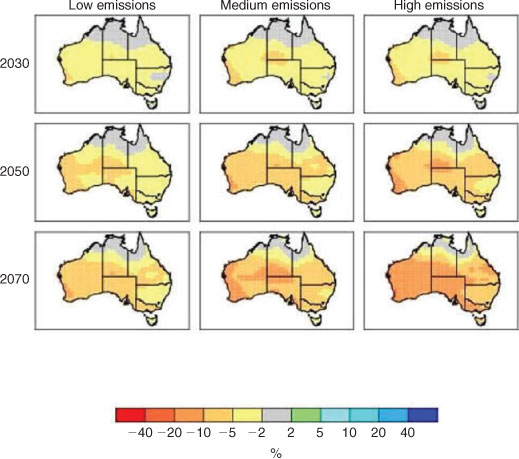
|
Projections of rainfall and temperature at finer scales, down to 1 km2, are being generated for several regions on the basis of the OzClim data, and involve combining a pattern of observed historical rainfall distribution with the coarser OzClim projections. This ‘correction’ can be used to generate finer patterns. Corrections for topography have also been used (e.g. Harwood et al. 2010; Fig. 10) and the software to generate these downscaled scenarios is publicly available (http://www.csiro.au/products/OzConverter-Software.html, accessed 24 August 2011). These maps show that regional differences in climate change can be dramatic. Generating historical data at fine resolution also requires statistical interpolation of data, because the stations collecting these data are not distributed at this scale, and so errors can also be introduced (e.g. Chiew et al. 2008). Generating fine-scale projections is likely to advance local adaptation; however, issues of ‘reliability’ should lead to caution in using these as they become available in future.
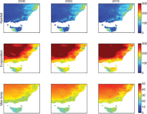
|
Water chemistry
As a result of the changes to freshwater systems discussed in the sections above, several additional changes may occur to the chemistry of inland waters, including pH, salinity and nutrient dynamics. Potential future changes in these properties cannot be obtained directly from climate models for individual water bodies in Australia; however, some general trends are anticipated on the basis of the projected changes in temperature and rainfall. Catchment and watershed models can likely be enhanced to allow local scenarios of future change to be investigated for inland waters (Ficke et al. 2007; Post et al. 2007) and partnership with modellers will be particularly important for freshwater fish biologists assessing future impacts.
Like marine waters, dissolution of CO2 in freshwater will lead to changes in pH. In natural freshwater bodies, pH generally varies between 6.5 and 8, and dissolution of additional CO2 will lead to pH declining, just as for oceanic systems. The pH of inland waters can also change as a result of changes in soil chemistry. If sulfidic sediments are present in the soils or wetland margins, drying can result in oxidisation of the sulfidic minerals and generate acid sulfate soils (Hall et al. 2006; Baldwin et al. 2007). This may be a common problem in some parts of Australia. For example, more than 20% of 81 wetlands in the Murray–Darling Basin had sulfidic sediments at levels that could lead to ecological damage (Hall et al. 2006). Oxidation of sulfidic sediments can also cause other problems such as anoxia in the overlying water column and mobilisation of metals from the sediments (see Baldwin et al. 2007). Thus, increased drying as a result of climate change, followed by flooding or rewetting may lead to major changes in water chemistry (depleted oxygen, very low pH), resulting in fish kills. Water managers should consider this potential when managing (Baldwin et al. 2007) or restoring (Hall et al. 2006) water bodies adjacent to acid sulfate soils, because the drying trends projected for the Murray–Darling and south-western Australia will exacerbate the existing problems.
Reduced runoff and increased drying in some areas have elevated salinity levels (e.g. south-western Australia). Some inland ‘freshwater’ habitats in Australia are already considered hypersaline (e.g. Lake Eyre basin) and the fauna that inhabit them possess characteristics that promote tolerance of such extreme environments (see discussion in Morrongiello et al. 2011). However, critical thresholds for most species are unknown. Reduced ‘average’ runoff followed by intense flooding or bushfires may also increase sedimentation input (Steffen 2009). If fertiliser inputs to land continue, reduced average flows followed by extreme flooding could also lead to increased nutrient load that arrives all at once (i.e. large single input v. small continuous inputs). Catchment models at a watershed scale could be used to generate future scenarios of nutrient loads (e.g. Post et al. 2007) and these projections would be useful to biologists and water-resource managers.
Extreme events
Climate change is intensifying the global hydrological cycle, with water being cycled more rapidly between atmosphere and ocean (Held and Soden 2006). As a result, more intense storms are projected to occur, although this is an area of considerable debate amongst scientists, even for the historical record (e.g. Graham and Diaz 2001; Emanuel 2005). In the Australian region, there is evidence for a decline in the frequency of tropical cyclones (see Lough and Hobday 2011; http://www.bom.gov.au/cyclone/climatology/trends.shtml, accessed 24 August 2011). Some climate models project that although there maybe fewer tropical cyclones in the future, those that do occur may be of higher intensity (IPCC 2007). Increased wind speed has also been detected in some climate models; however, future projections regarding extreme events must be viewed cautiously at this time. Accepting this caveat, increases in storm intensity have been coupled with sea-level trends to model coastal impacts. For example, McInnes et al. (2003) used a RCM for Cairns in north-eastern Australia, and showed that projected increases in cyclone intensity based on a doubling of CO2 by 2050 can result in a storm-surge event with a return period of 100 years, becoming a 55-year event by 2050 and a 40-year event when sea-level rise is included. On land, greater fire frequency and intensity could contaminate water catchments with sediment and ash, and floods may be more intense if projections of increased storm intensity are correct (Steffen 2009). With regard to future impacts, an important area of research for biologists is to determine the relative influence of extreme events versus long-term gradual changes in environmental conditions in driving population responses.
Prospects for Australian aquatic ecosystems
Changes in the physical environment of aquatic ecosystems have already been observed around Australia (Lough and Hobday 2011), and the rate of change is likely to increase with ongoing climate change. Drastic cuts in global greenhouse-gas emissions are necessary to curtail the impact of future change, and prevent devastating effects of extreme climate change. However, inertia in the climate system will lead to ongoing warming and sea-level rise throughout the 21st century, even if emissions stop today. The projections for Australian marine systems show higher temperatures, rising sea level and lower pH in the coming years, whereas for freshwater systems, inferences based on declining rainfall in many parts of the country suggest that stream flow and lake levels will also decline in these locations.
To improve performance of GCMs and the use of GCM-based projections, improved resolution of mesoscale processes is critical. One way to achieve this is to link RCMs with GCMs to project impacts at a regional scale (e.g. Hartog et al. 2011). A challenge given the computing time this involves is to generate a suitable suite of scenario–model combinations so that future conditions and the associated uncertainty can be assessed. To improve confidence in model-based projections, historical validation is important (Smith and Chandler 2010). In the case of Australia, this means a commitment to maintaining critical in situ ocean-climate observations, now realised under the IMOS program (www.imos.org.au, accessed 24 August 2011). These provide important verification for longer-term but less spatially detailed datasets, ground-truthing of satellite observations and linking the physical and biological components of the marine environment at scales relevant to the physiological processes of marine organisms (Lough 2009; Lough et al. 2010). Equally important is to continue to maintain high-quality remote sensing for Australian waters. Integration of both in situ and remote-sensed products with longer-term datasets will be valuable to many users.
Whereas the present paper has focussed on the use of climate projections in biological application, improved understanding of the biota, community and ecosystem is essential to credibly translate the climate projection into biological impacts. For many impacts, such as ocean acidification, a lack of biological information is limiting our ability to project future biological impacts. Experimental studies may help address this concern and help in parameterising impact models.
A critical question for aquatic biologists working on climate-change impacts centres on the adaptation potential of affected species and habitats. Vulnerability assessments (e.g. Hobday et al. 2007; Johnson and Marshall 2007) rely on estimates of present or future exposure to climate change to determine species or habitat vulnerability. Similarly, information on future physical changes is a pre-requisite to more detailed study of biological impacts, such as quantitative population models (e.g. Wolf et al. 2010). These more detailed biological models are necessary to consider the effect of adaptation options, and tradeoffs between competing human needs. With improved physical information on historical and future trends, and awareness of how to use the available information, the impacts of climate change for Australian aquatic environments can be better predicted, and effective and cost-efficient adaptation options implemented to ‘manage the avoidable’, while continuing to implement mitigation efforts to ‘avoid the unmanageable’ (SEG 2007).
Acknowledgements
The support of the Australian Society of Fish Biology at the 2010 Climate Change Symposium is gratefully acknowledged, together with the support of the coordinator of the Symposium and lead editor of this Special Issue, John Koehn. Acidification projections were generated by Richard Matear who was supported in-part by the Pacific Climate Change Science Program for his contribution to the SPC volume Pacific Fisheries and Climate Change: A Vulnerability Assessment. Tom Harwood graciously supplied the downscaled projections for rainfall. We appreciate the comments by three reviewers, guest editors John Koehn and Morgan Pratchett, and chief editor Andrew Boulton, that improved the clarity and coverage of the discussion.
References
Anthony, K. R. N., Kline, D. I., Diaz-Pulido, G., Dove, S., and Hoegh-Guldberg, O. (2008). Ocean acidification causes bleaching and productivity loss in coral reef builders. Proceedings of the National Academy of Sciences, USA 105, 17442–17446.| Ocean acidification causes bleaching and productivity loss in coral reef builders.Crossref | GoogleScholarGoogle Scholar | 1:CAS:528:DC%2BD1cXhsVWns7jM&md5=9813e98d93b7d56631ca0219fc3e283fCAS |
Baldwin, D. S., Hall, K. C., Rees, G. N., and Richardson, A. J. (2007). Development of a protocol for recognizing sulfidic sediments (potential acid sulfate soils) in freshwater wetlands. Ecological Management Restoration 8, 56–60.
| Development of a protocol for recognizing sulfidic sediments (potential acid sulfate soils) in freshwater wetlands.Crossref | GoogleScholarGoogle Scholar |
Byrne, M., Ho, M., Selvakumaraswamy, P., Ngyuen, H. D., Dworjanyn, S. A., and Davis, A. R. (2009). Temperature, but not pH, compromises sea urchin fertilization and early development under near-future climate change scenarios. Proceedings of the Royal Society of London. Series B. Biological Sciences 276, 1883–1888.
| Temperature, but not pH, compromises sea urchin fertilization and early development under near-future climate change scenarios.Crossref | GoogleScholarGoogle Scholar |
Cai, W. (2006). Antarctic ozone depletion causes an intensification of the Southern Ocean supergyre circulation. Geophysical Research Letters 33, L03712.
| Antarctic ozone depletion causes an intensification of the Southern Ocean supergyre circulation.Crossref | GoogleScholarGoogle Scholar |
Cai, W., and Cowan, T. (2008a). Dynamics of late autumn rainfall reduction over southeastern Australia. Geophysical Research Letters 35, L09708.
| Dynamics of late autumn rainfall reduction over southeastern Australia.Crossref | GoogleScholarGoogle Scholar |
Cai, W., and Cowan, T. (2008b). Evidence of impacts from rising temperatures on inflows to the Murray–Darling Basin. Geophysical Research Letters 35, L07701.
| Evidence of impacts from rising temperatures on inflows to the Murray–Darling Basin.Crossref | GoogleScholarGoogle Scholar |
Cai, W., Shi, G., Cowan, T., Bi, D., and Ribbe, J. (2005). The response of the Southern Annular Mode, the East Australian Current, and the southern mid-latitude ocean circulation to global warming. Geophysical Research Letters 32, L23706.
| The response of the Southern Annular Mode, the East Australian Current, and the southern mid-latitude ocean circulation to global warming.Crossref | GoogleScholarGoogle Scholar |
Chiew, F. H. S., Teng, J., Kirono, D., Frost, A. J., Bathols, J. M., Vaze, J., Viney, N. R., Young, W. J., Hennessy, K. J., and Cai, W. J. (2008). Climate data for hydrologic scenario modelling across the Murray–Darling Basin. A report to the Australian Government from the CSIRO Murray–Darling Basin Sustainable Yields Project. CSIRO, Australia. Available at http://www.csiro.edu.au/files/files/plok.pdf [verified 2 June 2011].
Church, J. A., White, N. J., Hunter, J. R., McInnes, K., and Mitchell, W. (2009). Sea level. In ‘A Marine Climate Change Impacts and Adaptation Report Card for Australia 2009’. (Eds E. S. Poloczanska, A. J. Hobday and A. J. Richardson.) NCCARF Publication 05/09, ISBN 978-1-921609-03-9. Available at www.oceanclimatechange.org.au [verified 2 June 2011].
CSIRO (2007). ‘Climate Change in Australia.’ Available at http://www.climatechangeinaustralia.gov.au/ [verified 2 June 2011].
De’ath, G., Lough, J. M., and Fabricius, K. E. (2009). Declining coral calcification on the Great Barrier Reef. Science 323, 116–119.
| Declining coral calcification on the Great Barrier Reef.Crossref | GoogleScholarGoogle Scholar | 1:CAS:528:DC%2BD1MXovF2i&md5=6b268d4617c2df24e1bc46831e850a35CAS |
Deo, R. C., Syktus, J. I., McAlpine, C. A., Lawrence, P. J., McGowan, H. A., and Phinn, S. R. (2009). Impact of historical land cover change on daily indices of climate extremes including droughts in eastern Australia. Geophysical Research Letters 36, L08705.
| Impact of historical land cover change on daily indices of climate extremes including droughts in eastern Australia.Crossref | GoogleScholarGoogle Scholar |
Doney, S. C., Fabry, V. J., Feely, R. A., and Kleypas, J. A. (2009). Ocean acidification: the other CO2 problem. Annual Review of Marine Science 1, 169–192.
| Ocean acidification: the other CO2 problem.Crossref | GoogleScholarGoogle Scholar |
Emanuel, K. A. (2005). Increasing destructiveness of tropical cyclones over the past 30 years. Nature 436, 686–688.
| Increasing destructiveness of tropical cyclones over the past 30 years.Crossref | GoogleScholarGoogle Scholar | 1:CAS:528:DC%2BD2MXmvFenurY%3D&md5=6a7646157adf2ea8a6b1246f29c124bbCAS |
Feng, M., Weller, E., and Hill, K. (2009). The Leeuwin Current. In ‘A Marine Climate Change Impacts and Adaptation Report Card for Australia 2009’. (Eds E. S. Poloczanska, A. J. Hobday and A. J. Richardson) NCCARF Publication 05/09, ISBN 978-1-921609-03-9. Available at www.oceanclimatechange.org.au [verified 2 June 2011].
Ficke, A. D., Myrick, C. A., and Hansen, L. J. (2007). Potential impacts of global climate change on freshwater fisheries. Reviews in Fish Biology and Fisheries 17, 581–613.
| Potential impacts of global climate change on freshwater fisheries.Crossref | GoogleScholarGoogle Scholar |
Figueira, W. F., and Booth, D. J. (2010). Increasing ocean temperatures allow tropical fishes to survive overwinter in temperate waters. Global Change Biology 16, 506–516.
| Increasing ocean temperatures allow tropical fishes to survive overwinter in temperate waters.Crossref | GoogleScholarGoogle Scholar |
Gillanders, B. M., Elsdon, T. S., Halliday, I. A., Jenkins, G. P., Robins, J. B., and Valesini, F. J. (2011). Potential effects of climate change on Australian estuaries and fish-utilising estuaries: a review. Marine and Freshwater Research 62, 1115–1131.
| Potential effects of climate change on Australian estuaries and fish-utilising estuaries: a review.Crossref | GoogleScholarGoogle Scholar |
Gillett, N. P., and Thompson, D. W. J. (2003). Simulation of recent southern hemisphere climate change. Science 302, 273–275.
| Simulation of recent southern hemisphere climate change.Crossref | GoogleScholarGoogle Scholar | 1:CAS:528:DC%2BD3sXnvFWgtLw%3D&md5=e811abb2f73a554ce9d005e85055bc7bCAS |
Graham, N. E., and Diaz, H. F. (2001). Evidence for intensification of North Pacific winter cyclones since 1948. Bulletin of the American Meteorological Society 82, 1869–1893.
| Evidence for intensification of North Pacific winter cyclones since 1948.Crossref | GoogleScholarGoogle Scholar |
Hall, K. C., Baldwin, D. S., Rees, G. N., and Richardson, A. J. (2006). Distribution of inland wetlands with sulfidic sediments in the Murray–Darling Basin, Australia. The Science of the Total Environment 370, 235–244.
| Distribution of inland wetlands with sulfidic sediments in the Murray–Darling Basin, Australia.Crossref | GoogleScholarGoogle Scholar | 1:CAS:528:DC%2BD28XpvF2ns70%3D&md5=e7911dd5419d8641675f320704249532CAS |
Hartog, J. R., Hobday, A. J., Matear, R., and Feng, M. (2011). Habitat overlap between southern bluefin tuna and yellowfin tuna in the east coast longline fishery – implications for present and future spatial management. Deep Sea Research Part II 58, 746–752.
| Habitat overlap between southern bluefin tuna and yellowfin tuna in the east coast longline fishery – implications for present and future spatial management.Crossref | GoogleScholarGoogle Scholar |
Harwood, T., Williams, K. J., and Ferrier, S. (2010). Generation of spatially downscaled climate change predictions for Australia. A report to the Department of Environment, Water, Heritage and the Arts, CSIRO, Canberra.
Held, I. M., and Soden, B. J. (2006). Robust responses of the hydrological cycle to global warming. Journal of Climate 19, 5686–5699.
| Robust responses of the hydrological cycle to global warming.Crossref | GoogleScholarGoogle Scholar |
Hennessy, K., Fitzharris, B., Bates, B. C., Harvey, N., Howden, M., Hughes, L., Salinger, J., and Warrick, R. (2007). Australia and New Zealand. In ‘Climate Change 2007: Impacts, Adaptation and Vulnerability. Contribution of Working Group II to the Fourth Assessment Report of the Intergovernmental Panel on Climate Change’. (Eds M. L. Parry, O. F. Canziani, J. P. Palutikof, C. E. Hanson and P. van der Linden.) pp. 506–540. (Cambridge University Press: Cambridge, UK.)
Hobday, A. J. (2010). Ensemble analysis of the future distribution of large pelagic fishes in Australia. Progress in Oceanography 86, 291–301.
| Ensemble analysis of the future distribution of large pelagic fishes in Australia.Crossref | GoogleScholarGoogle Scholar |
Hobday, A. J., Okey, T. A., Poloczanska, E. S., Kunz, T. J., and Richardson, A. J. (2007). Impacts of climate change on Australian marine life. CSIRO Marine and Atmospheric Research. Report to the Australian Greenhouse Office, Canberra. Available at http://www.cmar.csiro.au/climateimpacts/reports.htm
Hoegh-Guldberg, O., Mumby, P. J., Hooten, A. J., Steneck, R. S., Greenfield, P., Gomez, E., Harvell, C. D., Sale, P. F., Edwards, A. J., Caldeira, K., Knowlton, N., Eakin, C. M., Iglesias-Prieto, R., Muthiga, N., Bradbury, R. H., Dubi, A., and Hatziolos, M. E. (2007). Coral reefs under rapid climate change and ocean acidification. Science 318, 1737–1742.
| Coral reefs under rapid climate change and ocean acidification.Crossref | GoogleScholarGoogle Scholar | 1:CAS:528:DC%2BD2sXhsVWhu7fN&md5=b074c829a513c1a5f7a4dd1596f39ea3CAS |
Howard, W. R., Havenhand, J., Parker, L., Raftos, D., Ross, P., Williamson, J., and Matear, R. (2009). Ocean acidification. In ‘A Marine Climate Change Impacts and Adaptation Report Card for Australia 2009’. (Eds E. S. Poloczanska, A. J. Hobday and A. J. Richardson) NCCARF Publication 05/09, ISBN 978-1-921609-03-9. Available at www.oceanclimatechange.org.au [verified 2 June 2011].
Hughes, L. (2003). Climate change and Australia: trends, projections and impacts. Austral Ecology 28, 423–443.
| Climate change and Australia: trends, projections and impacts.Crossref | GoogleScholarGoogle Scholar |
Hulme, P. E. (2005). Adapting to climate change: is there scope for ecological management in the face of a global threat? Journal of Applied Ecology 42, 784–794.
| Adapting to climate change: is there scope for ecological management in the face of a global threat?Crossref | GoogleScholarGoogle Scholar |
IPCC (2007). Summary for policymakers. In ‘Climate Change 2007: Impacts, Adaptation and Vulnerability. Contribution of Working Group II to the Fourth Assessment Report of the Intergovernmental Panel on Climate Change’. (Eds M. L. Parry, O. F. Canziani, J. P. Palutikof, P. J. van der Linden and C. E. Hanson.) pp. 7–22. (Cambridge University Press: Cambridge, UK.)
Johnson, J. E., and Marshall, P. A. (Eds) (2007). Climate change and the Great Barrier Reef. Great Barrier Reef Marine Park Authority and Australian Greenhouse Office. Available at http://www.gbrmpa.gov.au/__data/assets/pdf_file/0007/22588/01-preliminary-pages.pdf [verified 2 June 2011].
Last, P. R., White, W. T., Gledhill, D. C., Hobday, A. J., Brown, R., Edgar, G. J., and Pecl, G. (2011). Long-term shifts in abundance and distribution of a temperate fish fauna: a response to climate change and fishing practices. Global Ecology and Biogeography 20, 58–72.
| Long-term shifts in abundance and distribution of a temperate fish fauna: a response to climate change and fishing practices.Crossref | GoogleScholarGoogle Scholar |
Le Quéré, C., Raupach, M. R., Canadell, J. G., Marland, G., Bopp, L., Ciais, P., Conway, T. J., Doney, S. C., Feely, R. A., Foster, P., Friedlingstein, P., Gurney, K., Houghton, R. A., House, J. I., Huntingford, C., Levy, P. E., Lomas, M. R., Majkut, J., Metzl, N., Ometto, J. P., Peters, G. P., Prentice, I. C., Randerson, J. T., Running, S. W., Sarmiento, J. L., Schuster, U., Sitch, S., Takahashi, T., Viovy, N., van der Werf, G. R., and Woodward, F. I. (2009). Trends in the sources and sinks of carbon dioxide. Nature Geoscience 2, 831–836.
| Trends in the sources and sinks of carbon dioxide.Crossref | GoogleScholarGoogle Scholar |
Lough, J. M. (2008). Shifting climate zones for Australia’s tropical marine ecosystems. Geophysical Research Letters 35, L14708.
| Shifting climate zones for Australia’s tropical marine ecosystems.Crossref | GoogleScholarGoogle Scholar |
Lough, J. M. (2009). Temperature. In ‘A Marine Climate Change Impacts and Adaptation Report Card for Australia 2009’. (Eds E. S. Poloczanska, A. J. Hobday and A. J. Richardson.) NCCARF Publication 05/09, ISBN 978-1-921609-03-9. Available at www.oceanclimatechange.org.au [verified 2 June 2011].
Lough, J. M., and Hobday, A. J. (2011). Observed climate change in Australian marine and freshwater environments. Marine and Freshwater Research 62, 984–999.
| Observed climate change in Australian marine and freshwater environments.Crossref | GoogleScholarGoogle Scholar |
Lough, J., Bainbridge, S., Berkelmans, R., and Steinberg, C. (2010). Physical monitoring of the Great Barrier Reef to understand ecological responses to climate change. In ‘Climate Alert: Climate Change Monitoring and Strategy’. (Eds Y. Yuzhu and A. Henderson-Sellers.) pp. 66–110. (University of Sydney Press: University of Sydney.)
Marti, O., Braconnot, P., Dufresne, J.-L., Bellier, J., Benshila, R., Bony, S., Brockmann, P., Cadule, P., Caudel, A., Codron, F., de Noblet, N., Denvil, S., Fairhead, L., Fichefet, T., Foujols, M.-A., Friedlingstein, P., Goosse, H., Grandpeix, J.-Y., Guilyardi, E., Hourdin, F., Idelkadi, A., Kageyama, M., Krinner, G., Lévy, C., Madec, G., Mignot, J., Musat, I., Swingedouw, D., and Talandier, C. (2010). Key features of the IPSL ocean atmosphere model and its sensitivity to atmospheric resolution. Climate Dynamics 34, 1–26.
| Key features of the IPSL ocean atmosphere model and its sensitivity to atmospheric resolution.Crossref | GoogleScholarGoogle Scholar |
McInnes, K. L., Walsh, K. J. E., Hubbert, G. D., and Beer, T. (2003). Impact of sea-level rise and storm surges on a coastal community. Natural Hazards 30, 187–207.
| Impact of sea-level rise and storm surges on a coastal community.Crossref | GoogleScholarGoogle Scholar |
McNeil, B. I., and Matear, R. J. (2008). Southern Ocean acidification: a tipping point at 450-ppm atmospheric CO2. Proceedings of the National Academy of Sciences, USA 105, 18860–18864.
| Southern Ocean acidification: a tipping point at 450-ppm atmospheric CO2.Crossref | GoogleScholarGoogle Scholar | 1:CAS:528:DC%2BD1cXhsV2rtL3E&md5=1ad091d68b084aecc8e1e9eb83e4b872CAS |
Morrongiello, J. R., Beatty, S. J., Bennett, J. C., Crook, D. A., Ikedife, D. N. E. N., Kennard, M. J., Kerezsy, A., Lintermans, M., McNeil, D. G., Pusey, B. J., and Rayner, T. (2011). Climate change and its implications for Australia’s freshwater fish. Marine and Freshwater Research 62, 1082–1098.
| Climate change and its implications for Australia’s freshwater fish.Crossref | GoogleScholarGoogle Scholar |
Moss, R. H., Edmonds, J. A., Hibbard, K. A., Manning, M. R., Rose, S. K., van Vuuren, D. P., Carter, T. R., Emori, S., Kainuma, M., Kram, T., Meehl, G. A., Mitchel, J. F. B., Nakicenovic, N., Riahi, K., Smith, S. J., Stouffer, R. J., Thomson, A. M., Weyant, J. P., and Wilbanks, T. J. (2010). The next generation of scenarios for climate change research and assessment. Nature 463, 747–756.
| The next generation of scenarios for climate change research and assessment.Crossref | GoogleScholarGoogle Scholar | 1:CAS:528:DC%2BC3cXhvVKqs7w%3D&md5=4695ffc4d8a122b482b24da99ae49afaCAS |
Munday, P. L., Donelson, J. M., Dixson, D. L., and Endo, G. G. K. (2009). Effects of ocean acidification on the early life history of a tropical marine fish. Proceedings of the National Academy of Sciences, USA 276, 3275–3283.
| 1:CAS:528:DC%2BD1MXhtFCgsLrJ&md5=39f3ac5437e108caa78e0f735a3df105CAS |
Oke, P. R., Brassington, G. B., Griffin, D. A., and Schiller, A. (2008). The Bluelink ocean data assimilation system (BODAS). Ocean Modelling 21, 46–70.
| The Bluelink ocean data assimilation system (BODAS).Crossref | GoogleScholarGoogle Scholar |
Orr, J. C., Fabry, V. J., Aumont, O., Bopp, L., Doney, S. C., Feely, R. A., Gnanadesikan, A., Gruber, N., Ishida, A., Joos, F., Key, R. M., Lindsay, K., Maier-Reimer, E., Matear, R., Monfray, P., Mouchet, A., Najjar, R. G., Plattner, G.-K., Rodgers, K. B., Sabine, C. L., Sarmiento, J. L., Schlitzer, R., Slater, R. D., Totterdell, I. J., Weirig, M.-F., Yamanaka, Y., and Yool, A. (2005). Anthropogenic ocean acidification over the twenty-first century and its impact on calcifying organisms. Nature 437, 681–686.
| Anthropogenic ocean acidification over the twenty-first century and its impact on calcifying organisms.Crossref | GoogleScholarGoogle Scholar | 1:CAS:528:DC%2BD2MXhtVCjsL%2FE&md5=9390bc0fada8743ec20f80a7ffe47e99CAS |
Pankhurst, N. W., and Munday, P. L. (2011). Effects of climate change on fish reproduction and early life history stages. Marine and Freshwater Research 62, 1015–1026.
| Effects of climate change on fish reproduction and early life history stages.Crossref | GoogleScholarGoogle Scholar |
Pearce, A., and Feng, M. (2007). Observations of warming on the Western Australian continental shelf. Marine and Freshwater Research 58, 914–920.
| Observations of warming on the Western Australian continental shelf.Crossref | GoogleScholarGoogle Scholar |
Perkins, S. E., Pitman, A. J., and Sisson, S. A. (2009). Smaller projected increases in 20-year temperature returns over Australia in skill-selected climate models. Geophysical Research Letters 36, L06710.
| Smaller projected increases in 20-year temperature returns over Australia in skill-selected climate models.Crossref | GoogleScholarGoogle Scholar |
Pierce, D. W., Barnett, T. P., Santer, B. D., and Gleckler, P. J. (2009). Selecting global climate models for regional climate change studies. Proceedings of the National Academy of Sciences, USA 106, 8441–8446.
| 1:CAS:528:DC%2BD1MXnt1Sru74%3D&md5=43cbc0c515914d144e7e973959a2878cCAS |
Poloczanska, E. S., Babcock, R. C., Butler, A., Hobday, A. J., Hoegh-Guldberg, O., Kunz, T. J., Matear, R., Milton, D., Okey, T. A., and Richardson, A. J. (2007). Climate change and Australian marine life. Oceanography and Marine Biology Annual Review 45, 409–480.
Poloczanska, E. S., Hobday, A. J., and Richardson, A. J. (Eds) (2009). ‘A Marine Climate Change Impacts and Adaptation Report Card for Australia 2009.’ NCCARF Publication 05/09, ISBN 978-1-921609-03-9. Available at www.oceanclimatechange.org.au [verified 2 June 2011].
Post, D. A., Waterhouse, J., Grundy, M., and Cook, F. (2007). The past, present and future of sediment and nutrient modelling in GBR Catchments. CSIRO, Water for a Healthy Country National Research Flagship. Available at http://www.csiro.au/files/files/pg8j.pdf [verified 4 June 2011].
Pratchett, M. S., Bay, L. K., Gehrke, P. C., Koehn, J. D., Osborne, K., Pressey, R. L., Sweatman, H. P. A., and Wachenfeld, D. (2011). Contribution of climate change to degradation and loss of critical fish habitats in Australian marine and freshwater environments. Marine and Freshwater Research 62, 1062–1081.
| Contribution of climate change to degradation and loss of critical fish habitats in Australian marine and freshwater environments.Crossref | GoogleScholarGoogle Scholar |
Przeslawski, R., Ayhong, S., Byrne, M., Worheides, G., and Hutchings, P. (2008). Beyond corals and fish: the effects of climate change on noncoral benthic invertebrates of tropical reefs. Global Change Biology 14, 2773–2795.
| Beyond corals and fish: the effects of climate change on noncoral benthic invertebrates of tropical reefs.Crossref | GoogleScholarGoogle Scholar |
Rahmstorf, S., Cazenave, A., Church, J. A., Hansen, J. E., Keeling, R. F., Parker, D. E., and Somerville, R. C. J. (2007). Recent climate observations compared to projections. Science 316, 709.
| Recent climate observations compared to projections.Crossref | GoogleScholarGoogle Scholar | 1:CAS:528:DC%2BD2sXkvVWrsL4%3D&md5=85b1287a6ff44da3695e07c14773f0d9CAS |
Ridgway, K. R. (2007). Long-term trend and decadal variability of the southward penetration of the East Australian Current. Geophysical Research Letters 34, L13613.
| Long-term trend and decadal variability of the southward penetration of the East Australian Current.Crossref | GoogleScholarGoogle Scholar |
Schmidli, J., Frei, C., and Vidale, P. L. (2006). Downscaling from GCM precipitation: a benchmark for dynamical and statistical downscaling methods. International Journal of Climatology 26, 679–689.
| Downscaling from GCM precipitation: a benchmark for dynamical and statistical downscaling methods.Crossref | GoogleScholarGoogle Scholar |
Schneider, S. H. (2009). The worst-case scenario. Nature 458, 1104–1105.
| The worst-case scenario.Crossref | GoogleScholarGoogle Scholar | 1:CAS:528:DC%2BD1MXlt1Srsbo%3D&md5=ac4aeb3cc64775f09474c1933d82bb70CAS |
Scientific Expert Group on Climate Change (SEG) (2007). ‘Confronting Climate Change: Avoiding the Unmanageable and Managing the Unavoidable.’ (Eds R. M. Bierbaum, J. P. Holdren, M. C. McCracken, R. H. Moss and P. H. Raven). Report prepared for the United Nations Commission on Sustainable Development, Sigma Xi, Research Triangle Park, NC and the United Nations Foundation, Washington DC. Available at http://www.globalproblems-globalsolutions-files.org/unf_website/PDF/climate%20_change_avoid_unmanagable_manage_unavoidable.pdf [verified 2 June 2011].
Sheppard Brennand, H., Soars, N., Dworjanyn, S. A., Davis, A. R., and Byrne, M. (2010). Impact of ocean warming and ocean acidification on larval development and calcification in the sea urchin Tripneustes gratilla. PLoS ONE 5, e11372.
| Impact of ocean warming and ocean acidification on larval development and calcification in the sea urchin Tripneustes gratilla.Crossref | GoogleScholarGoogle Scholar |
Shukla, J., Hagedorn, R., Miller, M., Palmer, T. N., Hoskins, B., Kinter, J., Marotzke, J., and Slingo, J. (2009). Revolution in climate prediction is both necessary and possible: a declaration at the world modelling summit for climate prediction. Bulletin of the American Meteorological Society 90, 175–178.
| Revolution in climate prediction is both necessary and possible: a declaration at the world modelling summit for climate prediction.Crossref | GoogleScholarGoogle Scholar |
Smith, I., and Chandler, E. (2010). Refining rainfall projections for the Murray Darling Basin of south-east Australia – the effect of sampling model results based on performance. Climatic Change 102, 377–393.
| Refining rainfall projections for the Murray Darling Basin of south-east Australia – the effect of sampling model results based on performance.Crossref | GoogleScholarGoogle Scholar |
Solomon, S., Plattner, G.-K., Knutti, R., and Friedlingstein, P. (2009). Irreversible climate change due to carbon dioxide emissions. Proceedings of the National Academy of Sciences, USA 106, 1704–1709.
| Irreversible climate change due to carbon dioxide emissions.Crossref | GoogleScholarGoogle Scholar | 1:CAS:528:DC%2BD1MXitV2jur8%3D&md5=55425a31bc164def14d5b65131dfa96aCAS |
State of the Climate (2010). An update from CSIRO and the BOM. Available at www.bom.gov.au/inside/eiab/State-of-climate-2010-updated.pdf [verified 2 June 2011].
Steffen, W. (2009). ‘Climatic Change 2009. Faster Change and More Serious Risks.’ (Department of Climate Change, Commonwealth of Australia: Canberra. Australia.) Available at http://www.climatechange.gov.au/publications/science/faster-change-more-risk.aspx [verified 25 August 2011].
Stute, M., Clement, A., and Lohmann, G. (2001). Global climate models: past, present, and future. Proceedings of the National Academy of Sciences, USA 98, 10529–10530.
| Global climate models: past, present, and future.Crossref | GoogleScholarGoogle Scholar | 1:CAS:528:DC%2BD3MXntVGntbo%3D&md5=5aba4e236a56c14d2c753149591a8123CAS |
Suppiah, R., Hennessy, K. J., Whetton, P. H., McInnes, K., Macadam, I., Bathols, J., Ricketts, J., and Page, C. M. (2007). Australian climate change projections derived from simulations performed for the IPCC 4th Assessment Report. Australian Meteorological Magazine 56, 131–152.
Tabor, K., and Williams, J. W. (2010). Globally downscaled climate projections for assessing the conservation impacts of climate change. Ecological Applications 20, 554–565.
| Globally downscaled climate projections for assessing the conservation impacts of climate change.Crossref | GoogleScholarGoogle Scholar |
Ummenhofer, C. C., England, M. H., McIntosh, P. C., Meyers, G. A., Pook, M. J., Risbey, J. S., Gupta, A. S., and Taschetto, A. S. (2009). What causes southeast Australia’s worst droughts? Geophysical Research Letters 36, L04706.
| What causes southeast Australia’s worst droughts?Crossref | GoogleScholarGoogle Scholar |
Vasiliades, L., Loukas, A., and Patsonas, G. (2009). Evaluation of a statistical downscaling procedure for the estimation of climate change impacts on droughts. Natural Hazards and Earth System Sciences 9, 879–894.
| Evaluation of a statistical downscaling procedure for the estimation of climate change impacts on droughts.Crossref | GoogleScholarGoogle Scholar |
Whetton, P. H., McInnes, K. L., Jones, R. N., Hennessy, K. J., Suppiah, R., Page, C. M., Bathols, J., and Durack, P. J. (2005). Australian climate change projections for impact assessment and policy application: a review. CSIRO Marine and Atmospheric Research Paper Number 001. December 2005. (CSIRO: Melbourne, Australia.)
Williams, J. W., Jackson, S. T., and Kutzbach, J. E. (2007). Projected distributions of novel and disappearing climates by 2100 AD. Proceedings of the National Academy of Sciences, USA 104, 5738–5742.
| Projected distributions of novel and disappearing climates by 2100 AD.Crossref | GoogleScholarGoogle Scholar | 1:CAS:528:DC%2BD2sXkt1Kgsb8%3D&md5=ea256d68c0fe2c91335af6db58acc714CAS |
Wolf, S. G., Snyder, M. A., Sydeman, W. J., Doak, D. F., and Croll, D. A. (2010). Predicting population consequences of ocean climate change for an ecosystem sentinel, the seabird Cassin’s auklet. Global Change Biology 16, 1923–1935.
| Predicting population consequences of ocean climate change for an ecosystem sentinel, the seabird Cassin’s auklet.Crossref | GoogleScholarGoogle Scholar |