

An investigation of genetic connectivity shines a light on the relative roles of isolation by distance and oceanic currents in three diadromous fish species
J. E. O’Dwyer A B D , N. Murphy A B , Z. Tonkin C , J. Lyon C , W. Koster C , D. Dawson C , F. Amtstaetter C and K. A. Harrisson A B C
A Department of Ecology, Environment & Evolution, La Trobe University, Bundoora, Vic. 3086, Australia.
B Research Centre for Future Landscapes, La Trobe University, Bundoora, Vic. 3086, Australia.
C Arthur Rylah Institute for Environmental Research, Department of Environment, Land, Water and Planning, 123 Brown Street, Heidelberg, Vic. 3084, Australia.
D Corresponding author. Email: 18088076@students.latrobe.edu.au
Marine and Freshwater Research - https://doi.org/10.1071/MF20323
Submitted: 3 November 2020 Accepted: 4 May 2021 Published online: 25 June 2021
Journal Compilation © CSIRO 2021 Open Access CC BY-NC
Abstract
Understanding connectivity is crucial for the effective conservation and management of biota. However, measuring connectivity directly is challenging and it is often inferred based on assumptions surrounding dispersal potential, such as environmental history and species life history traits. Genetic tools are often underutilised, yet can infer connectivity reliably. Here, we characterise and compare the genetic connectivity and genetic diversity of three diadromous Australian fish species: common galaxias (Galaxias maculatus), tupong (Pseudaphritis urvillii) and Australian grayling (Prototroctes maraena). For each species, we investigate the extent of genetic connectivity across a study region in south-eastern Australia (~700 km). We further determine the potential roles of contemporary ocean currents in shaping the patterns of genetic connectivity observed. Individuals across multiple rivers were sampled and >3000 single nucleotide polymorphisms were genotyped for each species. We found differences in genetic connectivity for the three species: common galaxias were highly connected, and Australian grayling and tupong exhibited patterns of isolation by distance. The degree of genetic connectivity for tupong and Australian grayling appeared unrelated to oceanic currents. This study indicates that the degree of connectivity for different diadromous species can vary greatly despite broadly similar life history strategies, highlighting the potential value of genetic tools for informing species-specific management plans.
Introduction
Connectivity is critical to species survival, but in many instances is compromised through human impacts (Noss et al. 2012; Haddad et al. 2015; Wilson et al. 2016). Demographic connectivity benefits relate to colonisation, population reestablishment and source and sink dynamics (Hanski 1998). Connectivity also has genetic benefits, buffering local populations against loss of genetic diversity by genetic drift, reducing inbreeding depression and promoting adaptive potential (Lowe and Allendorf 2010; Smith et al. 2014). Given its importance for species survival, conservation management practices are increasingly incorporating connectivity as a key component of long-term species management and recovery plans while actively considering the relative connectivity benefits from both a genetic and demographic perspective (Almany et al. 2009; Carroll et al. 2015; Magris et al. 2016).
What influences connectivity at a population level is often the result of complex interactions between present-day geography, the geographic history of a region, species biology and species-specific density-dependent processes, making population connectivity often highly specific to a species or area (Riginos et al. 2011; Waters et al. 2013). In many systems, large physical biogeographic barriers (e.g. land bridges, rivers and mountain ranges) can block or impede population connectivity, resulting in common patterns of population structure among diverse taxa (Pascual et al. 2017; Thacker 2017; Sánchez-Montes et al. 2018). Although physical barriers are easily observed, more subtle barriers can influence connectivity, such as resource and temperature differences in habitats limiting movement between populations by reducing the fitness of migrants arriving from different conditions (Friesen 2015). Population connectivity can also be influenced by life history traits, such as fecundity, size or either sessile or motile larval stages, which influence individual dispersal potential (Selkoe and Toonen 2011; Stevens et al. 2012; Whitmee and Orme 2013). Further, barriers and biological traits often interact, creating a relationship where stronger dispersers are less affected by barriers (Pascual et al. 2017). Ultimately, however, if the barriers to connectivity are sufficiently strong, even strong dispersers will lose population connectivity (Pascual et al. 2017). In addition to the interacting nature of barriers and biological traits, as species density increases many species have been shown to exhibit higher rates of dispersal and connectivity as a means of reducing overcrowding and resource limitations, further complicating the nature of species-level connectivity (Bitume et al. 2013, 2014).
Many studies have sought to predict connectivity based on the interactions between environment and species-specific biology (Bradbury et al. 2008; Stevens et al. 2014; Bonte and Dahirel 2017). These studies have helped identify many key factors influencing connectivity within individual species and groups of species that share similar life history traits (Stevens et al. 2014; Bonte and Dahirel 2017). However, these factors often fall short of adequately describing factors that universally influence connectivity across all scenarios (Clobert et al. 2012), highlighting the importance of species-specific connectivity studies to accurately infer population connectivity.
Riverine systems pose unique challenges to population connectivity for aquatic species. The highly linear and dendritic nature of rivers limits the connectivity of habitats and restricts the range of ways migrants can move, and therefore how populations can be connected (Jansson et al. 2007). These systems are additionally prone to complete isolation by natural barriers such as basin boundaries or human-induced barriers (e.g. dams, weirs) associated with river regulation (Puebla 2009; Birnie-Gauvin et al. 2017). In response to the more isolated and dendritic nature of freshwater habitats compared with more continuous oceanic habitats, many species have developed unique life history traits to promote connectivity, such as diadromy (McDowall 1999).
Diadromous species exhibit two distinct lifecycle stages, one in fresh water and one in the marine environment, with individuals migrating between the two environments to use resources or obtain connectivity benefits for a particular life stage (McDowall 1999). Among diadromous fishes, several specific modes of migration are recognised, including anadromy (mature adults migrate upstream from the sea to spawn in fresh water), catadromy (mature adults migrate from fresh water to spawn in the sea) and amphidromy (adults spawn in fresh water, with newly hatched larvae moving to the marine environment and returning to fresh water as juveniles; Myers 1949; McDowall 1988). Diadromous species typically show connectivity at a level intermediate to both freshwater and marine species due to their ability to use the highly connected marine environment for dispersal between otherwise isolated rivers (Ward et al. 1994). The degree of connectivity can vary greatly across diadromous species and is generally considered dependent on several life-history traits. Many life history traits have been shown to influence connectivity, with higher connectivity typically seen in diadromous species that show higher fecundities, larger body size or long-lasting pelagic larval stages, or those that actively disperse (Selkoe and Toonen 2011; Clobert et al. 2012; Feutry et al. 2013; Jones and Closs 2016). Although some economically important diadromous species such as salmonids have been studied extensively, diadromous species as a whole are a critically understudied group of fish, with many key questions surrounding how diadromy affects the overall connectivity seen within different diadromous species remaining (McDowall 1999; Delgado and Ruzzante 2020). This has ultimately resulted in insufficient knowledge of life history for many species to estimate dispersal.
Recent advances in genomic techniques have allowed for large-scale sequencing of genome-wide markers, producing thousands of markers compared with typical panels of 10–15 microsatellites traditionally used to measure genetic connectivity (Schmidt et al. 2011, 2014; Cook and Sgro 2017). With a larger number of genome-wide markers, more subtle patterns of connectivity can be resolved, allowing for finer-scale insights into population structure and connectivity. In addition, the use of large genomic datasets provides highly resolving information on important metrics of species viability, such as genetic diversity, effective population size and adaptive potential, helping highlight populations of conservation value and conservation concern (Cook and Sgro 2017).
In this study we used large-scale genomic datasets with thousands of single nucleotide polymorphic genetic markers to investigate patterns of genetic connectivity for three diadromous species: common galaxias (Galaxias maculatus), tupong (Pseudaphritis urvillii) and Australian grayling (Prototroctes maraena). These three species all use marine and freshwater environments and vary in several different life history traits commonly linked to dispersal, suggesting that connectivity may differ between the species (Miles 2007; Clobert et al. 2012). However, knowledge of the life history of each species is limited, with many key traits that can influence dispersal, such as larval mobility, unknown. Given such knowledge gaps surrounding key dispersal-linked life history traits, these species are ideal candidates for genomic-based assessments of connectivity. The aims of this study were to: (1) determine the extent of population genetic connectivity, levels of genetic diversity and effective population size estimates for each species; (2) investigate the role isolation by distance (IBD) and isolation by resistance (IBR) influenced by oceanic conditions play in population genetic connectivity for each species; and (3) determine whether differences in conservation status are reflected in the patterns of connectivity and genetic diversity observed for each species.
Materials and methods
Study species
The three study species exhibit differences in life history traits commonly linked to dispersal, including fecundity, larval size and movement strategies, and pelagic larval duration time, all of which may contribute to connectivity differences between each species (Table S1 of the Supplementary material). However, all species studied lack information on other key life history traits associated with larval dispersal, such as mobility, growth rates and preference for ocean depth. Further, many life history traits that are known for one species are not known for others, such as initial larval length and egg size (Table S1).
Common galaxias
Common galaxias G. maculatus is a widespread species with a distribution extending across Australia, New Zealand and South America (Gomon and Bray 2011). The form of diadromy exhibited by common galaxias is still debated, but is considered either amphidromous or semicatadromous, with adults migrating into estuaries to breed and larvae drifting into the marine environment before immigrating into rivers as juveniles (McDowall 2000; Bice et al. 2019b; Delgado and Ruzzante 2020). Adults produce thousands of eggs that hatch and undertake an ~5 month marine larval phase (McDowall et al. 1994). Otolith studies on New Zealand populations suggest high dispersal capabilities and population connectivity for the species along the New Zealand east and west coasts (Hickford and Schiel 2016). Genetic studies on populations along the Chilean coast show that the species exhibits very high diversity and connectivity (Delgado et al. 2019), but shows population genetic structuring at large spatial scales (>1000 km; Zemlak et al. 2010) as a result of past glacial events along the southern coast (González-Wevar et al. 2015). Its widespread distribution has led to common galaxias being classified as of least concern under International Union for Conservation of Nature (IUCN) status (Bice et al. 2019b).
Tupong
Tupong P. urvillii is a catadromous species endemic to the coastal drainages of south-east Australia (Gomon et al. 2008). Adults spawn during late autumn–winter in the sea (Crook et al. 2010), producing up to 400 000 eggs before juveniles enter rivers from the sea after approximately 4 months (Zampatti et al. 2010; Bice et al. 2012; Walker and Humphries 2013). Previous genetic work using microsatellite markers suggests tupong exhibit weak IBD structure (Schmidt et al. 2014). Its relative abundance through south and eastern Australia has led to tupong being classified as of least concern under IUCN status (Bice et al. 2019a).
Australian grayling
Australian grayling P. maraena is an amphidromous species. Adults mature and spawn in fresh water in autumn, producing up to 47 000 eggs, with the eggs and larvae drifting downstream to the sea and juveniles migrating back into fresh water after ~4–6 months (Berra 1982; Crook et al. 2006; Koster et al. 2013, 2021). Australian grayling has a similar distribution to tupong, but smaller estimated population sizes throughout Victoria (Allen et al. 2002), which, coupled with population declines, has led to Australian grayling being classified as a vulnerable species under the Environment Protection and Biodiversity Conservation Act 1999 of Australia and as vulnerable under IUCN status (Koster and Gilligan 2019). Previous genetic work analysing microsatellite and mitochondrial markers suggests that Australian grayling are connected between river populations around central and eastern Victoria (Schmidt et al. 2011).
Study region
Samples of each species were taken from rivers along the Victorian coast, south-east Australia (Fig. 1). The region contains two major oceanic currents, the East Australian Current (EAC), which flows south along the mainland eastern Australian coast towards Tasmania, and the South Australian Current (SAC), which flows eastward from the southern coast of Australia (Tilburg et al. 2001; Ridgway and Condie 2004). These currents vary seasonally, with the SAC flowing further into Bass Strait in winter and the EAC flowing further into Bass Strait during summer, creating a mosaic of directional flow depending on the season (Baird et al. 2006; Ridgway 2007).

|
Sample collection
Samples were collected from 94 common galaxias from 10 Victorian rivers (Table 1). Of these 94 individuals sampled, 69 were juveniles returning after their marine larval phase during Spring 2017 and 24 were from the same cohort sampled as young-of-the-year (YOY) during Autumn 2018 (Table 1). In addition, 94 tupong individuals were sampled from 7 rivers in Victoria. Of these 94 individuals, 28 were juveniles returning after their marine larval phase during the spring–summer of 2016 and 66 were from the same cohort sampled as YOY in February 2017 (Table 1). A total of 162 Australian grayling juveniles was sampled from 9 Victorian rivers and across three different year cohorts. Of these 162 individuals, 101 were juveniles collected after returning from their marine larval stage during the spring of 2016 and 27 were sampled from the same cohort as YOY collected in February 2017, 12 were collected as returning juveniles of a second-year cohort during the spring of 2018 and a further 22 were sampled as returning juveniles from a third-year cohort in the spring of 2019 (Table 1). All fin clips collected for common galaxias and tupong were part of the same cohort, but Australian grayling individuals were composed of two cohorts. All fin clips collected were stored in 95–100% ethanol and refrigerated at 4°C until later DNA extraction.
|
Sampling of individuals for this study was undertaken under the ethics permits AEC15/005 and AEC18/003 (ARI Animal Ethics Committee).
DNA extraction and sequencing
For common galaxias, ~5 mm2 of tissue was cut from the caudal or dorsal fins of each individual, and the tissue clips sent to Diversity Arrays Technology (DArT; Canberra, ACT, Australia), where total genomic DNA was extracted. For tupong and Australian grayling, DNA was extracted from small (~5 mm2) fin clips using a DNeasy Blood & Tissue kit (Qiagen) according to the manufacturer’s instructions. Approximately 20 µL of extracted DNA (at concentrations ranging from 5 to 20 ng µL–1) for each sample was sent to DArT for sequencing. The DNA was then sequenced using the Dartseq platform (Diversity Arrays Technology; www.diversityarrays.com). This platform uses a form of reduced representation sequencing similar to double-digest restriction site-associated DNA sequencing to generate large numbers of single nucleotide polymorphisms (SNPs). DNA samples were digested using two different enzymes, namely PstI and SphI, with two adaptors corresponding to the two different restriction enzyme overhangs, following the digestion and ligation methods described by Kilian et al. (2012). The forward (PstI) adaptor included an Illumina flow cell attachment sequence, sequencing primer sequence and a unique barcode for multiplexing, whereas the reverse adaptor included an Illumina flow cell attachment sequence. Only DNA fragments containing both cut sites were then amplified for sequencing because fragments that lacked one or both cut sites were unable to amplify. Equimolar amounts of each amplified product were then pooled and sequenced as single reads on an Illumina Hiseq 2500 for 77 cycles. Samples were sequenced in batches of 94 per Illumina sequencing lane, with 25% of samples rerun as technical replicates for quality control.
Data analysis
Sample and SNP filtering
Sequenced reads were processed using DArT proprietary analytical pipelines described in Kilian et al. (2012), with poor-quality sequences removed (based on the certainty of base calls and concordance with internal replicates run on a random subsample of 25% of individuals sequenced) and low-quality bases corrected using collapsed tags from multiple members as a template. A secondary pipeline (DArTsoft14) was then used to compile read counts into SNP loci calls with a maximum allowed difference between tags of three bases. SNPs were further filtered to remove loci whose allele read counts had a greater than fivefold difference from each other, and that scored <95% reproducibility using the sequenced technical replicates. Following the analytics pipelines, 58 997, 16 555 and 27 783 SNPs were genotyped for common galaxias, tupong and Australian grayling respectively.
SNPs processed using the DArT analytical pipelines were further filtered using the dartR package (ver. 1.1.11, CRAN.r, see https://CRAN.R-project.org/package=dartR; Gruber et al. 2018) in R (ver. 3.6.0, R Foundation for Statistical Computing, Vienna, Austria). All SNPs were filtered at a reproducibility value of 1, only retaining SNPs that were consistent in 100% of technical replicates sequenced as part of the Dartseq process (Table S3 of the Supplementary material). The data were filtered to remove any SNP that was missing in >10% of individuals, and only a single SNP per sequence tag was retained. All individuals were then filtered for a maximum allowable amount of missing data of 15%. All SNPs were then filtered to remove alleles that were present in <2% of all individuals from each species. After filtering, 8116 SNPs were retained for common galaxias, 6762 SNPs were retained for tupong, and 3410 SNPs were retained for Australian grayling.
Tests for Hardy–Weinberg equilibrium and neutrality
After filtering, all loci were investigated for Hardy–Weinberg equilibrium (HWE) using the dartR package in R. All markers were found to be in HWE for each species, and therefore no markers were removed at this stage.
Two methods were used to test for neutrality within the genetic markers used. The first method used was the fixation index (FST) outflank method implemented in the dartR package in R, whereas the second method used was through the program Bayescan (ver. 2.1, University of Bern, see http://www.cmpg.unibe.ch/software/BayeScan/; Foll and Gaggiotti 2008). For the FST outflank method, left and right trims of 5% of loci were used, and an α value of 0.05 Bonferroni corrected was used to identify putatively selected loci. For Bayescan, the Markov chain was run for 50 000 steps with a burn-in of 50 000 steps, a thinning interval of 10 and a total of 40 pilot runs composed of 10 000 steps. When plotting the results of Bayescan, a false discovery rate of 0.05 was used. Both methods identified zero loci for tupong and Australian grayling, and so no loci were filtered for either species before further analysis (Fig. S1–S5 in the ‘Neutrality tests of genetic markers’ section of the Supplementary material). Two loci were identified as putatively non-neutral for common galaxias, but were found along the border of significance (see the ‘Neutrality tests of genetic markers’ section of the Supplementary material). To test the impact of each locus, a subset of analyses was repeated without the two loci present. Because all analyses returned near identical results, the two loci were not filtered out (Tables S4–S7 and Fig. S1–S5 of the ‘Neutrality tests of genetic markers’ section of the Supplementary material).
Genetic diversity
Population genetic summary statistics including observed heterozygosity (Ho) expected heterozygosity (He) and allelic richness (AR) were calculated for each population and as species averages using the R software package hierfstat (ver. 0.04–22, CRAN.r, see https://cran.r-project.org/web/packages/hierfstat/index.html; Goudet 2005), and percentage polymorphic loci were calculated using custom code in R.
Kinship and potential dispersal events
Kinship analysis was used to identify sibling relationships between individuals, and therefore reveal connectivity patterns by identifying whether siblings were found to return to the same rivers or different rivers to each other, indicative of individual dispersal events. Further, identifying and removing sibling pairs can allow for increased accuracy when estimating population structure, dispersal and effective population sizes, because kinship can often mask true patterns of connectivity within datasets if unaccounted for (Peterman et al. 2016). Kinship analyses for each species were performed using the program Colony (ver. 2.0.6.5, Zoological Society of London, see https://www.zsl.org/science/software/colony; Jones and Wang 2010) to test for full-sibling and half-sibling pairs found across each species. Colony was run under the settings of combined pairwise and full-likelihood score (setting 2 out of 0–2), a genotyping error rate of 1%, updating allele frequencies (setting 1 out of 0/1), assumed polygamy for both males and females (setting 0 0 out of 0–1, 0–1), inbreeding, a long run (setting 3 out of 1–4) and for four runs that converged to average the most likely scenario. Using the results of these analyses, one individual from all full-sibling pairs was removed from each dataset for the analyses involving population structure, IBD, migration and oceanic resistance modelling.
Population genetic structure
To estimate the degree of population genetic structure among river populations within each species across the same geographic area, three different methods were used: (1) genetic differentiation (FST); (2) discriminate analysis of principal components (DAPC); and (3) and non-spatial clustering (Structure).
Pairwise FST values, which measure the degree of genetic differentiation between pairs of populations based on allele frequencies, were calculated using the R software package StAMPP (ver. 1.5.1, CRAN.r, https://cran.r-project.org/web/packages/StAMPP/index.html; Winter 2012). The significance of values was calculated using 100 000 bootstrap replicates of the data.
DAPC analyses were undertaken to estimate the number of genetic populations that exist within each species while also assigning individuals into their most likely genetic population. For DAPC, all individuals were assigned into optimal groups using successive K-means clustering from the find.clusters function in the R package adagenet (ver. 1.3.1, CRAN.r, see https://cran.r-project.org/web/packages/adegenet/index.html). For each species, K-means clustering suggested that in decreasing likelihood K = 1–4 were optimal based on the Bayesian inference criterion, so Clusters 1–4 were created.
Structure analysis was undertaken to complement DAPC, estimating the degree of spatial population genetic structure present in each species (Pritchard et al. 2000). For each species, Structure analysis was run with the number of genetic clusters (K) set from 1 to 10, with 14–17 (run time total of 50 CPU days per structure run) replicate runs of 200 000 Markov chain Monte Carlo iterations, after an initial burn-in period of 100 000 iterations. The results of each run were extracted using the program Structure Harvester (ver. 0.6.94, University of California, Los Angeles, CA, USA, see http://taylor0.biology.ucla.edu/structureHarvester/; Earl 2012), and the best fit for K was determined using both the Evanno method of a measure of the highest value of delta K (Evanno et al. 2005) and the highest overall likelihood of a structure output of fitting the data. Plots outside the optimal plots determined based on best fit K were also included to investigate any further structuring that may be present. Structure plots were created by averaging the result of each structure run using the program CLUMPP (ver. 1.1.2, Stanford University, see https://rosenberglab.stanford.edu/clumpp.html; Jakobsson and Rosenberg 2007) and visualised using the R package StructuRly (ver. 0.1.0, GitHub, see https://github.com/nicocriscuolo/StructuRly; Criscuolo and Angelini 2020).
Isolation by distance
To determine whether population structuring was the result of a pattern of IBD between populations, both a Mantel test and distance-based redundancy analysis (dbRDA) were undertaken comparing pairwise FST values with spatial distance. Estimates of IBD using Mantel tests were determined using latitude and longitude coordinates for each river converted to a log Euclidean distance and population genetic distance matrix using pairwise FST as the measure of genetic distance. Dissimilarity matrices were compared as a Mantel test with up to 999 permutations using the R software package dartR. Estimates of IBD using dbRDA were determined using standardised geographic distances and pairwise FST plotted using the dbRDA function from the R package vegan (ver. 2.5–6, CRAN.r, see https://cran.r-project.org/web/packages/vegan/index.html). The significance of the dbRDA relationships was then determined through an anova.cca in the vegan package.
Evidence of asymmetrical migration between populations
To measure the potential presence of asymmetrical gene flow and migration between populations, relative population migration rates were determined using the divMigrate function and R shiny application (ver. 1.0 GitHub, see https://github.com/kkeenan02/divMigrate-online; Sundqvist et al. 2016). Estimates of asymmetrical migration between populations were calculated using Jost D statistics and confidence intervals were determined from 1000 bootstrap replicates. Relative migration rates are known to be more accurate when populations are defined based on the results of spatial structuring programs such as Structure (Sundqvist et al. 2016). As such, two analyses of divMigrate were undertaken: (1) an analysis where each river was listed as a distinct population; and (2) when population structuring was found, river populations were combined with neighbouring rivers into larger metapopulations based on the results of spatial structuring analysis (Structure program).
Effects of oceanic conditions on population structuring and migration
To estimate the role of geography and oceanic conditions on the patterns of genetic connectivity seen within each species, a series of oceanic resistance models was developed to investigate whether currents or dispersal from the coastline are influencing population genetic connectivity or whether the connectivity within each species reflects an IBD effect (Table 2). A total of six resistance models was used, the first three reflecting IBD with variation in how far larvae may travel from the coastline and the second three reflecting IBR based on current strength and direction with variation in how far larvae may travel from the coastline (Table 2).

|
Current strength and directional information were obtained from the Integrated Marine Observing System (IMOS; www.imos.org.au, accessed 3 September 2020). These data were then used to determine mean current strength and direction through Bass Strait between 2000 and 2016. The averages across the 16 years were then calculated for the specific periods each species was estimated to be undertaking a marine larval phase (common galaxias: April–September; tupong: June–November; Australian grayling: June–December; McDowall et al. 1994; Zampatti et al. 2010; Bice et al. 2018; Koster et al. 2018, 2021).
For all resistance models investigated, the R package rnaturalearthhires (ver. 0.2.0, GitHub, see https://github.com/ropensci/rnaturalearthhires) was used to create an accurate map of Bass Strait. From this map, the R packages sf (ver. 0.9–5, CRAN.r, see https://cran.r-project.org/web/packages/sf/index.html; Pebesma 2018) and raster (ver. 3.3–13, CRAN.r, see http://cran.stat.unipd.it/web/packages/raster/) were used to generate resistance rasters based on the resistance model being tested. After the creation of each resistance raster, ecological distance through the raster was generated using the R package gdistance (ver. 1.3–6, CRAN.r, see https://cran.r-project.org/web/packages/gdistance/index.html; van Etten 2017) using a von Neumann neighbourhood calculation of cost distance (directions = 4). Ecological distance was then plotted against pairwise FST for all models and against the estimated asymmetrical migration rates calculated through divMigrate for Models 4–6. Linear models of the relationship between genetic and ecological distance were then made and the correlation between variables, R2, P-values and model fit through Akaike information criterion (AIC) were calculated per model.
For all analyses involving IBD and oceanic resistance modelling, the latitude and longitude coordinates of each river population were moved to the river mouth of each river. This was done to reduce the impact of Mantel tests being biased for rivers that were sampled further upstream and to allow for all populations to be sampled from an oceanic point in the model resistance rasters generated. All population structuring analyses and genetic diversity metrics were calculated on populations where a minimum of two individuals was successfully sequenced because two individuals have been shown to allow for sufficiently reliable estimates when the markers used were produced using highly resolving sequencing methods (Fumagalli 2013).
Effective population sizes as estimates of species vulnerability and future species adaptability
Effective population sizes are correlated with genetic diversity (Frankham 2007), which, in turn, is strongly correlated with adaptive potential within species (Frankham 2005). As such, we estimated effective population sizes to be used as a proxy for each species’ adaptive potential. However, effective population sizes are known to be downwardly biased by factors including migration and substructuring within populations (Waples and England 2011; Ryman et al. 2014). To address this, effective population sizes were calculated with individuals pooled into populations based on the results of population structuring from the program Structure. Effective population sizes were calculated using the linkage disequilibrium method implemented in the program NeEstimator (ver. 2.1, Molecular Fisheries Laboratory, see http://www.molecularfisherieslaboratory.com.au/neestimator-software/; Do et al. 2014) and calculated with the exclusion of all alleles rarer than the minor allele frequency thresholds of PCrit = 0.05 and PCrit = 0.02, where PCrit is the minimum frequency for alleles to be included in the analysis. In addition, 95% confidence intervals were generated for all effective population size estimates through a parametric (χ2-based method) within NeEstimator. When full-siblings were found, effective population sizes were additionally calculated with one sibling per pair removed, because the existence of any full siblings can disproportionately affect effective population size estimates for linkage disequilibrium measures (Peterman et al. 2016).
Results
Population genetic diversity
Mean heterozygosity was 0.138 (range 0.13–0.14) in Australian grayling, 0.257 (range 0.250–0.260) in tupong and 0.164 (range 0.160–0.165) in common galaxias. The mean percentage of polymorphic loci across all rivers was 80.4, 77.3 and 69.5% for Australian grayling, tupong and common galaxias respectively (Table 3). AR, which is standardised for sample size differences, was 1.388 in common galaxias, 1.289 in tupong and 1.237 in Australian grayling (Table 3).

|
Kinship and potential dispersal events
One sibling pair was found in the common galaxias data; both siblings were sampled from the Tarwin River 1 month apart. Two sibling pairs were found in the tupong data, one pair caught from Cardinia Creek and the other pair caught from the Thomson River. Two sibling pairs were found for Australian grayling, one pair caught from Bunyip River and one pair caught from Curdies River. Because all sibling pairs were found within the same rivers, no dispersal events could be determined from kinship.
Spatial population structure and genetic connectivity
Genetic differentiation
Estimates of pairwise FST varied greatly between species, with common galaxias showing the lowest mean FST (FST pairs ranging from 0 to 0.0037; 6.7% of comparisons were significant, with significant comparisons all between the Gellibrand River and other rivers, regardless of spatial distance). In comparison, Australian grayling exhibited a higher degree of spatial structuring (FST pairs ranging from 0 to 0.033; 52% of comparisons were significant, with significant values seen comparing most rivers except for spatially close rivers such as Cardinia–Bunyip, Thomson–Macalister and Glenelg–Curdies). Tupong exhibited the greatest degree of spatial structuring (FST pairs ranging from 0 to 0.049; 81% of comparisons were significant, with significant values seen between all rivers that were not immediately adjacent to each other and higher FST values as spatial distance increased; Tables S8–S10 of the Supplementary material).
DAPC analysis revealed differences in patterns of population structure among the three species. Common galaxias showed very little genetic structure across the study area, with individuals from each river population being assigned to the same genetic populations identified by DAPC regardless of the spatial distance of each river (Fig. S6–S9 of the ‘DAPC results’ section of the Supplementary material). By contrast, tupong showed clear structuring between the easternmost and westernmost rivers, with populations from the easternmost rivers classed as a separate genetic cluster to the westernmost rivers (Fig. S6–S9). Australian grayling showed a split between the westernmost rivers (Glenelg, GL; Gellibrand, GE; and Curdies, CU) and all other rivers when K = 2, whereas K = 3 suggested a slight split between the westernmost rivers (Thomson, TH; Macalister, MA) and the central rivers along the Victorian coast (Yarra, YA; Cardinia, CA; Bunyip, BU; Tarwin, TA; see the ‘DAPC results’ section of the Supplementary material).
Structure analysis
Structure analysis results were largely consistent with those of DAPC analysis. Common galaxias exhibited little evidence of population structure across the study area, whereas tupong exhibited clear patterns of genetic structuring (Fig. 2, 3). For Australian grayling, there was evidence of moderate structuring between the most western rivers and central rivers, and some evidence of weak population structuring between the central and most eastern rivers (Fig. 4).
|
|
|
For common galaxias, the Structure outputs suggested that the most likely number of clusters was K = 2 using the highest likelihood method and K = 7 using the delta K method (Table S11 of the ‘DAPC results’ section of the Supplementary material). Based on the plot for the highest Structure likelihood (K = 2), most individuals were strongly assigned to either the yellow or blue genetic cluster (Fig. 2). However, the two clusters did not correspond to spatial location (Fig. 2). There was little genetic divergence between the two clusters (FST = of 0.0029; Table S14 of the ‘Additional analysis investigating population structuring for common galaxias K = 2’ section of the Supplementary material). Possible explanations for the two non-spatial genetic clusters are explored in the ‘Additional analysis investigating population structuring for common galaxias K = 2’ section of the Supplementary material, including potential cryptic subspecies, sex-based differences and potential assortative mating. Although no conclusion about the pattern can be confirmed, the genetic difference between the two clusters is very small and not the result of structuring across spatial distances. Given the two clusters detected by Structure were not detected by DAPC (Fig. 2; Fig. S7–S9), they may also be spurious. Based on the plot for the highest delta K (K = 7), no clear pattern of spatial genetic differentiation could be observed, with every river having approximately similar quantities of each cluster.
For tupong, the most likely number of clusters detected by Structure was K = 2 using both the delta K and highest likelihood methods (Table S12 of the ‘DAPC results’ section of the Supplementary material). For K = 2, Structure assigned all individuals in the westernmost rivers to one cluster and all individuals in the easternmost rivers to a second cluster, with admixture between the two clusters evident in the central rivers of Victoria (Fig. 3). Higher values of K for the Structure analyses did not reveal additional geographic patterns (Fig. 3).
For Australian grayling, the most likely number of clusters detected by Structure was K = 3 using both the delta K method and the highest average likelihood method (Table S13 of the ‘DAPC results’ section of the Supplementary material). For K = 3, individuals from the westernmost rivers (GL, GE, CU) were assigned to a mix of the yellow and blue genetic clusters, whereas <10% of individuals from any of the other rivers were assigned to the yellow cluster, suggesting moderate genetic structuring between populations from western Victoria and central–eastern Victoria (Fig. 4). More subtle genetic differentiation can be seen between the rivers found around central Victoria (YA, CA, BU, TA) and the rivers found around eastern Victoria (TH, MA). The central rivers were assigned predominately to the light blue cluster, whereas the easternmost rivers were an approximately equal mix of the light blue and dark blue clusters (Fig. 4).
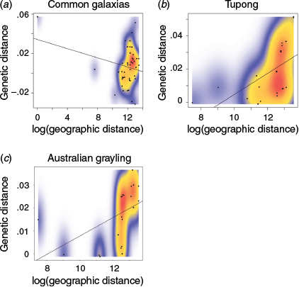
Spatial scales of genetic connectivity, IBD
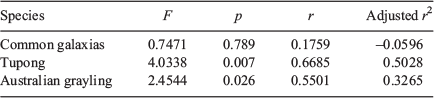
A significant pattern of IBD was observed in tupong (r2 = 0.3279, P = 0.003) and Australian grayling (r2 = 0.2384, P = 0.025) using Mantel tests, whereas no significant pattern was observed in common galaxias (r2 = 0.001375, P = 0.544; Fig. 5). The results obtained through dbRDA were consistent with the results of the Mantel tests, showing no significant relationship for common galaxias (adjusted r2 = –0.0596, P = 0.79) and a clear relationship between pairwise FST and geographic distance in tupong (adjusted r2 = 0.5028, P = 0.007) and Australian grayling (adjusted r2 = 0.3265, P = 0.026; Table 4).
|
|
Evidence of asymmetrical migration between populations
Across every species, asymmetrical migration rates were non-significant between river populations (Tables S16–S20 in the divMigrate results section of the Supplementary material). Tupong and Australian grayling were additionally analysed for migration between the genetically distinct regions found through Structure analysis (structuring found as the western, central, and eastern regions of the Victorian coast). After restructuring by these areas, divMigrate was run for analysis of asymmetrical migration between the regions, but all differing migration rates between each region for both species were non-significant (Tables S19, S20). No spatial population structuring was found for common galaxias using Structure and so no regional migration analysis was undertaken.
Effects of oceanic conditions on population genetic connectivity and migration
For each species, the optimal resistance model to describe population genetic connectivity varied (Table 5). For common galaxias, the optimal resistance model was Model 3, describing larvae that are not affected by current speed or direction and with a preference to water further from the coast. However, this model was non-significant and showed little correlation between raster resistance and pairwise FST (P = 0.3595, r2 = 0.0196). For common galaxias, models using asymmetrical migration rates performed worse than models using pairwise FST, and models not including current information performed slightly better than models including these data, except for Model 1, which performed worse than Model 5 (Table 5). All models developed for common galaxias were non-significant (Table 5).

|
For tupong, the optimal resistance model was Model 1, describing larvae that are not affected by current speed or direction and with no preference to water further or closer to the coastline (Table 5). This model showed a very high and significant correlation between raster resistance and pairwise FST (r2 = 0.5722, P < 0.00007245). For tupong, models using asymmetrical migration rates performed worse than models using pairwise FST, and models not including current information performed slightly better than models using these data, except for Model 3, which performed worse than Models 4–6 (Table 5). All FST-based models for tupong were significant and each yielded a greater correlation than was observed using just Mantel statistics or dbRDA (Tables 4, 5; Fig. 5).
For Australian grayling, the optimal resistance model was Model 2, describing larvae that are not affected by current speed or direction but show a preference for waters closer to the coastline (Table 5). This model showed a very high and significant correlation between raster resistance and pairwise FST (r2 = 0.455, P < 0.0007977). For Australian grayling models using asymmetrical migration, rates performed worse than models using pairwise FST, but models that included current speed and direction performed a mix of better and worse than the non-current models (in order of best model: Models 2, 4, 5, 1, 6, 3). All FST-based models for Australian grayling were significant and all except Models 3 and 6 yielded a greater correlation than was observed just using Mantel statistics or dbRDA (Tables 4,5, Fig. 5).
Effective population sizes
Three distinct genetic regions were identified within tupong and Australian grayling. Using these genetic regions, individuals from each species were pooled into their respective spatial cluster. The values generated for the eastern and western regions were incalculable (returned estimates which generated confidence ranges overlapping with infinity) for all species, likely due to low population sizes (Table 6). Values were generated for each species for the central Victorian region identified (through Structure), and so were used as the primary comparison between the three species. From this region, the effective population size of tupong across both allele frequency tests (full-siblings included: for PCrit = 0.05, Ne = 112.6 (CI 111.5–113.7) and for PCrit = 0.02, Ne = 118.4 (CI 117.3–119.6); siblings removed: for PCrit = 0.05, Ne = 1825.5 (CI 1583.6–2154.1) and for PCrit = 0.02, Ne = 1810.4 (CI 1583.3–2111.3) was significantly lower than for common galaxias (full-siblings included: for PCrit = 0.05, Ne = 692.6 (CI 675.6–710.6) and for PCrit = 0.02, Ne = 670.3 (CI 659.2–681.7); siblings removed: for PCrit = 0.05, Ne = 11 447.8 (CI 8102.1–19 483.7) and for PCrit = 0.02, Ne = 17 362.0 (CI 12 166.9–30 278.3), and varied between slightly higher and lower than Australian grayling (full-siblings included: for PCrit = 0.05, Ne = 1107.6 (CI 1035.4–1190.4) and for PCrit = 0.02, Ne = 1171.5 (CI 1123.7–1223.5); siblings removed: for PCrit = 0.05, Ne = 1124.3 (CI 1136.1–1326.8) and for PCrit = 0.02, Ne = 1295.8 (CI 1237.1–1360.2); Table 6).

|
Discussion
In this study we investigated the genetic connectivity and genetic diversity of three diadromous Australian fish species. Common galaxias exhibited no clear pattern of spatial genetic structuring and high genetic connectivity across the Victorian coastline (~700 km), whereas tupong exhibited moderate population genetic structuring and evidence of an IBD effect. Australian grayling showed some population genetic structuring and evidence of IBD, but to a lesser degree than tupong. In all three species, there was little evidence that oceanic conditions, such as distance from the coast, current strength and current direction, affected genetic connectivity. In addition, there was no evidence of oceanic conditions driving different relative migration rates between populations for any of the species studied. The lack of consistency in connectivity patterns highlights the importance of species-specific studies of population connectivity to inform the management of target species.
Differences in population structuring among species
The results of Structure, FST analysis and DAPC suggested a clear pattern of population structuring for tupong and Australian grayling, and a pattern of high connectivity for common galaxias, across a large spatial scale (~700 km). These patterns are consistent with what is known for tupong and common galaxias from previous genetic studies (Zemlak et al. 2010; Schmidt et al. 2014; Hickford and Schiel 2016). Common galaxias is considered highly dispersive with strong connectivity across the scale of several hundred kilometres in New Zealand and Chile (Zemlak et al. 2010; Hickford and Schiel 2016). Although some population structuring has been observed for different diadromous common galaxias populations, it tends to be at the scale of >1000 km, or driven by glacial events (e.g. along the southern coast of Chile; Zemlak et al. 2010; González-Wevar et al. 2015). Because the scale of the present study was approximately 1000 km for common galaxias, the observation of high connectivity is not unexpected. The pattern of IBD in tupong also supports previous work measuring the genetic connectivity of the species that found a consistent moderate pattern of IBD across the Victorian coast, but provides greater resolution than reported in the previous work, which used microsatellites (Schmidt et al. 2014). Previous genetic analysis of Australian grayling revealed low genetic structuring, but this was undertaken on a smaller spatial scale and used less informative genetic (microsatellite and mitochondrial specifically) markers (Schmidt et al. 2011). Because the present study found evidence of slight population structuring between populations from central and eastern Victoria, the greater resolution of markers used is likely detecting more subtle signatures of population differentiation. The reasons for the differing connectivity between species could be the result of several factors, ranging from environmental conditions present during larval stages through to biological factors such as certain life history traits.
Oceanographic currents provide little insight into the genetic connectivity of species
The Victorian coast is the point at which two strong and opposing currents, namely the EAC and SAC, end (Tilburg et al. 2001; Ridgway and Condie 2004). These currents have been shown to influence the population connectivity of species in different ways, including driving southerly asymmetrical gene flow in the estuary perch (EAC) or easterly gene flow in intertidal molluscs (SAC; Shaddick et al. 2011; Miller et al. 2013). In the present study, tupong and Australian grayling showed population structuring across Victoria. However, both species showed a lack of asymmetrical migration between populations or between regional clusters. This, coupled with resistance models, which showed lower correlation when oceanic conditions were included, suggests that contemporary oceanic conditions are not strongly influencing genetic connectivity within these species. Instead, given the clear pattern of IBD observed in all analyses performed, the pattern of spatial structuring seen within tupong and Australian grayling is likely predominantly the result of IBD.
Although we did not detect any evidence for an effect of ocean currents on patterns of genetic connectivity, our study sites are essentially at the end of the prevailing currents, and it has been demonstrated that the EAC is relatively weaker feeding into Bass Strait than when moving south along the Australian east coast (Ridgway 2007). If individuals were sampled from this wider range, a stronger influence of these currents may have been observed, as can be seen in other studies of species that extend beyond the ranges sampled here (Booth et al. 2007; Shaddick et al. 2011). In addition, although ocean currents may not be driving the patterns of connectivity observed, this does not mean that oceanic conditions play no role. Currents are known to be highly variable, fluctuating on scales as low as metres and varying over the scale of hours (Hays 2017). The lack of effect of oceanic conditions within the studied species may reflect averages failing to represent the true complexity of currents that may be influencing connectivity. Although these fine-scale oceanic patterns can be better incorporated into seascape genetics and connectivity, they require more robust knowledge of target species’ life history traits and the use of simulated dispersal events, which was not achievable with the study species investigated here (Paris et al. 2013).
Potential biological determinants of population structuring
Although many life history traits are poorly understood for the study species, two traits that shape dispersal and overall population connectivity within a species (fecundity and pelagic larval duration, PLD) have been studied for each species (Miles 2007; Clobert et al. 2012). For example, high fecundity has been shown to result in higher connectivity in fish species and marine dispersing organisms in general (Bradbury and Bentzen 2007; Woodings et al. 2018). Fecundity varied by a factor of 10–100 among our study species (Berra 1982; McDowall et al. 1994; Zampatti et al. 2010; Bice et al. 2012; Walker and Humphries 2013). If species connectivity patterns reflect fecundity differences, we would expect higher fecund species to be the most genetically connected. By contrast, fecundity was highest in the least genetically connected species (tupong) and lowest in the most genetically connected species (common galaxias). This suggests that the connectivity differences among species were unlikely to be related to fecundity.
Another key life history trait for diadromous species is PLD, with longer PLD being associated with greater dispersal potential (Selkoe and Toonen 2011). This trait aligns most closely with the observed patterns of connectivity, with common galaxias exhibiting the equal longest PLD along with Australian grayling (4–6 months), and tupong exhibiting the shortest (~120 days; Crook et al. 2006; Jung et al. 2009; Bice et al. 2018). Therefore, PLD, as an absolute number of days, may explain the higher connectivity seen in common galaxias and lower connectivity in tupong but does not explain the population structuring seen in Australian grayling. Further, the lengths of the PLD observed for each species are all considered very long compared with many other highly connected diadromous species (Feutry et al. 2012, 2013; Taillebois et al. 2012; Teichert et al. 2012). When comparing the PLD of each species to reviews across hundreds of studied fish (both diadromous and marine), the PLD of each species studied here suggests that these species should have the capacity to disperse up to thousands of kilometres when not limited by physical geographic factors (Shanks et al. 2003; Selkoe and Toonen 2011; Faurby and Barber 2012). When looking at examples of other small-bodied diadromous species, specifically Kuhlia sauvagii, Kuhlia rupestris (rock flagtail), Sicyopus zosterophorum (belted rockclimbing goby), Smilosicyopus chloe (bilitvat), Akihito vanuatu (Vanuatu’s emperor) and Cotylopus acutipinnis (bichique), they all have PLD between two- and fivefold shorter than any species studied here while maintaining genetic connectivity across ranges of similar or larger size than the coast of Victoria (Feutry et al. 2012, 2013; Taillebois et al. 2012; Teichert et al. 2012). Although PLD is considered a crucial component of effective connectivity for diadromous species, many other life history traits (e.g. larval size, movement strategies and initial larval length) play important roles in influencing population connectivity, making it difficult to reach any conclusions regarding the effects of life history on any connectivity patterns observed in this study.
Effects of effective population sizes on genetic connectivity
Species differences in the extent of population structuring may reflect differences in effective population size. High effective population sizes maintain genetic homogeneity by mitigating the effects of genetic drift at individual sites, increasing the time taken before population-wide genetic differences occur following isolation (Díaz-Jaimes et al. 2010). The effective population sizes calculated for each species varied depending on the test but, after the removal of siblings to mitigate the downward bias of estimates (Peterman et al. 2016), common galaxias consistently showed effective population sizes an order of magnitude higher than the other two species. The effective population sizes align with the observed patterns of connectivity, with common galaxias exhibiting the largest effective population size, followed by Australian grayling and tupong, which exhibited similar values. It is possible that dispersal of common galaxias is restricted across the study area, but that large population sizes buffer the effect of genetic drift and maintain a signature of high genetic connectivity (Lowe and Allendorf 2010). This interpretation is further supported by the very high genetic diversity levels found for common galaxias in both the present study and in previous work on the species (González-Wevar et al. 2015).
The interpretation of effective population size masking population structuring often ignores the close relationship between dispersal and effective population sizes because highly dispersing species typically show higher effective population sizes (e.g. among highly dispersive bird species; Frankham 1997; Arguedas and Parker 2000; Hung et al. 2017). Further, there are many examples of diadromous species exhibiting high effective population sizes while also exhibiting population structuring (Waples et al. 2010; Cushman et al. 2012; Johnstone et al. 2013). Although these studies do not confirm that dispersal and gene flow were unrestricted across our study area for the common galaxias, they do suggest that over large enough time scales (thousands of years), species with high effective population sizes would show structure if they were not connected. As such, there is no direct evidence to suggest that, in this case, high effective population size is masking strong population structuring within common galaxias.
However, it is worth considering that estimating effective population sizes when the exact number of distinct populations or the exact migration rate is not known can lead to biases in the values returned (Ryman et al. 2014). Specifically, in the present study the presence of structuring and limited migration was found for tupong and Australian grayling. The method used to analyse effective population sizes for each species (linkage disequilibrium) is robust provided most genetically distinct populations across the study range have been sampled and migration rates are relatively low (<10%; Waples and England 2011). Although sampling intensity was not sufficient for accurate estimates of effective population sizes within the eastern and western Victorian genetic clusters for all species, reliable estimates for the central Victorian region were determined. Further, sampling within this central region took place over multiple rivers, and clear population structuring was found between this region and the other two genetic regions for tupong and Australian grayling (suggesting the migration rate is likely not high). These factors together suggest that the linkage disequilibrium methods used here are likely to not be so downwardly biased as to affect the overall pattern of effective population size differences, because common galaxias returned estimates up to an order of magnitude larger for the central Victorian region.
Implications for conservation
Common galaxias and tupong are currently listed as species of least concern under the IUCN status (Bice et al. 2019a, 2019b). By contrast, Australian grayling have been listed as vulnerable species under the Environment Protection and Biodiversity Conservation Act 1999 of Australia. The lower effective population size for Australian grayling is consistent with the reduced range and declining population numbers the species has experienced. In addition, the Australian grayling appears to exhibit a moderate degree of IBD across the spatial scale of the Victorian coast, suggesting population connectivity may be limited. Although the pattern of IBD is not as strong compared with tupong, local-scale management of the species to reflect the less-connected nature of distant river populations is an important consideration. Despite the species exhibiting IBD, it is important to consider there was still genetic connectivity between rivers located over 100 km apart. This suggests that rehabilitation of rivers along the Victorian coast may still be an appropriate strategy for the species to recover and repopulate additional river systems, provided source river populations are not great distances away because, over successive generations, individuals can recolonise. Further, as Australian grayling juveniles have been shown to be attracted to downstream water flow from rivers, targeted water flow offers a promising method to direct individuals to specific rivers and promote connectivity or recolonisation into new rivers (Koster et al. 2021).
Although tupong is listed as of least concern, the species was found to have similar effective population sizes to Australian grayling. Tupong also showed a moderate pattern of IBD, suggesting overall connectivity for the species is limited. Of the three species studied, tupong is likely to be the most vulnerable to human-induced disruptions to connectivity (e.g. dams and barriers blocking passage along a river, or to estuaries), with most recruitment occurring at a local scale for this species. Given these findings, as recommended for Australian grayling, conservation of tupong should consider local-scale management of the species, while further work on measuring population sizes should be undertaken as part of regular management practices. Further, because tupong is likely restricted in inter-riverine connectivity, barriers that block downstream migration and spawning in a river may have significant effects on the population size of that river: any reduction in recruitment success will not be offset by migrants from other rivers to the same degree as a more connected species. Because of this, tupong will likely benefit from local river connectivity restoration and may be an ideal indicator species for the effectiveness of such river connectivity restoration projects (e.g. fishways and environmental flows). Such potential benefits can be seen in targeted environmental releases resulting in a movement increase of almost 40% for tupong. Although tupong is currently listed as a species of least concern, active management may be required to prevent future population decline (Department for Environment and Heritage 2003). One promising avenue of active management includes the use of environmental flows to direct migration towards specific rivers, which has shown some effect on several Victorian diadromous species, although exactly how strong this relationship is for tupong is not fully known (Amtstaetter et al. 2021).
When implementing conservation strategies reflective of connectivity, it is important to consider that genetic connectivity is not the same as demographic connectivity. Although many rivers were shown to be genetically connected, comparatively few migrants are needed to move between rivers to maintain genetic connectivity (Lowe and Allendorf 2010). From a practical perspective, this means that localised recruitment can still be the norm, a possibility that is supported by all siblings identified being found within the same river in this study. As such, it is important to not consider genetically connected populations as a single demographic population that allows dispersal across hundreds of kilometres for single individuals; instead, connectivity may take place over multiple generations.
Conclusions
Connectivity is crucial for effective species management, particularly for riverine and diadromous species. This study shows that species with many similar life history traits, and that use a shared environment, can still vary greatly in the extent of genetic connectivity. This work reveals the complex nature of species-level connectivity, emphasising the importance of directly measuring the population connectivity of target species and using that evidence to directly inform management strategies for different species. The use of genomics to measure genetic connectivity offers an effective way to measure connectivity, providing insights into genetic connectivity that can be used to help guide conservation and management across different species and inform how connectivity takes place at a population level. The value of such analyses is particularly clear for species that disperse in marine environments, because the dispersing larvae are often numerous and difficult to track using direct tracking methods.
Data accessibility
The raw genetic data for each species (.csv), and the R code (.R) used to filter each dataset can be found at Open at La Trobe, https://opal.latrobe.edu.au/, under doi: 10.26181/60ac9e770f631.
Conflicts of interest
The authors declare that they have no conflicts of interest.
Declaration of funding
This work was funded by the La Trobe University ABC Research Funding Scheme 2017 – Securing Food Water and the Environment RFA. James O’Dwyer was supported by the Holsworth Wildlife Research Endowment, The Murray–Darling Basin joint governments Centre for Freshwater Ecosystems PhD scholarship and an Australian Postgraduate Award through La Trobe University. Katherine Harrisson was supported by an ARC Discovery Early Career Researcher Award (DECRA) Fellowship (DE190100636).
Acknowledgements
The authors thank Justin O’Connor, Andrew Pickworth, Renae Ayres, Lauren Johnson, Jason Lieschke, Joanne Kearns, Chris Jones and John Mahoney at the Arthur Rylah Institute for sample collection. The authors also thank Nicole Wilson for assistance with genetic diversity analysis, Sarah Willington for sample and database curation and Erin Hill, Simone Currie, Matthew Quin, Jude Hatley, Claire Hutton, Liam Hunt and Jessica Taylor for feedback on the manuscript. The authors thank two anonymous reviewers for the feedback provided on the manuscript.
References
Allen, G. R., Midgley, S. H., and Allen, M. (2002) ‘Field Guide to the Freshwater Fishes of Australia.’ (Western Australian Museum: Perth, WA, Australia.)Almany, G. R., Connolly, S. R., Heath, D. D., Hogan, J. D., Jones, G. P., McCook, L. J., Mills, M., Pressey, R. L., and Williamson, D. H. (2009). Connectivity, biodiversity conservation and the design of marine reserve networks for coral reefs. Coral Reefs 28, 339–351.
| Connectivity, biodiversity conservation and the design of marine reserve networks for coral reefs.Crossref | GoogleScholarGoogle Scholar |
Amtstaetter, F., Tonkin, Z., O’Connor, J., Stuart, I., and Koster, W. M. (2021). Environmental flows stimulate the upstream movement of juvenile diadromous fishes. Marine and Freshwater Research 72, 1019–1026.
| Environmental flows stimulate the upstream movement of juvenile diadromous fishes.Crossref | GoogleScholarGoogle Scholar |
Arguedas, N., and Parker, P. G. (2000). Seasonal migration and genetic population structure in house wrens. The Condor 102, 517–528.
| Seasonal migration and genetic population structure in house wrens.Crossref | GoogleScholarGoogle Scholar |
Baird, M. E., Timko, P. G., Suthers, I. M., and Middleton, J. H. (2006). Coupled physical–biological modelling study of the East Australian Current with idealised wind forcing. Part I: biological model intercomparison. Journal of Marine Systems 59, 249–270.
| Coupled physical–biological modelling study of the East Australian Current with idealised wind forcing. Part I: biological model intercomparison.Crossref | GoogleScholarGoogle Scholar |
Berra, T. M. (1982). Life history of the Australian grayling, Prototroctes maraena (Salmoniformes: Prototroctidae) in the Tambo River, Victoria. Copeia 1982, 795–805.
| Life history of the Australian grayling, Prototroctes maraena (Salmoniformes: Prototroctidae) in the Tambo River, Victoria.Crossref | GoogleScholarGoogle Scholar |
Bice, C., Zampatti, B., Jennings, P., and Wilson, P. (2012) Fish assemblage structure, movement and recruitment in the Coorong and Lower Lakes in 2011/12. SARDI Publication number F2011/000186-3. (SARDI Aquatic Sciences: Adelaide, SA, Australia.) Available at https://www.pir.sa.gov.au/__data/assets/pdf_file/0015/232215/Coorong_Fish_Movement_11_12_Report.pdf
Bice, C. M., Zampatti, B. P., and Morrongiello, J. R. (2018). Connectivity, migration and recruitment in a catadromous fish. Marine and Freshwater Research 69, 1733–1745.
| Connectivity, migration and recruitment in a catadromous fish.Crossref | GoogleScholarGoogle Scholar |
Bice, C., Gilligan, D., and Koehn, J. (2019a) Congolli Pseudaphritis urvillii. In ‘The IUCN Red List of Threatened Species 2019’. e.T122913501A123382361. (International Union for Conservation of Nature and Natural Resources.) Available at https://www.iucnredlist.org/species/122913501/123382361 [Verified 18 May 2021].
Bice, C., Raadik, T., David, B., West, D., Franklin, P., Allibone, R., Ling, N., Hitchmough, R., and Crow, S. (2019b) Common galaxias Galaxias maculatus. In ‘The IUCN Red List of Threatened Species 2019’. e.T197279A129040788. (International Union for Conservation of Nature and Natural Resources.) Available at https://www.iucnredlist.org/species/197279/129040788 [Verified 18 May 2021].
Birnie-Gauvin, K., Tummers, J. S., Lucas, M. C., and Aarestrup, K. (2017). Adaptive management in the context of barriers in European freshwater ecosystems. Journal of Environmental Management 204, 436–441.
| Adaptive management in the context of barriers in European freshwater ecosystems.Crossref | GoogleScholarGoogle Scholar | 28917178PubMed |
Bitume, E. V., Bonte, D., Ronce, O., Bach, F., Flaven, E., Olivieri, I., and Nieberding, C. M. (2013). Density and genetic relatedness increase dispersal distance in a subsocial organism. Ecology Letters 16, 430–437.
| Density and genetic relatedness increase dispersal distance in a subsocial organism.Crossref | GoogleScholarGoogle Scholar | 23294510PubMed |
Bitume, E. V., Bonte, D., Ronce, O., Olivieri, I., and Nieberding, C. M. (2014). Dispersal distance is influenced by parental and grand-parental density. Proceedings of the Royal Society of London – B. Biological Sciences 281, 20141061.
| Dispersal distance is influenced by parental and grand-parental density.Crossref | GoogleScholarGoogle Scholar |
Bonte, D., and Dahirel, M. (2017). Dispersal: a central and independent trait in life history. Oikos 126, 472–479.
| Dispersal: a central and independent trait in life history.Crossref | GoogleScholarGoogle Scholar |
Booth, D. J., Figueira, W. F., Gregson, M. A., Brown, L., and Beretta, G. (2007). Occurrence of tropical fishes in temperate southeastern Australia: role of the East Australian Current. Estuarine, Coastal and Shelf Science 72, 102–114.
| Occurrence of tropical fishes in temperate southeastern Australia: role of the East Australian Current.Crossref | GoogleScholarGoogle Scholar |
Bradbury, I. R., and Bentzen, P. (2007). Non-linear genetic isolation by distance. Implications for dispersal estimation in anadromous and marine fish populations. Marine Ecology Progress Series 340, 245–257.
| Non-linear genetic isolation by distance. Implications for dispersal estimation in anadromous and marine fish populations.Crossref | GoogleScholarGoogle Scholar |
Bradbury, I. R., Laurel, B., Snelgrove, P. V., Bentzen, P., and Campana, S. E. (2008). Global patterns in marine dispersal estimates: the influence of geography, taxonomic category and life history. Proceedings of the Royal Society of London – B. Biological Sciences 275, 1803–1809.
| Global patterns in marine dispersal estimates: the influence of geography, taxonomic category and life history.Crossref | GoogleScholarGoogle Scholar |
Carroll, C., Rohlf, D. J., Li, Y. W., Hartl, B., Phillips, M. K., and Noss, R. F. (2015). Connectivity conservation and endangered species recovery: a study in the challenges of defining conservation‐reliant species. Conservation Letters 8, 132–138.
| Connectivity conservation and endangered species recovery: a study in the challenges of defining conservation‐reliant species.Crossref | GoogleScholarGoogle Scholar |
Clobert, J., Baguette, M., Benton, T. G., and Bullock, J. M. (2012) ‘Dispersal Ecology and Evolution.’ (Oxford University Press: Oxford, UK.)
Cook, C. N., and Sgro, C. M. (2017). Aligning science and policy to achieve evolutionarily enlightened conservation. Conservation Biology 31, 501–512.
| Aligning science and policy to achieve evolutionarily enlightened conservation.Crossref | GoogleScholarGoogle Scholar | 27862324PubMed |
Criscuolo, N. G., and Angelini, C. (2020). StructuRly: a novel shiny app to produce comprehensive, detailed and interactive plots for population genetic analysis. PLoS One 15, e0229330.
| StructuRly: a novel shiny app to produce comprehensive, detailed and interactive plots for population genetic analysis.Crossref | GoogleScholarGoogle Scholar | 32074134PubMed |
Crook, D. A., Macdonald, J. I., O’Connor, J. P., and Barry, B. (2006). Use of otolith chemistry to examine patterns of diadromy in the threatened Australian grayling Prototroctes maraena. Journal of Fish Biology 69, 1330–1344.
| Use of otolith chemistry to examine patterns of diadromy in the threatened Australian grayling Prototroctes maraena.Crossref | GoogleScholarGoogle Scholar |
Crook, D. A., Koster, W. M., Macdonald, J. I., Nicol, S. J., Belcher, C. A., Dawson, D. R., O’Mahony, D. J., Lovett, D., Walker, A., and Bannam, L. (2010). Catadromous migrations by female tupong (Pseudaphritis urvillii) in coastal streams in Victoria, Australia. Marine and Freshwater Research 61, 474–483.
| Catadromous migrations by female tupong (Pseudaphritis urvillii) in coastal streams in Victoria, Australia.Crossref | GoogleScholarGoogle Scholar |
Cushman, E., Tarpey, C., Post, B., Ware, K., and Darden, T. (2012). Genetic characterization of American shad in the Edisto River, South Carolina, and initial evaluation of an experimental stocking program. Transactions of the American Fisheries Society 141, 1338–1348.
| Genetic characterization of American shad in the Edisto River, South Carolina, and initial evaluation of an experimental stocking program.Crossref | GoogleScholarGoogle Scholar |
Delgado, M. L., and Ruzzante, D. (2020). Investigating diadromy in fishes and its loss in an -omics era. iScience 23, 101837.
| Investigating diadromy in fishes and its loss in an -omics era.Crossref | GoogleScholarGoogle Scholar | 33305191PubMed |
Delgado, M. L., Górski, K., Habit, E., and Ruzzante, D. E. (2019). The effects of diadromy and its loss on genomic divergence: the case of amphidromous Galaxias maculatus populations. Molecular Ecology 28, 5217–5231.
| The effects of diadromy and its loss on genomic divergence: the case of amphidromous Galaxias maculatus populations.Crossref | GoogleScholarGoogle Scholar | 31652382PubMed |
Department for Environment and Heritage (2003) Review of the status of threatened species in South Australia. Proposed Schedules under the South Australian National Parks and Wildlife Act 1972 Discussion Paper. (NPaWC Department for Environment and Heritage).
Díaz-Jaimes, P., Uribe-Alcocer, M., Rocha-Olivares, A., Garcia-de-Leon, F. J., Nortmoon, P., and Durand, J. D. (2010). Global phylogeography of the dolphinfish (Coryphaena hippurus): the influence of large effective population size and recent dispersal on the divergence of a marine pelagic cosmopolitan species. Molecular Phylogenetics and Evolution 57, 1209–1218.
| Global phylogeography of the dolphinfish (Coryphaena hippurus): the influence of large effective population size and recent dispersal on the divergence of a marine pelagic cosmopolitan species.Crossref | GoogleScholarGoogle Scholar | 20971198PubMed |
Do, C., Waples, R. S., Peel, D., Macbeth, G. M., Tillett, B. J., and Ovenden, J. R. (2014). NeEstimator v2: re-implementation of software for the estimation of contemporary effective population size (Ne) from genetic data. Molecular Ecology Resources 14, 209–214.
| NeEstimator v2: re-implementation of software for the estimation of contemporary effective population size (Ne) from genetic data.Crossref | GoogleScholarGoogle Scholar | 23992227PubMed |
Earl, D. A. (2012). STRUCTURE HARVESTER: a website and program for visualizing STRUCTURE output and implementing the Evanno method. Conservation Genetics Resources 4, 359–361.
| STRUCTURE HARVESTER: a website and program for visualizing STRUCTURE output and implementing the Evanno method.Crossref | GoogleScholarGoogle Scholar |
Evanno, G., Regnaut, S., and Goudet, J. (2005). Detecting the number of clusters of individuals using the software STRUCTURE: a simulation study. Molecular Ecology 14, 2611–2620.
| Detecting the number of clusters of individuals using the software STRUCTURE: a simulation study.Crossref | GoogleScholarGoogle Scholar | 15969739PubMed |
Faurby, S., and Barber, P. H. (2012). Theoretical limits to the correlation between pelagic larval duration and population genetic structure. Molecular Ecology 21, 3419–3432.
| Theoretical limits to the correlation between pelagic larval duration and population genetic structure.Crossref | GoogleScholarGoogle Scholar | 22574811PubMed |
Feutry, P., Valade, P., Ovenden, J. R., Lopez, P. J., and Keith, P. (2012). Pelagic larval duration of two diadromous species of Kuhliidae (Teleostei: Percoidei) from Indo-Pacific insular systems. Marine and Freshwater Research 63, 397–402.
| Pelagic larval duration of two diadromous species of Kuhliidae (Teleostei: Percoidei) from Indo-Pacific insular systems.Crossref | GoogleScholarGoogle Scholar |
Feutry, P., Vergnes, A., Broderick, D., Lambourdière, J., Keith, P., and Ovenden, J. R. (2013). Stretched to the limit; can a short pelagic larval duration connect adult populations of an Indo-Pacific diadromous fish (Kuhlia rupestris)? Molecular Ecology 22, 1518–1530.
| Stretched to the limit; can a short pelagic larval duration connect adult populations of an Indo-Pacific diadromous fish (Kuhlia rupestris)?Crossref | GoogleScholarGoogle Scholar | 23294379PubMed |
Foll, M., and Gaggiotti, O. (2008). A genome-scan method to identify selected loci appropriate for both dominant and codominant markers: a Bayesian perspective. Genetics 180, 977–993.
| A genome-scan method to identify selected loci appropriate for both dominant and codominant markers: a Bayesian perspective.Crossref | GoogleScholarGoogle Scholar | 18780740PubMed |
Frankham, R. (1997). Do island populations have less genetic variation than mainland populations? Heredity 78, 311–327.
| Do island populations have less genetic variation than mainland populations?Crossref | GoogleScholarGoogle Scholar | 9119706PubMed |
Frankham, R. (2005). Genetics and extinction. Biological Conservation 126, 131–140.
| Genetics and extinction.Crossref | GoogleScholarGoogle Scholar |
Frankham, R. (2007). Effective population size/adult population size ratios in wildlife: a review. Genetical Research 89, 491–503.
| Effective population size/adult population size ratios in wildlife: a review.Crossref | GoogleScholarGoogle Scholar | 18976539PubMed |
Friesen, V. L. (2015). Speciation in seabirds: why are there so many species … and why aren’t there more? Journal of Ornithology 156, 27–39.
| Speciation in seabirds: why are there so many species … and why aren’t there more?Crossref | GoogleScholarGoogle Scholar |
Fumagalli, M. (2013). Assessing the effect of sequencing depth and sample size in population genetics inferences. PLoS One 8, e79667.
| Assessing the effect of sequencing depth and sample size in population genetics inferences.Crossref | GoogleScholarGoogle Scholar | 24260275PubMed |
Gomon, M. F., and Bray, D. J. (2011) Common galaxias, Galaxias maculatus (Jenyns 1842). In ‘Fishes of Australia’. (Museums Victoria on behalf of the OzFishNet community.) Available at https://fishesofaustralia.net.au/home/species/2129
Gomon, M. F., Bray, D. J., and Kuiter, R. H. (2008) ‘Fishes of Australia’s Southern Coast.’ (Reed New Holland.)
González-Wevar, C. A., Salinas, P., Hüne, M., Segovia, N. I., Vargas-Chacoff, L., Astorga, M., Cañete, J. I., and Poulin, E. (2015). Phylogeography in Galaxias maculatus (Jenyns, 1848) along two biogeographical provinces in the Chilean coast. PLoS One 10, e0131289.
| Phylogeography in Galaxias maculatus (Jenyns, 1848) along two biogeographical provinces in the Chilean coast.Crossref | GoogleScholarGoogle Scholar | 26161896PubMed |
Goudet, J. (2005). Hierfstat, a package for R to compute and test hierarchical F‐statistics. Molecular Ecology Notes 5, 184–186.
| Hierfstat, a package for R to compute and test hierarchical F‐statistics.Crossref | GoogleScholarGoogle Scholar |
Gruber, B., Unmack, P. J., Berry, O. F., and Georges, A. (2018). dartr: An r package to facilitate analysis of SNP data generated from reduced representation genome sequencing. Molecular Ecology Resources 18, 691–699.
| dartr: An r package to facilitate analysis of SNP data generated from reduced representation genome sequencing.Crossref | GoogleScholarGoogle Scholar | 29266847PubMed |
Haddad, N. M., Brudvig, L. A., Clobert, J., Davies, K. F., Gonzalez, A., Holt, R. D., Lovejoy, T. E., Sexton, J. O., Austin, M. P., Collins, C. D., Cook, W. M., Damschen, E. I., Ewers, R. M., Foster, B. L., Jenkins, C. N., King, A. J., Laurance, W. F., Levey, D. J., Margules, C. R., Melbourne, B. A., Nicholls, A. O., Orrock, J. L., Song, D. X., and Townshend, J. R. (2015). Habitat fragmentation and its lasting impact on Earth’s ecosystems. Science Advances 1, e1500052.
| Habitat fragmentation and its lasting impact on Earth’s ecosystems.Crossref | GoogleScholarGoogle Scholar | 26601154PubMed |
Hanski, I. (1998). Metapopulation dynamics. Nature 396, 41–49.
| Metapopulation dynamics.Crossref | GoogleScholarGoogle Scholar |
Hays, G. C. (2017). Ocean currents and marine life. Current Biology 27, R470–R473.
| Ocean currents and marine life.Crossref | GoogleScholarGoogle Scholar | 28586681PubMed |
Hickford, M. J., and Schiel, D. R. (2016). Otolith microchemistry of the amphidromous Galaxias maculatus shows recruitment to coastal rivers from unstructured larval pools. Marine Ecology Progress Series 548, 197–207.
| Otolith microchemistry of the amphidromous Galaxias maculatus shows recruitment to coastal rivers from unstructured larval pools.Crossref | GoogleScholarGoogle Scholar |
Hung, C. M., Drovetski, S. V., and Zink, R. M. (2017). The roles of ecology, behaviour and effective population size in the evolution of a community. Molecular Ecology 26, 3775–3784.
| The roles of ecology, behaviour and effective population size in the evolution of a community.Crossref | GoogleScholarGoogle Scholar | 28437589PubMed |
Jakobsson, M., and Rosenberg, N. A. (2007). CLUMPP: a cluster matching and permutation program for dealing with label switching and multimodality in analysis of population structure. Bioinformatics 23, 1801–1806.
| CLUMPP: a cluster matching and permutation program for dealing with label switching and multimodality in analysis of population structure.Crossref | GoogleScholarGoogle Scholar | 17485429PubMed |
Jansson, R., Nilsson, C., and Malmqvist, B. (2007). Restoring freshwater ecosystems in riverine landscapes: the roles of connectivity and recovery processes. Freshwater Biology 52, 589–596.
| Restoring freshwater ecosystems in riverine landscapes: the roles of connectivity and recovery processes.Crossref | GoogleScholarGoogle Scholar |
Johnstone, D. L., O’Connell, M. F., Palstra, F. P., and Ruzzante, D. E. (2013). Mature male parr contribution to the effective size of an anadromous Atlantic salmon (Salmo salar) population over 30 years. Molecular Ecology 22, 2394–2407.
| Mature male parr contribution to the effective size of an anadromous Atlantic salmon (Salmo salar) population over 30 years.Crossref | GoogleScholarGoogle Scholar | 23317429PubMed |
Jones, P. E., and Closs, G. P. (2016). Interspecific differences in larval production and dispersal in non-migratory galaxiids: implications for metapopulation structure. Marine and Freshwater Research 67, 1479–1492.
| Interspecific differences in larval production and dispersal in non-migratory galaxiids: implications for metapopulation structure.Crossref | GoogleScholarGoogle Scholar |
Jones, O. R., and Wang, J. (2010). COLONY: a program for parentage and sibship inference from multilocus genotype data. Molecular Ecology Resources 10, 551–555.
| COLONY: a program for parentage and sibship inference from multilocus genotype data.Crossref | GoogleScholarGoogle Scholar | 21565056PubMed |
Jung, C. A., Barbee, N. C., and Swearer, S. E. (2009). Post-settlement migratory behaviour and growth-related costs in two diadromous fish species, Galaxias maculatus and Galaxias brevipinnis. Journal of Fish Biology 75, 503–515.
| Post-settlement migratory behaviour and growth-related costs in two diadromous fish species, Galaxias maculatus and Galaxias brevipinnis.Crossref | GoogleScholarGoogle Scholar | 20738553PubMed |
Kilian, A., Wenzl, P., Huttner, E., Carling, J., Xia, L., Blois, H., Caig, V., Heller-Uszynska, K., Jaccoud, D., Hopper, C., Aschenbrenner-Kilian, M., Evers, M., Peng, K., Cayla, C., Hok, P., and Uszynski, G. (2012) Diversity arrays technology: a generic genome profiling technology on open platforms. In ‘Data Production and Analysis in Population Genomics: Methods and Protocols’. (Eds F Pompanon and A Bonin.) pp. 67–89. (Humana Press: Totowa, NJ, USA)
Koster, W., and Gilligan, D. (2019) Australian grayling Prototroctes maraena. In ‘The IUCN Red List of Threatened Species 2019’. e.T18383A123378802. (International Union for Conservation of Nature and Natural Resources.) Available at https://www.iucnredlist.org/species/18383/123378802 [Verified 18 May 2021].
Koster, W. M., Dawson, D. R., and Crook, D. A. (2013). Downstream spawning migration by the amphidromous Australian grayling (Prototroctes maraena) in a coastal river in south-eastern Australia. Marine and Freshwater Research 64, 31–41.
| Downstream spawning migration by the amphidromous Australian grayling (Prototroctes maraena) in a coastal river in south-eastern Australia.Crossref | GoogleScholarGoogle Scholar |
Koster, W. M., Crook, D. A., Dawson, D. R., Gaskill, S., and Morrongiello, J. R. (2018). Predicting the influence of streamflow on migration and spawning of a threatened diadromous fish, the Australian grayling Prototroctes maraena. Environmental Management 61, 443–453.
| Predicting the influence of streamflow on migration and spawning of a threatened diadromous fish, the Australian grayling Prototroctes maraena.Crossref | GoogleScholarGoogle Scholar | 28374227PubMed |
Koster, W. M., Amtstaetter, F., Dawson, D., Coleman, R. A., and Hale, R. (2021). Environmental influences on the juvenile migration of the threatened amphidromous Australian grayling (Prototroctes maraena). Marine and Freshwater Research 72, 411–417.
| Environmental influences on the juvenile migration of the threatened amphidromous Australian grayling (Prototroctes maraena).Crossref | GoogleScholarGoogle Scholar |
Lowe, W. H., and Allendorf, F. W. (2010). What can genetics tell us about population connectivity? Molecular Ecology 19, 3038–3051.
| What can genetics tell us about population connectivity?Crossref | GoogleScholarGoogle Scholar | 20618697PubMed |
Magris, R. A., Treml, E. A., Pressey, R. L., and Weeks, R. (2016). Integrating multiple species connectivity and habitat quality into conservation planning for coral reefs. Ecography 39, 649–664.
| Integrating multiple species connectivity and habitat quality into conservation planning for coral reefs.Crossref | GoogleScholarGoogle Scholar |
McDowall, R. M. (1988) ‘Diadromy in Fishes: Migrations between Freshwater and Marine Environments.’ (Timber Press, Incorporated.)
McDowall, R. (1999). Different kinds of diadromy: different kinds of conservation problems. ICES Journal of Marine Science 56, 410–413.
| Different kinds of diadromy: different kinds of conservation problems.Crossref | GoogleScholarGoogle Scholar |
McDowall, R. M. (2000) ‘The Reed Field Guide to New Zealand Freshwater Fishes.’ (Reed Publishing, Auckland, New Zealand.)
McDowall, R., Mitchell, C., and Brothers, E. (1994). Age at migration from the sea of juvenile galaxias in New Zealand (Pisces: Galaxiidae). Bulletin of Marine Science 54, 385–402.
Miles, N. (2007) Biology and Ecology of Diadromous Fishes in South Eastern Australia. Ph.D. Thesis, The University of Wollongong, Wollongong, NSW, Australia
Miller, A. D., Versace, V. L., Matthews, T. G., Montgomery, S., and Bowie, K. C. (2013). Ocean currents influence the genetic structure of an intertidal mollusc in southeastern Australia – implications for predicting the movement of passive dispersers across a marine biogeographic barrier. Ecology and Evolution 3, 1248–1261.
| Ocean currents influence the genetic structure of an intertidal mollusc in southeastern Australia – implications for predicting the movement of passive dispersers across a marine biogeographic barrier.Crossref | GoogleScholarGoogle Scholar | 23762511PubMed |
Myers, G. S. (1949). Usage of anadromous, catadromous and allied terms for migratory fishes. Copeia 1949, 89–97.
| Usage of anadromous, catadromous and allied terms for migratory fishes.Crossref | GoogleScholarGoogle Scholar |
Noss, R. F., Dobson, A. P., Baldwin, R., Beier, P., Davis, C. R., Dellasala, D. A., Francis, J., Locke, H., Nowak, K., Lopez, R., Reining, C., Trombulak, S. C., and Tabor, G. (2012). Bolder thinking for conservation. Conservation Biology 26, 1–4.
| Bolder thinking for conservation.Crossref | GoogleScholarGoogle Scholar | 22280321PubMed |
Paris, C. B., Helgers, J., van Sebille, E., and Srinivasan, A. (2013). Connectivity Modeling System: a probabilistic modeling tool for the multi-scale tracking of biotic and abiotic variability in the ocean. Environmental Modelling & Software 42, 47–54.
| Connectivity Modeling System: a probabilistic modeling tool for the multi-scale tracking of biotic and abiotic variability in the ocean.Crossref | GoogleScholarGoogle Scholar |
Pascual, M., Rives, B., Schunter, C., and Macpherson, E. (2017). Impact of life history traits on gene flow: a multispecies systematic review across oceanographic barriers in the Mediterranean Sea. PLoS One 12, e0176419.
| Impact of life history traits on gene flow: a multispecies systematic review across oceanographic barriers in the Mediterranean Sea.Crossref | GoogleScholarGoogle Scholar | 28489878PubMed |
Pebesma, E. J. (2018). Simple features for R: standardized support for spatial vector data. The R Journal 10, 439–446.
| Simple features for R: standardized support for spatial vector data.Crossref | GoogleScholarGoogle Scholar |
Peterman, W., Brocato, E. R., Semlitsch, R. D., and Eggert, L. S. (2016). Reducing bias in population and landscape genetic inferences: the effects of sampling related individuals and multiple life stages. PeerJ 4, e1813.
| Reducing bias in population and landscape genetic inferences: the effects of sampling related individuals and multiple life stages.Crossref | GoogleScholarGoogle Scholar | 26989639PubMed |
Pritchard, J. K., Stephens, M., and Donnelly, P. (2000). Inference of population structure using multilocus genotype data. Genetics 155, 945–959.
| Inference of population structure using multilocus genotype data.Crossref | GoogleScholarGoogle Scholar | 10835412PubMed |
Puebla, O. (2009). Ecological speciation in marine v. freshwater fishes. Journal of Fish Biology 75, 960–996.
| Ecological speciation in marine v. freshwater fishes.Crossref | GoogleScholarGoogle Scholar | 20738594PubMed |
Ridgway, K. R. (2007). Seasonal circulation around Tasmania: an interface between eastern and western boundary dynamics. Journal of Geophysical Research 112, C10016.
| Seasonal circulation around Tasmania: an interface between eastern and western boundary dynamics.Crossref | GoogleScholarGoogle Scholar |
Ridgway, K. R., and Condie, S. A. (2004). The 5500-km-long boundary flow off western and southern Australia. Journal of Geophysical Research 109, C04017.
| The 5500-km-long boundary flow off western and southern Australia.Crossref | GoogleScholarGoogle Scholar |
Riginos, C., Douglas, K. E., Jin, Y., Shanahan, D. F., and Treml, E. A. (2011). Effects of geography and life history traits on genetic differentiation in benthic marine fishes. Ecography 34, 566–575.
| Effects of geography and life history traits on genetic differentiation in benthic marine fishes.Crossref | GoogleScholarGoogle Scholar |
Ryman, N., Allendorf, F. W., Jorde, P. E., Laikre, L., and Hössjer, O. (2014). Samples from subdivided populations yield biased estimates of effective size that overestimate the rate of loss of genetic variation. Molecular Ecology Resources 14, 87–99.
| Samples from subdivided populations yield biased estimates of effective size that overestimate the rate of loss of genetic variation.Crossref | GoogleScholarGoogle Scholar | 24034449PubMed |
Sánchez-Montes, G., Wang, J., Ariño, A. H., and Martínez-Solano, Í. (2018). Mountains as barriers to gene flow in amphibians: quantifying the differential effect of a major mountain ridge on the genetic structure of four sympatric species with different life history traits. Journal of Biogeography 45, 318–331.
| Mountains as barriers to gene flow in amphibians: quantifying the differential effect of a major mountain ridge on the genetic structure of four sympatric species with different life history traits.Crossref | GoogleScholarGoogle Scholar |
Schmidt, D. J., Crook, D. A., O’Connor, J. P., and Hughes, J. M. (2011). Genetic analysis of threatened Australian grayling Prototroctes maraena suggests recruitment to coastal rivers from an unstructured marine larval source population. Journal of Fish Biology 78, 98–111.
| Genetic analysis of threatened Australian grayling Prototroctes maraena suggests recruitment to coastal rivers from an unstructured marine larval source population.Crossref | GoogleScholarGoogle Scholar | 21235548PubMed |
Schmidt, D. J., Crook, D. A., Macdonald, J. I., Huey, J. A., Zampatti, B. P., Chilcott, S., Raadik, T. A., and Hughes, J. M. (2014). Migration history and stock structure of two putatively diadromous teleost fishes, as determined by genetic and otolith chemistry analyses. Freshwater Science 33, 193–206.
| Migration history and stock structure of two putatively diadromous teleost fishes, as determined by genetic and otolith chemistry analyses.Crossref | GoogleScholarGoogle Scholar |
Selkoe, K. A., and Toonen, R. J. (2011). Marine connectivity: a new look at pelagic larval duration and genetic metrics of dispersal. Marine Ecology Progress Series 436, 291–305.
| Marine connectivity: a new look at pelagic larval duration and genetic metrics of dispersal.Crossref | GoogleScholarGoogle Scholar |
Shaddick, K., Moran, P., Gilligan, D. M., Burridge, C. P., Jerry, D. R., Truong, K., and Beheregaray, L. B. (2011). Historic divergence with contemporary connectivity in a catadromous fish, the estuary perch (Macquaria colonorum). Canadian Journal of Fisheries and Aquatic Sciences 68, 304–318.
| Historic divergence with contemporary connectivity in a catadromous fish, the estuary perch (Macquaria colonorum).Crossref | GoogleScholarGoogle Scholar |
Shanks, A. L., Grantham, B. A., and Carr, M. H. (2003). Propagule dispersal distance and the size and spacing of marine reserves. Ecological Applications 13, 159–169.
| Propagule dispersal distance and the size and spacing of marine reserves.Crossref | GoogleScholarGoogle Scholar |
Smith, T. B., Kinnison, M. T., Strauss, S. Y., Fuller, T. L., and Carroll, S. P. (2014). Prescriptive evolution to conserve and manage biodiversity. Annual Review of Ecology, Evolution, and Systematics 45, 1–22.
| Prescriptive evolution to conserve and manage biodiversity.Crossref | GoogleScholarGoogle Scholar |
Stevens, V. M., Trochet, A., Van Dyck, H., Clobert, J., and Baguette, M. (2012). How is dispersal integrated in life histories: a quantitative analysis using butterflies. Ecology Letters 15, 74–86.
| How is dispersal integrated in life histories: a quantitative analysis using butterflies.Crossref | GoogleScholarGoogle Scholar | 22070676PubMed |
Stevens, V. M., Whitmee, S., Le Galliard, J.-F., Clobert, J., Böhning-Gaese, K., Bonte, D., Brändle, M., Matthias Dehling, D., Hof, C., Trochet, A., Baguette, M., and Chase, J. (2014). A comparative analysis of dispersal syndromes in terrestrial and semi-terrestrial animals. Ecology Letters 17, 1039–1052.
| A comparative analysis of dispersal syndromes in terrestrial and semi-terrestrial animals.Crossref | GoogleScholarGoogle Scholar | 24915998PubMed |
Sundqvist, L., Keenan, K., Zackrisson, M., Prodohl, P., and Kleinhans, D. (2016). Directional genetic differentiation and relative migration. Ecology and Evolution 6, 3461–3475.
| Directional genetic differentiation and relative migration.Crossref | GoogleScholarGoogle Scholar | 27127613PubMed |
Taillebois, L., Maeda, K., Vigne, S., and Keith, P. (2012). Pelagic larval duration of three amphidromous Sicydiinae gobies (Teleostei: Gobioidei) including widespread and endemic species. Ecology Freshwater Fish 21, 552–559.
| Pelagic larval duration of three amphidromous Sicydiinae gobies (Teleostei: Gobioidei) including widespread and endemic species.Crossref | GoogleScholarGoogle Scholar |
Teichert, N., Richarson, M., Valade, P., and Gaudin, P. (2012). Reproduction and marine life history of an endemic amphidromous gobiid fish of Reunion Island. Aquatic Biology 15, 225–236.
| Reproduction and marine life history of an endemic amphidromous gobiid fish of Reunion Island.Crossref | GoogleScholarGoogle Scholar |
Thacker, C. E. (2017). Patterns of divergence in fish species separated by the Isthmus of Panama. BMC Evolutionary Biology 17, 111.
| Patterns of divergence in fish species separated by the Isthmus of Panama.Crossref | GoogleScholarGoogle Scholar | 28486928PubMed |
Tilburg, C. E., Hurlburt, H. E., O’Brien, J. J., and Shriver, J. F. (2001). The dynamics of the East Australian Current System: the Tasman Front, the East Auckland Current, and the East Cape Current. Journal of Physical Oceanography 31, 2917–2943.
| The dynamics of the East Australian Current System: the Tasman Front, the East Auckland Current, and the East Cape Current.Crossref | GoogleScholarGoogle Scholar |
van Etten, J. (2017). R Package gdistance: distances and routes on geographical grids. Journal of Statistical Software 76, 1–21.
| R Package gdistance: distances and routes on geographical grids.Crossref | GoogleScholarGoogle Scholar |
Walker, K. F., and Humphries, P. (2013) ‘Ecology of Australian Freshwater Fishes.’ (CSIRO Publishing: Melbourne, Vic., Australia.)
Waples, R. S., and England, P. R. (2011). Estimating contemporary effective population size on the basis of linkage disequilibrium in the face of migration. Genetics 189, 633–644.
| Estimating contemporary effective population size on the basis of linkage disequilibrium in the face of migration.Crossref | GoogleScholarGoogle Scholar | 21840864PubMed |
Waples, R. S., Jensen, D. W., and McClure, M. (2010). Eco-evolutionary dynamics: fluctuations in population growth rate reduce effective population size in chinook salmon. Ecology 91, 902–914.
| Eco-evolutionary dynamics: fluctuations in population growth rate reduce effective population size in chinook salmon.Crossref | GoogleScholarGoogle Scholar | 20426347PubMed |
Ward, R. D., Woodwark, M., and Skibinski, D. O. F. (1994). A comparison of genetic diversity levels in marine, freshwater, and anadromous fishes. Journal of Fish Biology 44, 213–232.
| A comparison of genetic diversity levels in marine, freshwater, and anadromous fishes.Crossref | GoogleScholarGoogle Scholar |
Waters, J. M., Fraser, C. I., and Hewitt, G. M. (2013). Founder takes all: density-dependent processes structure biodiversity. Trends in Ecology & Evolution 28, 78–85.
| Founder takes all: density-dependent processes structure biodiversity.Crossref | GoogleScholarGoogle Scholar |
Whitmee, S., and Orme, C. D. (2013). Predicting dispersal distance in mammals: a trait-based approach. Journal of Animal Ecology 82, 211–221.
| Predicting dispersal distance in mammals: a trait-based approach.Crossref | GoogleScholarGoogle Scholar |
Wilson, M. C., Chen, X.-Y., Corlett, R. T., Didham, R. K., Ding, P., Holt, R. D., Holyoak, M., Hu, G., Hughes, A. C., Jiang, L., Laurance, W. F., Liu, J., Pimm, S. L., Robinson, S. K., Russo, S. E., Si, X., Wilcove, D. S., Wu, J., and Yu, M. (2016). Habitat fragmentation and biodiversity conservation: key findings and future challenges. Landscape Ecology 31, 219–227.
| Habitat fragmentation and biodiversity conservation: key findings and future challenges.Crossref | GoogleScholarGoogle Scholar |
Winter, D. J. (2012). mmod: an R library for the calculation of population differentiation statistics. Molecular Ecology Resources 12, 1158–1160.
| mmod: an R library for the calculation of population differentiation statistics.Crossref | GoogleScholarGoogle Scholar | 22883857PubMed |
Woodings, L. N., Murphy, N. P., Doyle, S. R., Hall, N. E., Robinson, A. J., Liggins, G. W., Green, B. S., Cooke, I. R., Bell, J. J., and Strugnell, J. M. (2018). Outlier SNPs detect weak regional structure against a background of genetic homogeneity in the eastern rock lobster, Sagmariasus verreauxi. Marine Biology 165, 185.
| Outlier SNPs detect weak regional structure against a background of genetic homogeneity in the eastern rock lobster, Sagmariasus verreauxi.Crossref | GoogleScholarGoogle Scholar |
Zampatti, B. P., Bice, C., and Jennings, P. R. (2010). Temporal variability in fish assemblage structure and recruitment in a freshwater-deprived estuary: the Coorong, Australia. Marine and Freshwater Research 61, 1298–1312.
| Temporal variability in fish assemblage structure and recruitment in a freshwater-deprived estuary: the Coorong, Australia.Crossref | GoogleScholarGoogle Scholar |
Zemlak, T. S., Habit, E. M., Walde, S. J., Carrea, C., and Ruzzante, D. E. (2010). Surviving historical Patagonian landscapes and climate: molecular insights from Galaxias maculatus. BMC Evolutionary Biology 10, 67.
| Surviving historical Patagonian landscapes and climate: molecular insights from Galaxias maculatus.Crossref | GoogleScholarGoogle Scholar | 20211014PubMed |