

Salinity in Calcarosols occurs through the presence of sodium, chloride, bicarbonate and sulfate ions, is caused by sodicity, and leads to decreased osmotic potential
Edward G. Barrett-Lennard A B * , Geoffrey C. Anderson C , Rushna Munir D , David J. M. Hall E , Glen Riethmuller D and Wayne Parker F
A
B
C
D
E
F
Abstract
Salinity occurs in sodic soils in Australia, but its effect in Western Australia is poorly understood.
We determined the cause of salinity, the ions responsible, and their potential significance as constraints to crop growth on sodic soils at Merredin and Moorine Rock.
Soil was collected from 76 profiles to depths of 1.0–1.4 m (388 samples). Samples were analysed for EC1:5, pH, texture, and exchangeable and soluble ions.
Exchangeable cations were best calculated as the difference between total cations (determined from BaCl2/NH4Cl extracts) and soluble ions (determined from water-soluble extracts). Profiles showed increasing sodicity, alkalinity and salinity with depth. The major soluble cation responsible for salinity was Na+; the major soluble anions were Cl−, HCO3−, SO42−, and CO32−. High salinity in subsoils (depth > 0.2 m) was strongly correlated with dispersive charge (adj. R2 = 0.73). Osmotic potentials were calculated for two levels of gravimetric soil water, the water content of the soils at sampling, or assuming 30% (dry mass basis) soil water. At Moorine Rock, soils mostly had osmotic potentials less than −1.5 MPa. Increasing soil water content to 30% made osmotic potentials less negative. At Merredin, there was strong stratification of osmotic potentials; surface soils mostly had osmotic potentials between 0 and −0.5 MPa, but subsoils mostly had osmotic potentials between −1.0 and −1.5 MPa.
Crop growth in these landscapes is likely to be constrained by salinity, particularly in dry years.
Keywords: calcareous soil, clay dispersion, clay mineralogy, exchangeable cations, salinity, sodicity, soil alkalinity, soil chemistry, soluble anions, soluble cations.
Introduction
This paper focuses on the chemistry of calcareous soils in the eastern wheatbelt of Western Australia. These soils are generally alkaline (pH values > 7), sodic (ESP values > 6) and are often affected by salinity (Rengasamy 2002). Calcareous sodic soils at risk of salinity account for over one-third of soils in the Western Australian wheatbelt (van Gool 2016). They also commonly occur in other Australian states and throughout Asia and Africa, affecting at least 9.2 million km2 globally (Hassani et al. 2020; Stavi et al. 2021). Salinity in sodic soils is a widely under-appreciated problem of significance to agriculture in Australia and occurs in soils that are regularly cropped (Rengasamy 2002).
This paper focuses on five issues of importance to the chemistry of Calcarosols: (1) the best method of measuring exchangeable cations; (2) the variation in key soil variables (pH, sodicity and salinity) with depth; (3) the principal soluble cations and anions leading to increased EC1:5 values in these soils; (4) the factors causing the increased EC1:5 in soils; and (5) the potential impacts of ions on soil osmotic potential.
Measuring exchangeable cations
One critical concern facing researchers who wish to measure the concentrations of adsorbed cations in a sodic soil that also accumulates salt is that the conventional method of extracting cations using BaCl2/NH4Cl extraction (Rayment and Lyons 2010; Method 15E1) mixes the cations from the soluble and adsorbed pools together. This has the effect of increasing the calculated ESP, leading to the suggestion that the soil may be more sodic than it is. Some researchers overcome this issue by applying an alcohol ‘pre-wash’ to the soil, discarding this, and then extracting the remaining adsorbed ions using the BaCl2/NH4Cl extraction method (Rayment and Lyons 2010; Method 15E2). However, successful use of this method requires that none of the adsorbed cations are leached from the exchange surfaces by the alcohol pre-wash. To overcome this problem, we became interested in the method for determining adsorbed cations used by So et al. (2006). In their work the concentration of adsorbed cation is calculated as the concentration obtained using the BaCl2/NH4Cl extract less the concentration obtained in a water-soluble extract. In the present work we have compared this method of calculating exchangeable cations with that obtained using the alcohol pre-wash method.
Depth changes in Calcarosols
Calcarosols are defined in the ‘Australian Soil Classification’ as soils that are calcareous because of in situ soil formation processes (Isbell 2016). In a survey of 150 different Calcarosol profiles over 15 sites in Victoria, Nuttal et al. (2003) found average pH1:5 values increased from 7.5 (0–0.1 m) to 8.6 (0.6–1.0 m), ECe values increased from 2.0 dS m−1 (0–0.1 m) to 8.4 dS m−1 (0.6–1.0 m), and ESP values increased from 7.5 (0–0.1 m) to 19.1 (0.6–1.0 m). (It should be noted that in this study, exchangeable cations were determined using the alcohol pre-wash method, influencing the determination of ESP.) These effects might be expected to have adverse effects on the rooting depth, growth, and yield of crops.
Principle soluble cations and anions leading to increased EC1:5 values in affected soils
In general, there has been little consideration of the ions that cause salinity in sodic soils. The ions responsible for the high ECe values in the study from Victoria referred to above were not determined, but studies from North America, India, Africa, and Hungary suggest that soil alkalinity can be associated with soluble Na+, SO42−, Cl−, HCO3−, and CO32− (Szabolcs 1989).
Factors causing increased EC1:5 in soils
One of the curious features of salinity is that although causal links to sodicity have been claimed (Rengasamy 2002), correlations describing this cause and effect are not widespread in the literature. An exception is in the study of Nuttal et al. (2003). In their survey of Calcarosol profiles in Victoria, a simple linear correlation between ECe and ESP had a correlation coefficient (r) of 0.71 and the correlation was significant at P < 0.01. Our current working hypothesis for salinisation due to sodicity is that sodicity causes soils to disperse which clogs soil pores and decreases soil hydraulic conductivity (Frenkel et al. 1978). Salt is continuously added to soils in small amounts in aerosols and rain (Hingston and Gailitis 1976), but if this salt is unable to leach through the soil profile (due to the combination of low rainfall, high evaporation and sodicity), then it may accumulate where it can have adverse effects on crop growth (Barrett-Lennard et al. 2016). In addition to this effect, it is possible that several other factors could also play a role, including high soil pH values, high soil cation exchange capacity and high clay content.
Impacts of salt accumulation on osmotic potential
It is not the salt concentration in the bulk soil (of which the ECe and EC1:5 are measures) that adversely affects plant growth; rather, it is the salt concentration in the soil solution that affects growth. For soluble salts like those mostly present in saline soils, ion concentrations in 1:5 extracts are more dilute than ion concentrations in the soil solution by the factor 500/W where W is the gravimetric water content of the soil expressed as a percentage (Rengasamy 2010). The EC of the soil solution can therefore be estimated as:
Rather than express salinity in this way, we prefer osmotic potential (Ψs; a negative number) as an index of the salinity stress of plants (Rengasamy 2002). Expressing the salinity of the soil solution in this manner enables us to estimate the total water potential (Ψ) of the soil because Ψ is the sum of soil matric potential (Ψm) and Ψs. If the salt makeup of the soil is known, then Ψs can be estimated from measurements of soil EC1:5 values and gravimetric soil water content values.
The paper applies these themes to a set of soil surveys conducted to characterise four field experiments near Merredin and Moorine Rock in Western Australia in July 2022. These soils have been used for annual cropping for about 100 years. Nevertheless, we make the case here that the levels of salinity in these soils are of such magnitude that they are likely to impact adversely on crop growth, particularly in dry years.
Materials and methods
Location of soils sampled
Soil samples were collected from four experimental sites in July 2022 (Table 1). Three of these sites were located on the Merredin Research Station of the Department of Primary Industry and Regional Development (31.5072°S, 118.2177°E), and the fourth site was located near Moorine Rock, about 86 km east of Merredin (31.3453°S, 119.2625°E). The sites were located on Calcic Calcarosol (Isbell 2016, Australian Soil Classification) or Vertic Calcic Calcisol (Sodic) soils (IUSS Working Group WRB 2014).
| Site | Number holes | Depth intervals sampled (m) | |
|---|---|---|---|
| Moorine Rock | 24 | 0–0.1; 0.1–0.2; 0.2–0.4; 0.4–0.6; 0.6–0.8; 0.8–1.0 | |
| Merredin Research Station | |||
| ME39 | 4 | 0–0.2; 0.2–0.4; 0.4–0.6; 0.6–0.8; 0.8–1.0 | |
| ME11 | 32 | 0–0.2; 0.2–0.4; 0.4–0.7; 0.7–1.2 | |
| ME60 | 16 | 0–0.2; 0.2–0.4; 0.4–0.6; 0.6–0.9; 0.9–1.2; 1.2–1.4 | |
The soils from the Moorine Rock site are commonly called ‘morrel’ soils after the dominant tree ‘red morrel’ (Eucalyptus longicornis (F.Muell.) Maiden) that originally occurred on this land; these soils are known to be naturally saline (Teakle and Burvill 1938; Barrett-Lennard et al. 2003). The Merredin sites would have had an original vegetation dominated by salmon gum (Eucalyptus salmonophloia F.Muell.), remnants of which can still be seen in roadside vegetation.
Soil samples were collected from the furrow of agronomic trials planted to wheat (Triticum aestivum L.) or barley (Hordeum vulgare L.) using a percussion drill rig with a 50 mm diameter soil core to depths of 1.0–1.4 m, sampling at the intervals given in Table 1.
Analysis of soils
The soils were initially weighed, then oven dried for 1–2 weeks at 40°C and reweighed. The difference between wet and dry weights was used to calculate gravimetric soil water. Once dried, the samples were crushed and sieved to produce a soil sample with a particle size of less than 2 mm.
The sampled soils were analysed in a commercial laboratory (Eurofins APAL, Hindmarsh, South Australia) using the methods summarised in Table 2. Each oven-dried sample was analysed for pH, EC1:5, total cations (exchangeable plus soluble), exchangeable cations with alcohol pre-wash, soluble cations, soluble anions, and particle size (sand, silt and clay). For each cation, exchangeable cation concentrations were calculated as the difference between total cation concentration (determined from the BaCl2/NH4Cl extract) and the water-soluble cation concentration (see Table 2 and Section 1 of Results).
| Analysis | Method | Source | |
|---|---|---|---|
| pH; EC1:5 | Soils shaken end-over-end for 1 h in deionised (DI) water at a ratio of 1:5. Electrical conductivity measured with conductivity cell and multi-mode meter; pH measured with pH electrode in the same meter | Rayment and Lyons (2010) Method 3A1 and 4A1 | |
| Total cations (exchangeable plus soluble; Na+, K+, Mg2+, Ca2+) | Soil shaken end-over-end for 2 h in 0.1 M BaCl2/0.1 M NH4Cl at a ratio of 1:10. Soil extracts analysed by ICP spectroscopy | Rayment and Lyons (2010) Method 15E1 | |
| Exchangeable cations (Na+, K+, Mg2+, Ca2+) with alcohol pre-wash | Soil pre-treated with aqueous ethanol and aqueous glycerol to remove soluble salts. Soil then shaken end-over-end for 2 h in 1 M NH4Cl at a ratio of 1:40. Soil extracts analysed by ICP spectroscopy | Rayment and Lyons (2010) Method 15C1 | |
| Soluble cations (Na+, K+, Mg2+, Ca2+) and SO42− | Soil shaken end-over-end for 1 h in DI water in ratio soil:water of 1:5. Suspension centrifuged; supernatant analysed by ICP spectroscopy | In-house method | |
| Chloride | Soil shaken end-over-end for 1 h in DI water in ratio soil:water of 1:5. Soil extract analysed by potentiometric titration | Rayment and Lyons (2010) Method 5A1 | |
| CO32− and HCO3− | Soils shaken end-over-end for 1 h in DI water in ratio soil:water of 1:5. Slurry centrifuged to obtain clear extract. Extract analysed by titration to pH end-points 8.3 (carbonate) and 4.5 (bicarbonate). | In-house method | |
| Particle size analysis | Sand, silt and clay determined using the micro pipette method for soil mechanical analysis | Miller and Miller (1987) |
Exchangeable sodium percentage (ESP) was calculated from exchangeable cation concentration values (units of cmol+ kg−1) as:
Dispersive charge (Rengasamy et al. 2016) was calculated from the exchangeable cation concentration values (units of cmol charge kg−1) as:
Estimation of osmotic potentials
Soil osmotic potential is estimated from the concentrations of the different salts causing the EC1:5 and the gravimetric soil water content. Our soil analyses reported concentrations of Cl−, HCO3−, SO42− and CO42− in units of cmol kg−1. We converted these into salt concentrations in the soil solution assuming the anions to be paired with Na+ (see Section 3 of Results) and that the salts were dissolved in the soil water or in a standardised amount of water (30% dry mass). This provided us with concentrations of each salt in the soil solution (units of mmol L−1).
Using the data of Wolf et al. (1986) we established calibration curves between salt concentrations in solution (mmol L−1; x-variable) and osmotic potentials (MPa; y-variable) (see Supplementary Fig. S1). Wolf et al. (1986) report data relating molar salt concentrations, molar water concentrations and the osmolality of solutions of different salts at 20°C, however the temperature compensation standard for most EC meters is 25°C.
Osmotic potential (MPa) can be calculated (LabXchange 2023) as:
where i is the number of ions that a salt dissolves into (the van’t Hoff factor), C is the concentration of the solute (moles L−1), R is the universal gas constant (0.00831441; L.MPa moles.K−1), and T is the absolute temperature (°K).
The product of i and C is the osmolarity of each salt (O) and the data published by Wolf et al. (1986) enable its calculation at 20°C as:
The osmotic potential of each salt (Ψs; MPa) at 25°C (298°K) was calculated as:
Using the calibration curves for the four salts we estimated osmotic potentials for each salt dissolved in the soil water. The Ψs of the soil solution was calculated assuming it to be the sum of component osmotic potentials from each salt.
Results
These results are presented in five sections. We begin with the methodological issue: how should we assess exchangeable cations in soils affected by salinity. We then characterise the soils in terms of clay type and four other variables: pH, ESP, cation exchange capacity and EC1:5. In the third section we examine which ions (cations and anions) give rise to the high EC1:5 values. The fourth section focuses on the cause of high EC1:5 values by examining the relationships between EC1:5 and other soil variables. The fifth section focuses on the effects of variation in salinity and gravimetric soil water content on soil osmotic potential.
1. Determining exchangeable cations as the difference between total and soluble cations
Soils in Australia have been regarded as being sodic and strongly sodic if they have exchangeable sodium percentages >6 and >15, respectively (Northcote and Skene 1972). More recently, Rengasamy et al. (2016) have proposed that sodicity be expressed in terms of dispersive charge, a variable derived from the concentrations of exchangeable Na+, K+, Mg2+, and Ca2+. Calculation of each of these variables requires the use of a reliable method for determining exchangeable cations.
Measures of exchangeable cations are widely determined based on the concentrations obtained after soil is extracted with BaCl2/NH4Cl (Rayment and Lyons 2010; method 15E1). This aggregates all the cations, soluble and exchangeable, into one extraction. For soils affected by salinity, this approach has the disadvantage of also attributing soil dispersion to any cation (but particularly Na+) that might be present in the soluble as well as the exchangeable pools.
An alternative to this approach is to apply an ethanol/glycerol pre-wash to the soil, to remove (and discard) the soluble cations, and then further extract the soil with BaCl2/NH4Cl to remove (and measure) the remaining exchangeable cations (Rayment and Lyons 2010; method 15E2). This approach assumes that the pre-wash only removes soluble ions and does not strip off any of the cations adsorbed to the soil exchange surfaces. If this approach is valid then for any cation, the adsorbed concentration after pre-wash should be the same as the difference between the total concentration of ion after BaCl2/NH4Cl extraction and the concentration of ion in a water extract (c.f. So et al. 2006).
We tested this proposition for the Na+, K+, Mg2+, and Ca2+ contained in our soil collection in Fig. 1. This figure compares (for each cation) the concentration of that cation persisting after the alcohol pre-wash with the concentration of the total cation concentration minus the soluble concentration. For each soil sample these points were graphed against the total cation concentration (x-variable).
Cations in different adsorbed cation pools: (a) sodium; (b) potassium; (c) magnesium; and (d) calcium. The x-variable is the total cation concentration (obtained with the BaCl2/NH4Cl extract alone). Cation pools were either: the difference between total and soluble concentration (closed circles), or the cation concentration after use of an alcohol pre-wash (open circles). The 1:1 relationship is indicated by the dashed line.
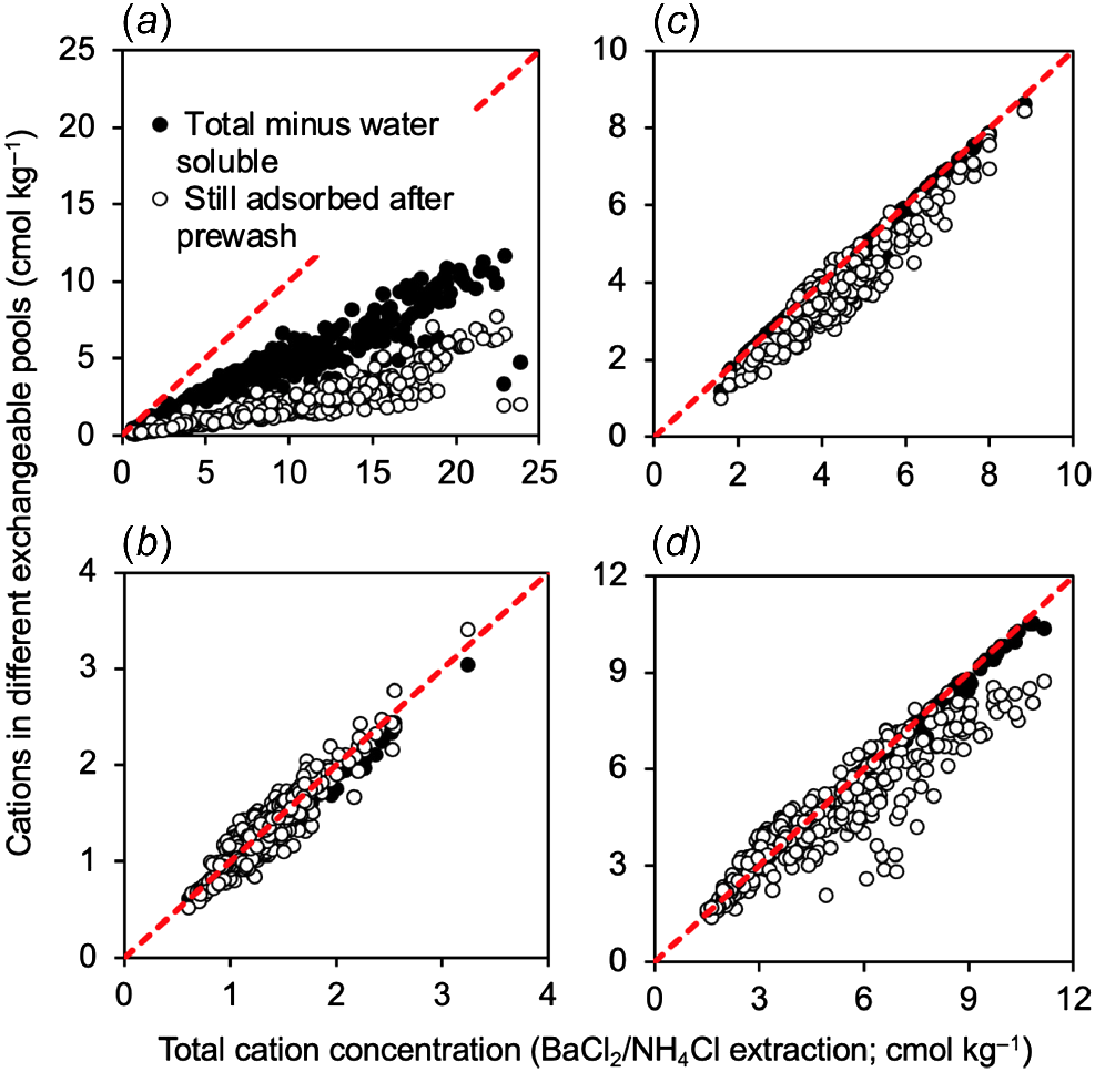
The results show that the two methods (use of alcohol pre-wash or difference between BaCl2/NH4Cl extract and soluble extract) gave similar results for K+ and Mg2+, somewhat different results for Ca2+ but very different results for Na+. For Na+ there was a divergence between the two groups of points across the entire range of total cation concentration tested (Fig. 1a). The result indicates that the use of the alcohol pre-wash stripped about 50% of the adsorbed Na+ from the exchange surfaces of the clay. For Ca2+ there was a divergence between the two groups of points particularly at moderate to high (8–12 cmol kg−1) total cation concentrations (Fig. 1d), indicating that the use of the alcohol pre-wash stripped Ca2+ from exchange surfaces at high total Ca2+ concentrations. By contrast, for K+ and Mg2+, the points for the pre-wash and the difference between BaCl2/NH4Cl extract and soluble extract largely overlayed each other (Fig. 1b, c).
Another issue that can be seen from Fig. 1 is that for K+, Mg2+ and Ca2+ the black-filled points (total minus soluble) fell close to the 1:1 line (dashed line) showing that total cations (x-axis) were nearly all in the adsorbed pool (y-axis) (Fig. 1b–d). However, this was not the case for Na+ (Fig. 1a). Here the black filled points (total minus soluble; y-axis) were approximately half the values on the x-axis, showing that about half the Na+ was in the adsorbed pool and the other half was soluble.
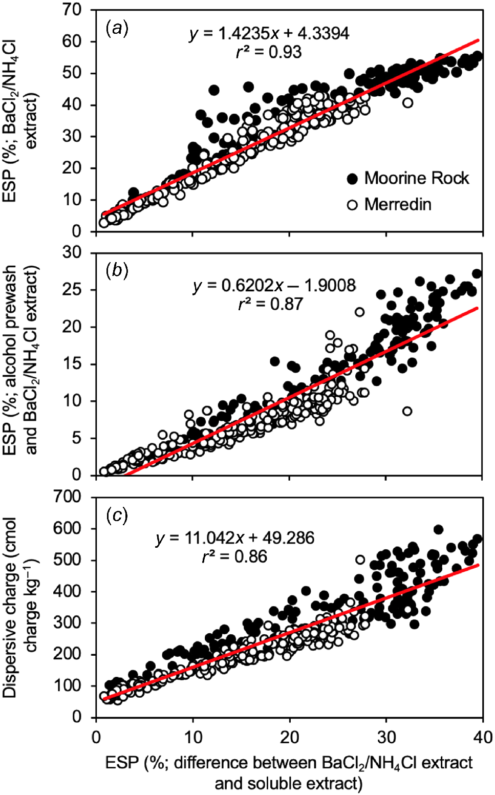
Fig. 2 shows several relationships between different methods of quantifying sodicity. For each of the three graphs, the x-variable is the ESP based on the truly adsorbed cations (BaCl2/NH4Cl extract minus soluble extract). In Fig. 2a, the x-variable was correlated with the ESP based on total cations (from the BaCl2/NH4Cl extract alone). The composite data set from Moorine Rock and Merredin produced a significant (P < 0.001) line of best fit with a slope of ~1.4, suggesting that about 40% of the Na+ in the BaCl2/NH4Cl extract was soluble. In Fig. 2b, the x-variable was correlated with the ESP based on the BaCl2/NH4Cl extract after alcohol pre-wash. The composite data set produced a significant (P < 0.001) line of best fit with a slope of 0.6, suggesting that about 40% of the exchangeable Na+ was lost because of the alcohol pre-wash. In Fig. 2c, the x-variable was correlated with dispersive charge (c.f. Rengasamy et al. 2016) also calculated based on the truly adsorbed cations (BaCl2/NH4Cl extract minus soluble extract). The composite data set from Moorine Rock and Merredin produced a significant (P < 0.001) line of best fit with a slope of ~11.
Relationships between ESP (based on difference between BaCl2/NH4Cl extract and soluble extract; x-variable) and either: (a) ESP based on BaCl2/NH4Cl extract alone (y-variable); (b) ESP based on alcohol pre-wash then BaCl2/NH4Cl extract (y-variable); or (c) dispersive charge (based on difference between BaCl2/NH4Cl extract and soluble extract; y-variable). Although different symbols have been used for data from Moorine Rock and Merredin, the lines of best fit have been drawn using composite data.
Given the outcomes of this section, we have calculated the ESP and dispersive charge assuming each exchangeable cation had to be determined as the total concentration (cmol kg−1 with a BaCl2/NH4Cl extract) minus the soluble concentration (cmol kg−1 with a water extract).
2. Characterising the soils: clay type, alkalinity, sodicity and salinity
A database of the soil physical and chemical variables measured on each soil sample is in the Supplementary Material, Tables S1 and S2. The analyses presented below show that the soils at the Moorine Rock and Merredin locations fell into two groups, which affected their alkalinity, sodicity, cation exchange capacity, and salinity.
X-ray diffraction spectrometry (XRD) and semi-quantitative analysis were used to determine the clay mineral concentrations for four soil samples from the soil layers (0–0.1 m and 0.4–0.5 m) at Moorine Rock and Merredin (trial ME11). Kaolinite was the dominant clay (66–91%) at each site and depth (Table 3). However, the secondary clays at Moorine Rock were vermiculite (8–16%) and illite (13% at 40–50 cm), whereas the secondary clay at Merredin was illite (29–34%). Vermiculite has a higher cation exchange capacity (100–150 mmol of charge per 100 g) than illite and kaolinite (10–40 and 3–15 mmol of charge per 100 g, respectively; Grim 1968).
| Location | Depth (m) | Clay minerology (%) | |
|---|---|---|---|
| Moorine Rock | 0–0.1 | Kaolinite (91%), vermiculite (8%) | |
| 0.4–0.5 | Kaolinite (71%), vermiculite (16%), illite (13%) | ||
| Merredin (ME11) | 0–0.1 | Kaolinite (66%), illite (34%) | |
| 0.4–0.5 | Kaolinite (71%), illite (29%) |
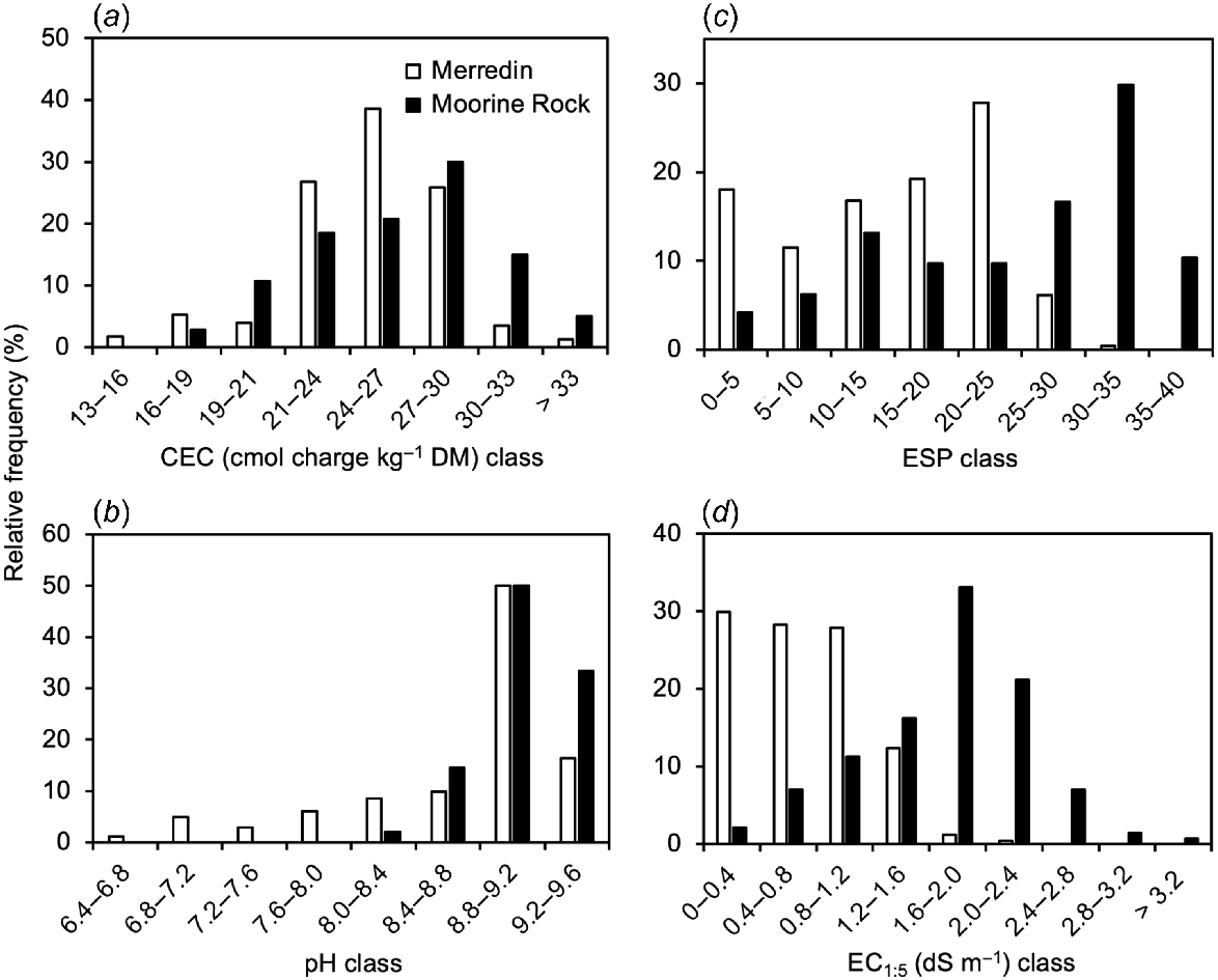
While a wide range of variables were measured (Supplementary material), variation in cation exchange capacity, pH, sodicity (ESP) and salinity were pivotal. Fig. 3 shows the relative frequency distribution of these four variables at Merredin and Moorine Rock, and Fig. 4 shows the variation in these four variables with average soil depth.
Relative frequency distribution of variation in four soil variables: (a) cation exchange capacity (CEC); (b) pH; (c) exchangeable sodium percentage (ESP); and (d) EC1:5. The data from Merredin and Moorine Rock were separated into different categories.
Variation in four soil variables with average depth in the soil profile: (a) cation exchange capacity; (b) pH; (c) exchangeable sodium percentage; and (d) EC1:5. Each point is the mean of 4–32 replicates. Error bars denote the standard error of the mean. Soils were from Moorine Rock or Merredin; the legend refers to the experiment numbers for the Merredin-based trials (see Table 1).
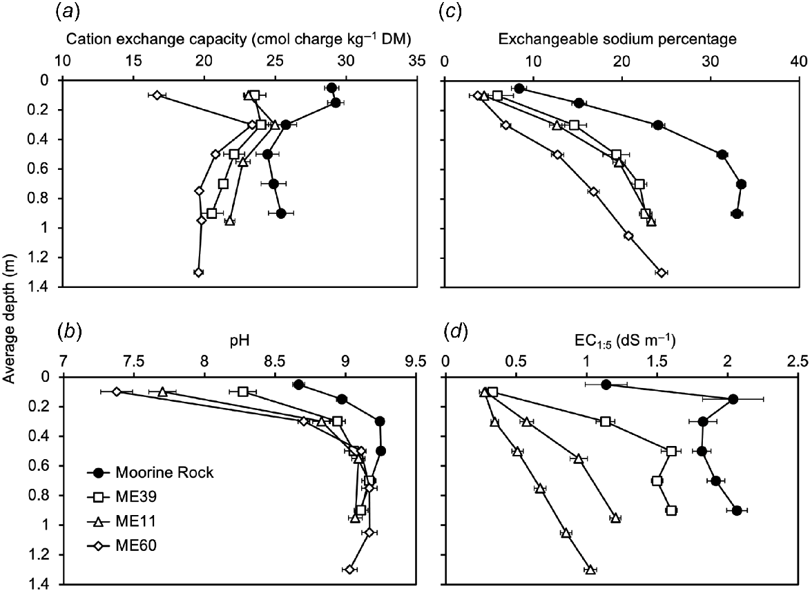
Relative frequency data showed that while the soils from each site had a wide range of CEC values, the soils from Moorine Rock reached higher values (median CEC = 27; 5th−95th percentile = 20–33 cmol charge kg−1 DM) than the soils from Merredin (median CEC = 25; 5th−95th percentile = 18–30 cmol charge kg−1 DM) (Fig. 3a). Average CEC values were higher at Moorine Rock than Merredin at all soil depths sampled. However, these differences were particularly pronounced at shallow depths. At average depths of 0.05 and 0.15 m average CEC values at Moorine Rock were at least 5 cmol charge kg−1 higher than for shallow depth soils at Merredin (Fig. 4a).
Relative frequency data showed that the soils from Moorine Rock had a more alkaline distribution (median pH = 9.1; 5th−95th percentile = 8.6–9.4) than the soils from Merredin (median pH = 9.1; 5th−95th percentile = 7.1–9.3) (Fig. 3b). Data collected across soil depths showed that lowest average pH values (8.7 for Moorine Rock, 7.4–8.3 for Merredin) occurred in surface soils, and highest average pH values (9.0–9.3) occurred at average depths of 0.5–1.05 m (Fig. 4b).
The severity of sodicity is indicated here as exchangeable sodium percentage (Figs 3c, 4c) and as dispersive charge (Supplementary material, Fig. S1). Relative frequency data showed that the soils from Moorine Rock had a more sodic distribution (median ESP = 28; 5th−95th percentile = 6–37) than the soils from the Merredin locations (median ESP = 16; 5th−95th percentile = 2–25) (Fig. 3c). Regarding depth effects (Fig. 4c) lowest average ESP values (4–8) occurred in the shallowest soil samples. At Moorine Rock, the highest average ESP value (33) occurred at an average depth of 0.7 m. However, for the three Merredin locations, the highest average ESP values (21–24) occurred at the deepest depths (average 0.9–1.3 m) sampled (Fig. 4c).
The general trends for dispersive charge were similar to exchangeable sodium percentage (Supplementary material, Fig. S1). For Moorine Rock, dispersive charge values ranged from 163 to 528 cmol charge kg−1, whereas for Merredin dispersive charge values were lower, ranging from 75 to 303 cmol charge kg−1 (5th−95th percentile in each case) (Supplementary material, Table S2a). Lowest average dispersive charge values (80–189 cmol charge kg−1) occurred at the shallowest depths sampled, and the highest average dispersive charge values (259–437 cmol charge kg−1) occurred at average depths of 0.9–1.3 m (Supplementary material, Fig. S2b).
The severity of salinity was indicated by the EC1:5. Relative frequency data showed that the soils from Moorine Rock were more saline (median EC1:5 = 1.8 dS m−1; 5th−95th percentile = 0.7–2.7 dS m−1) than the soils from the Merredin locations (median EC1:5 = 0.7 dS m−1; 5th−95th percentile = 0.2–1.5 dS m−1) (Fig. 3d). At all locations, lowest average EC1:5 values (0.3–1.1 dS m−1) occurred in the surface soil (Fig. 4d). At Moorine Rock, the highest average EC1:5 value (2.0 dS m−1) occurred at the second depth (average 0.15 m) sampled. By contrast for the four Merredin locations, the highest average EC1:5 values (1.0–1.6 dS m−1) occurred at the deepest depths (average 0.9–1.3 m) sampled (Fig. 4d).
3. EC1:5 increases mostly because of one soluble cation (Na+) and four soluble anions (Cl−, SO42−, HCO3−, and CO32−)
This section examines the degree to which EC1:5 was affected by and correlated with the concentrations of soluble cations and anions (Fig. 5).
Relationships between EC1:5 and soluble ion concentrations: (a) Na+, K+, Ca2+ and Mg2+; (b) Cl− and SO42−; and (c) HCO3− and CO32−. The indicated lines of best fit for Na+, Cl−, SO42−, and HCO3− were all significant at P < 0.001.
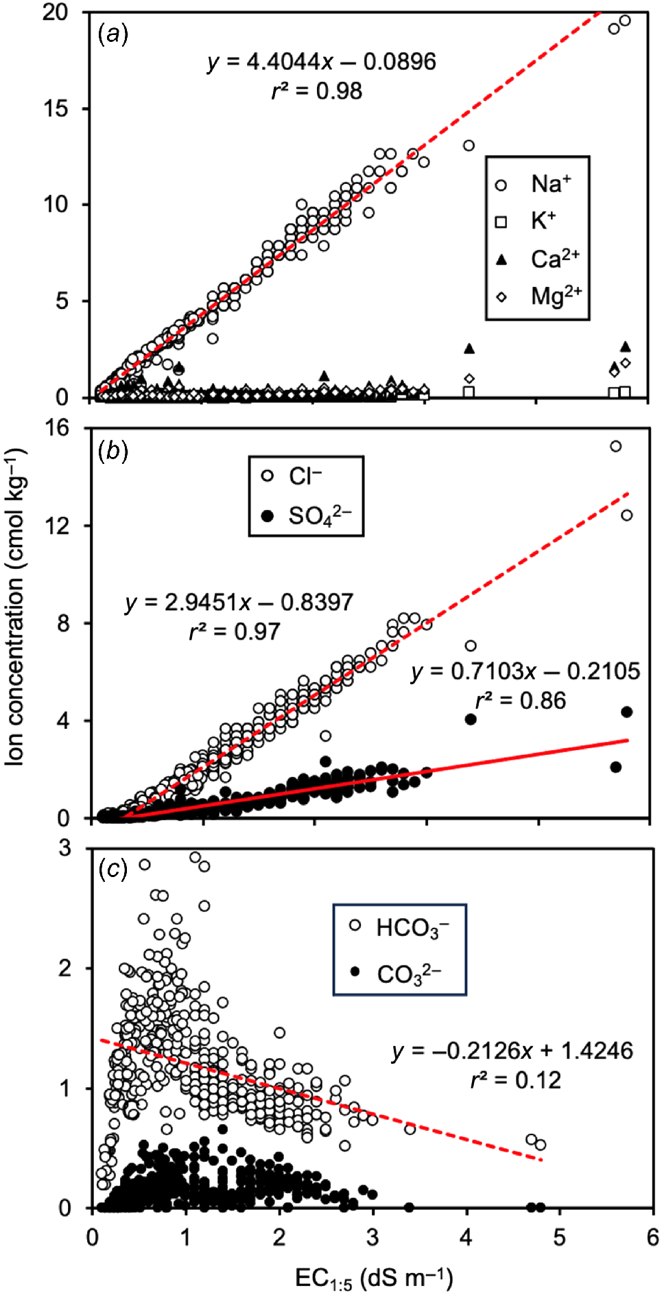
A useful quality assurance test for datasets like ours is to determine whether the sum of charge from soluble cations equals the sum of charge from soluble anions. The correlation of these two variables was significant (P < 0.001; r2 = 0.986) with a slope close to 1.0 (0.92; see Supplementary material, Fig. S3). We are therefore relatively confident that our methods adequately accounted for the cations and anions that could be extracted in water.
Of the soluble cations measured (Na+, K+, Ca2+, and Mg2+), Na+ was the most common cation. Across all soil samples analysed, Na+ accounted for the greatest proportion (55–98%; 5th−95th percentile) of the total soluble cation charge). The concentration of soluble Na+ was significantly positively correlated with the EC1:5 (P < 0.001; r2 = 0.984; Fig. 5a). No other soluble cation was correlated with EC1:5. Soluble Na+ was clearly the dominant cation causing high EC1:5 values.
Total anion charge was affected by all four soluble anions measured (Cl−, HCO3−, SO42− and CO32−). Table 4 shows the concentration of these averaged across each soil profile and the proportion of the total anion charge due to each. On average Cl−, HCO3−, and SO42− accounted for 33–61, 12–41%, and 16–28% of total anion charge, respectively, with the balance (3–10%) coming from CO32−.
| Location (depth) | Average concentration in profile (cmol kg−1) | Ratios | |||||||
|---|---|---|---|---|---|---|---|---|---|
| Na+ | Cl− | SO4 2− | HCO3 − | CO3 2− | Cl−/Na+ | SO4 2−/Na+ | HCO3 −/Na+ | ||
| Moorine Rock (0–1 m) | 8.20 | 4.57 | 1.14 | 1.01 | 0.21 | 0.56 | 0.14 | 0.12 | |
| ME39 (0–1 m) | 5.44 | 3.26 | 0.53 | 0.92 | 0.07 | 0.60 | 0.10 | 0.17 | |
| ME11 (0–1.2 m) | 3.70 | 1.61 | 0.36 | 1.31 | 0.15 | 0.44 | 0.10 | 0.35 | |
| ME60 (0–1.4 m) | 2.31 | 1.06 | 0.26 | 1.35 | 0.17 | 0.46 | 0.11 | 0.58 | |
| Average all sites | 4.92 | 2.52 | 0.60 | 1.20 | 0.17 | 0.51 | 0.12 | 0.24 | |
The values reported here are a weighted average by the proportion of the soil weight at each depth interval.
The concentrations of Cl− and SO42− were both significantly positively correlated with the EC1:5 (P < 0.001; r2 values 0.969 and 0.857, respectively; Fig. 5b). Interestingly, while the EC1:5 was affected by high HCO3−, these values were negatively correlated with HCO3− (P < 0.001; r2 = 0.124; Fig. 5c).
At Moorine Rock and Merredin site ME39, Cl− was the dominant anion, accounting for 55–60% of the anionic charge in the soil profile, with SO42− being of secondary significance (accounting for 20–28% of anionic charge). By contrast, at the other two Merredin locations (ME11 and ME60) Cl− and HCO3− were of comparable importance (each with 33–41% of the anionic charge).
4. Cause of high EC1:5 values: sodicity
Given the high pH, sodicity and EC1:5 (Fig. 4) that occurred in these soils, it was appropriate to determine whether the evidence pointed to high EC1:5 values being caused by variation in soil sodicity (or related variables) and/or pH.
Simple linear regression was conducted to determine the effects of a range of variables on EC1:5 using data aggregated across all sites (results summarised in Table 5). Initial results showed that the incorporation of data from shallow soils added strongly to the residuals in correlations. Therefore, Table 5a shows results for samples from depths greater than 0.2 m and Table 5b shows results for samples from all depths. In both situations, EC1:5 was most strongly positively correlated with variables indicative of increasing sodicity (dispersive charge, exchangeable Na+ and ESP; adj R2 values = 65–73% in Table 5a, and 46–59% in Table 5b). EC1:5 was also negatively correlated with exchangeable Ca2+ (adj. R2 = 48% in Table 5a, and 17% in Table 5b). The relationship incorporating pH was significant but was not as strong as for other variables (adj. R2 = 6% in Table 5a, and 20% in Table 5b).
| (a) Soil samples deeper than 0.2 m (n = 288) | |||
|---|---|---|---|
| Variable | Adj. R2 | Line of best fit | |
| Dispersive charge (DC; cmol charge kg−1) | 72.6 | EC1:5 = 0.004797 DC − 0.1490 | |
| Exchangeable Na+ (cmol kg−1) | 71.8 | EC1:5 = 0.22691 Na+ + 0.0475 | |
| ESP | 64.7 | EC1:5 = 0.06082 ESP − 0.1268 | |
| Exchangeable K+ (cmol kg−1) | 59.0 | EC1:5 = 1.7195 K+ − 0.850 | |
| Exchangeable Ca2+ (cmol kg−1) | 48.3 | EC1:5 = −0.2848 Ca2+ + 2.3479 | |
| Exchangeable Mg2+ (cmol kg−1) | 45.0 | EC1:5 = 0.4060 Mg2+ − 0.565 | |
| CEC (cmol charge kg−1) | 18.1 | EC1:5 = 0.07871 CEC − 0.606 | |
| pH1:5 | 5.6 | EC1:5 = 0.594 pH − 4.18 | |
| (b) Soil samples from all depths (n = 388) | |||
|---|---|---|---|
| Variable | Adj. R2 | Line of best fit | |
| Dispersive charge (DC; cmol charge kg−1) | 58.8 | EC1:5 = 0.004808 DC − 0.0785 | |
| Exchangeable Na+ (cmol kg−1) | 56.0 | EC1:5 = 0.21565 Na+ + 0.194 | |
| ESP | 45.8 | EC1:5 = 0.05069 ESP + 0.2026 | |
| Exchangeable Mg2+ (cmol kg−1) | 34.6 | EC1:5 = 0.3911 Mg2+ − 0.496 | |
| pH1:5 | 19.7 | EC1:5 = 0.5745 pH − 3.955 | |
| CEC (cmol charge kg−1) | 17.0 | EC1:5 = 0.07562 CEC − 0.649 | |
| Exchangeable Ca2+ (cmol kg−1) | 16.5 | EC1:5 = −0.1458 Ca2+ + 1.8305 | |
| Exchangeable K+ (cmol kg−1) | 15.1 | EC1:5 = 0.829 K+ + 0.061 | |
All relationships were significant at P < 0.001.
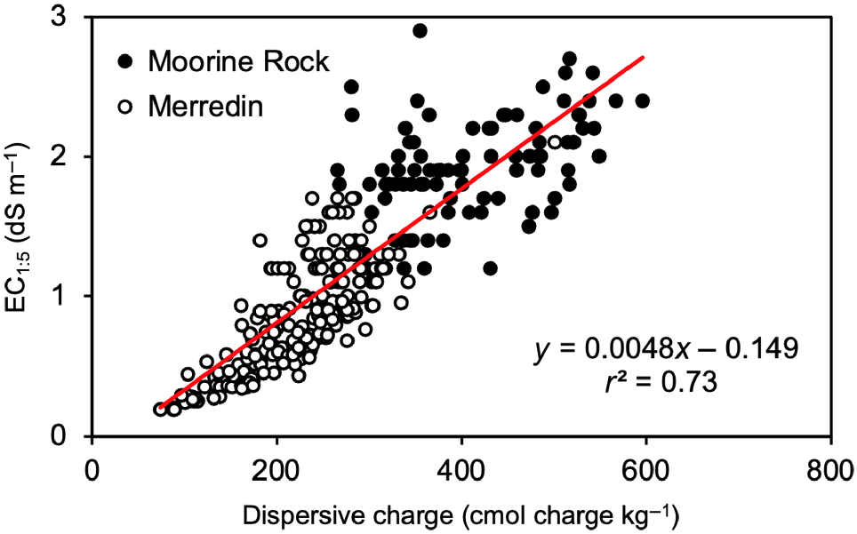
Fig. 6 shows a scatter-graph of the most significant positive relationship, that between EC1:5 (y-variable) and dispersive charge (x-variable) for soil samples deeper than 0.2 m, with those from Moorine Rock and Merredin indicated by different symbols. Despite the differences in clay mineralogy, the points from Moorine Rock and Merredin appeared to be co-linear and well-described by the line drawn in common between all points. Based on the line of best fit, EC1:5 values of 1, 2, and 3 dS m−1 occurred with dispersive charge values of ~240, 450, and 660 cmol charge kg−1 of soil, respectively.
5. Impacts of salts on osmotic potential
Fig. 5 shows that the bulk of the salinity hazard in these soils occurs because of the presence of NaHCO3, NaCl and Na2SO4, with Na2CO3 making up a small proportion of the total. Each of these salts is highly soluble, which means that their concentrations in the soil solution can be estimated from their concentrations in 1:5 soil:water extracts (c.f. Table 2). It also means that their contribution to the soil osmotic potential (Ψs) can be calculated based on previously determined relationships between each salt and Ψs (c.f. Wolf et al. 1986).
Osmotic potentials were estimated based on four assumptions. First, the osmotic potential of each soil sample was due to the presence of four anions: (1) Cl−; (2) SO42−; (3) HCO3−; and (4) CO32−, with Na+ as cation (Fig. 5). Second, the four sodium salts of these anions were dissolved either in the soil water content at the time of drilling or in a standard amount of water (30% soil dry weight). Third, the osmotic potential due to each salt could be calculated based on relationships derived from the data of Wolf et al. (1986). Fourth, total osmotic potential was the sum of the osmotic potentials of each individual component salt
Prior to sampling (in July 2022), the soils at Moorine Rock and Merredin received between ~65 mm and 69 mm of rain in May–June, respectively (based on nearby Bureau of Meteorology rainfall stations). With this early season rain, the soils at Moorine Rock contained an average of 11–14% gravimetric water in the upper 0.2 m of the soil profile, and 14–17% water in the deeper soil. The soils from Merredin contained an average of 13–18% water in the upper 0.2 m of the soil profile, and 12–17% water in the deeper soil (Fig. 7a).
Variation in gravimetric soil water content and osmotic potential with average depth in the soil profile: (a) soil water content at the time of sampling; (b) osmotic potential estimated assuming the soil water content of (a); and (c) osmotic potential estimated assuming a gravimetric soil water content of 30%. Each point is the mean of 4–32 replicates. Error bars denote the standard error of the mean. Soils were from Moorine Rock or Merredin; the legend refers to the experiment numbers for the Merredin-based trials (see Table 1).

Soil osmotic potentials in the different soil layers were estimated assuming that the salts were either dissolved in the soil water described above (Fig. 7b) or were dissolved in the water of soils hydrated to 30% moisture (Fig. 7c). The relative frequency of osmotic potentials was also determined for soil samples from the surface (0–0.2 m) and subsoil at Merredin and Moorine Rock; here the soils were separated into four categories with osmotic potentials between 0 and −0.5 MPa, −0.5 and −1.0 MPa, −1.0 and −1.5 MPa, and less than −1.5 MPa. (Fig. 8). For crops, osmotic potentials less than −0.5 MPa are likely to jeopardise the production of an economic yield (see Discussion).
Relative frequency distribution of osmotic potentials for Merredin and Moorine Rock at two levels of soil water content: the low water contents at sampling (a, c); and 30% gravimetric soil moisture (b, d). The data have been categorised according to soil depth: surface soil is at 0–0.2 m; subsoil is at depths >0.2 m.
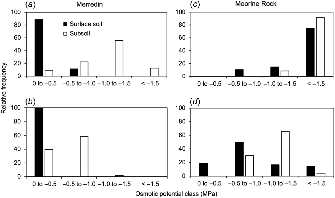
When osmotic potentials were calculated based on the water content at the time of sampling, there was strong stratification of osmotic potentials at Merredin (less negative in the surface soil, more negative in the subsoil) (Fig. 7b). At Merredin, most (88%) surface soil samples had osmotic potentials between 0 and −0.5 MPa, but there were few (only 9%) of subsoil samples in this class. Most (56%) subsoil samples had osmotic potentials between −1.0 and −1.5 MPa (Fig. 8a). By contrast, at Moorine Rock this stratification was not evident (Fig. 7b). Most surface soils (75%) and subsoils (92%) had osmotic potentials less than −1.5 MPa, and there were no soil samples in either depth range in the least severely affected class (from 0 to −0.5 MPa) (Fig. 8c).
Increasing soil water content to 30% made osmotic potentials less negative (Fig. 7c) which affected the distribution of soil samples across osmotic potential classes. At Merredin, the stratification of osmotic potential with depth was still evident (Fig. 7c), but 100% of surface soils were in the least severely affected class (from 0 to −0.5 MPa); there there were many (40%) subsoil samples in this class, but most (58%) subsoil samples were in the class from −0.5 to −1.0 MPa (Fig. 8b).
For Moorine Rock, increasing soil water content had a strong effect on the distribution of samples by osmotic potential (Figs 7c, 8d). In the surface soil, some (19%) samples were in the least severely affected class (from 0 to −0.5 MPa) and many (50%) were in the next class (from −0.5 to −1.0 MPa). However, the subsoil was still strongly osmotically affected with most samples (66%) in the class from −1.0 to −1.5 MPa (Fig. 8d).
Discussion
This paper has advanced the understanding of salinity and its causes in Calcarosols in Western Australia. Our work compared two Calcarosol soil profiles, in which kaolinite was the dominant clay species and illite also occurred in the subsoil. However, at Moorine Rock the soils also contained vermiculite, a clay mineral with a particularly high cation exchange capacity (100–150 cmol charge kg−1) compared with kaolinite and illite (3–15 and 10–40 cmol charge kg−1, respectively; Grim 1968); these soils were generally more sodic, alkaline and saline than those from Merredin.
Our work has four principal conclusions: (1) it provides further support to the case that the calculation of exchangeable cations in soils affected by salinity is best made by subtracting cations in the soluble extract from those in the total (BaCl2/NH4Cl) extract; (2) we have shown that the salinity in these sodic occurs because of the presence of Na+, Cl−, HCO3−, and SO42−; (3) salinity (particularly in subsoils) is most strongly associated with high dispersive charge (a variable recently developed for quantifying sodicity; c.f. Rengasamy et al. 2016) and by alkalinity; and (4) this form of salinity can strongly impact on soil osmotic potential. These four points will be discussed further below.
Measurement of exchangeable cations in soils affected by salinity
The idea that special care needs to be taken in the measurement of exchangeable cations in soils affected by salinity is not particularly new, but this key message is frequently ignored. Bower et al. (1952) proposed that exchangeable cations be determined from the difference between total cations (determined in an ammonium acetate extract) and soluble ions (determined in a saturation extract), and this approach was then widely promoted through USDA Handbook 60 (United States Salinity Laboratory Staff 1954). More recently, this case has been remade for Australia by So et al. (2006) using clay soils from Queensland with dominant clay species smectite and kaolinite.
The erroneous inclusion of soluble Na+ into the exchangeable component can have adverse consequences for the classification of soils. In the present work, using soils with EC1:5 values between 0.1 and 19.6 dS m−1 we found that the use of BaCl2/NH4Cl extractions over-represented adsorbed Na+ by ~50% (Fig. 1). This had consequences for the assessment of sodicity, exaggerating values of ESP by ~40% (see slope of line of best fit in Fig. 2a).
When ESP was calculated based on total cations after alcohol pre-wash, values were ~40% lower than when calculated with the truly adsorbed cations (i.e. BaCl2/NH4Cl extract minus soluble extract) (see slope of line of best fit in Fig. 2b). This shows that about 40% of the truly adsorbed Na+ is weakly held on the exchange surfaces of the clay and is easily leached off. A similar conclusion was reached by So et al. (2006).
In their seminal work ‘Australian soils with saline and sodic properties’, Northcote and Skene (1972) proposed that sodic soils in Australia should be defined as having ESP values >6 and highly sodic soils should be defined as having ESP values >15. At the present time, there are no published critical values defining sodic and highly sodic soils based on dispersive charge. It is unclear whether the original Northcote and Skene assessment was made using soils affected by salinity, but if we take their critical values for ESP at face value then our correlation between ESP and dispersive charge (Fig. 2c) suggests that the critical dispersive charge limit could be 115 cmol charge kg−1 for ‘sodic’ soils and 215 cmol charge kg−1 for ‘highly sodic’ soils (c.f. Fig. 2c). It would be useful to see these values confirmed using reliable ESP and dispersive charge data from other regions.
Ions causing salinity
One feature of our dataset is the diversity of ions responsible for salinity (Na+, Cl−, HCO3−, SO42−, CO32−). Because Cl− is the dominant anion in seawater (accounting for ~90% of the anionic charge; Lyman and Fleming 1940), there has been a tendency to think that Cl− should be the dominant anion in saline soils in Australia. Our dataset shows that this should not be assumed. HCO3− was at higher concentrations than Cl− in 167 (43%) of the 388 soil samples measured (see Supplementary material Table S2).
Causes of salinity
Our data lead us to suggest that there are three drivers of salinity in Calcarosols: (1) sodicity decreases the permeability of the soils, resulting in the accumulation of salts from rainfall and the atmosphere; (2) soil alkalinity leads to increased bicarbonate and carbonate; and (3) soil salinities are impacted by rainfall and evaporation.
The results summarised in Table 5 provide strong evidence supporting the view that the principal cause of salinity is sodicity: an adjusted R2 of 72.6% for the relationship between EC1:5 and dispersive charge (Table 5a and Fig. 6) leaves little room for doubt. We presume that high sodicity causes soil dispersion and the loss of soil porosity; this decreases soil saturated hydraulic conductivity (Ks) by orders of magnitude so that salt deposited on the soil as aerosols or in the rain leaches into the soil extremely slowly; this salt therefore accumulates (c.f. Rengasamy 2002). The scale of the impact of sodicity on Ks can be seen in studies in which sodicity is reversed. For example, in an alkaline sodic soil with a Ks of 0.0007 m h−1, the reversal of sodicity through the application of gypsum increased Ks to 0.26 m h−1, a 370-fold increase (Chorom and Rengasamy 1997).
The soils examined here are deeply weathered and if the ions in the profiles had accumulated from rainfall (a plausible hypothesis; c.f. Rengasamy 2002; Barrett-Lennard et al. 2016), then this must have occurred over tens of thousands of years. According to Hingston and Gailitis (1976), the rain at 250–330 km from the west coast of WA contains about ~4 mg L−1 Cl−. Given this, the Cl− concentrations reported for the upper 1–1.4 m of our soil profiles (Table 4) would have required a period to accumulate of at least 23,000 years for Moorine Rock and 7,000–15,000 years for the three locations at Merredin (assuming no salt leaching). These estimates were calculated assuming that average rainfall at Moorine Rock and Merredin is 303 and 325 mm per year, respectively (Bureau of Meteorology 2024), the rain contains 4 mg Cl− L−1 (Hingston and Gailitis 1976), and the soils have a bulk density of ~1.7 Mg m−3 (Moore 2001). One of the interesting features of the data in Table 4 is that the ratio of soluble Cl−/Na+ is substantially less than 1:1 (the ratio of these ions in seawater). We presume that this occurs partly because Cl− is more leachable in these soils than Na+ but also because a large proportion of the anionic composition of the soil comes from the presence of HCO3− and CO32−, and that this is an inevitable consequence of alkalinity.
A second point arising from Table 5 is that the weaker (but still highly significant) relationships between EC1:5 and pH are consistent with the view that alkalinity is an additional factor contributing to salinity. Meta-analyses of soil data at global scale show that alkaline soils predominantly occur in areas where mean annual evapotranspiration exceeds mean annual rainfall (Slessarev et al. 2016). Alkalinity causes bicarbonate and carbonate to increase in soils (Hassett 1973; see Supplementary material, Appendix S1), and these ions together accounted for 10–88% of the soluble anionic charge (5th−95th percentile) in our soils.
Table 5 also shows that EC1:5 values are affected by depth in the soil profile, with shallow soils being less rigorously ‘regulated’ by sodicity than deeper soils. This suggests that surface salinity is also affected by local weather conditions, i.e. higher salinities may occur in surface soils in summer due to capillarity, and lower salinities may occur in surface soils in winter due to the leaching effects of rain.
Impacts on osmotic potential
Salt affects crop growth for two major reasons: (1) adverse effects on plant water relations; and (2) specific ion effects (i.e. toxicities) that directly adversely affect cell metabolism (Greenway and Munns 1980; Munns and Tester 2008). The former effects occur because salinity decreases the osmotic potential of the soil solution; this lowers the water potential of the soil and places plants under osmotic stress. The latter effect occurs because, when taken up, the ions adversely affect metabolism. For example, Na+ can adversely affect many of the metabolic functions in plants that are normally facilitated by K+ (Munns and Tester 2008; Shabala and Cuin 2008).
Total water potential is the sum of the soil’s osmotic potential (Ψs) and matrix potential (Ψm), both negative numbers. At the water contents reported in Fig. 6a, Ψm values would presumably also have been low (negative) but we are not able to quantify these effects using our data. However, we can calculate Ψs values using soil ion concentration and water content measurements, which provides a sense of the magnitude of crop water stress.
What do the osmotic potential values reported in Figs 7 and 8 mean for crop growth? Published data (Maas and Hoffman 1977; Steppuhn et al. 2005a, 2005b) suggest that the yields of most crops can be expected to become unprofitable as osmotic potentials decrease from 0 to −0.5 MPa and plant survival will be threatened at more negative osmotic potentials. In addition, osmotic potentials in the range from 0 to −0.5 MPa can substantially decrease germination (for our summary see Supplementary material, Appendix S2). We conclude that for grain crops in Australia, profitability will be negligible at osmotic potentials less than −0.5 MPa.
In this work, we have calculated soil osmotic potential (MPa) as the sum of the individual osmotic potentials due to NaCl, NaHCO3, Na2SO4, and Na2CO3. We need to ask whether there is there any point in doing this, or whether the results are about the same as would be achieved by multiplying the EC1:5 (dS m−1) by the dilution factor of the 1:5 extract relative to the soil (i.e. 500/W; Rengasamy 2010) and a general factor for converting EC to Ψs (i.e −0.036; Marschner 1995). We have compared the two methods of calculating osmotic potential in Supplementary material Fig. S4 for osmotic potentials calculated using the measured gravimetric soil water content in the soil (Fig. 7a). The correlation between the two methods had a slope of 1.07 and an r2 value of 0.98. This outcome supports the view that the two methods give similar results, and it might not be necessary to go to the trouble of measuring soluble anions for the estimation of osmotic potential in future work.
One of the strong messages from this paper is that higher soil water content is important in increasing (making less negative) osmotic potentials (c.f. Figs 7b, 8a, and c with low water content, and Figs 7c, 8b, and d with 30% soil moisture). At Moorine Rock, in surface soils osmotic potentials were occasionally greater (less negative) than −0.5 MPa with 30% soil water but were never greater than −0.5 MPa at low water content. By the contrast, the effects of moisture were less severe at Merredin. When osmotic potentials were calculated based on the soil water contents at sampling, osmotic potentials were mostly greater than −0.5 MPa in surface soils and were all greater than −0.5 MPa in surface soils with 30% soil moisture. However, this differed in the subsoil. With the soil water at sampling, most (~90%) of soil samples had osmotic potentials less than −0.5 MPa, and even with the higher level of soil moisture about 60% of soil samples had osmotic potentials less than −0.5 MPa (Fig. 8).
Three conclusions emerge from these data: (1) we can expect that crop growth at Moorine Rock will be severely affected by low osmotic potentials; (2) it is likely that crop rooting depths will be constrained by low osmotic potentials in subsoils at Merredin; and (3) the adverse effects of salinity will be more severe in dry than wet growing seasons.
We conclude with a final point. Our measurements of the salinity of the soil solution and osmotic potential have been estimated for the bulk soil. However, it needs to be acknowledged that in clayey soils plant roots will tend to grow mostly through macropores. Salt concentrations in the soil solutions lining macropores might differ from those of the bulk soil either because of accelerated leaching during periods of rainfall (c.f. Allaire et al. 2009), or because of salt accumulation in the root-zone caused by the mass flow of the soil solution to the root surface and the uptake there of water but not salt (c.f. Alharby et al. 2014). There is therefore a need for work to be conducted to examine the variation in estimated salinities in exposed soil faces at millimetre-scale paying particular attention to the salinity of the soil solution in massive peds and macropores.
Data availability
The data used in the writing of this paper have been tabled in the supplementary materials.
Declaration of funding
This research was conducted with the financial support of the Department of Primary Industries and Regional Development and the Grains Research and Development Corporation (Project DAW1902-001RTX).
Acknowledgements
The soil coring was conducted by Robert Courtney Bennett. We are grateful for the support of the staff of Merredin Research Station (Merredin) and to Glenn Nicholson (Moorine Rock) for their support of our trials. We are also grateful to Dr Paul Blackwell for thoughtful critique of this manuscript.
References
Alharby HF, Colmer TD, Barrett-Lennard EG (2014) Salt accumulation and depletion in the root-zone of the halophyte Atriplex nummularia Lindl.: influence of salinity, leaf area and plant water use. Plant and Soil 382, 31-41.
| Crossref | Google Scholar |
Allaire SE, Roulier S, Cessna AJ (2009) Quantifying preferential flow in soils: a review of different techniques. Journal of Hydrology 378, 179-204.
| Crossref | Google Scholar |
Barrett-Lennard EG, Anderson GC, Holmes KW, Sinnott A (2016) High soil sodicity and alkalinity cause transient salinity in south-western Australia. Soil Research 54, 407-417.
| Crossref | Google Scholar |
Bower CA, Reitemeier RF, Fireman M (1952) Exchangeable cation analysis of saline and alkali soils. Soil Science 73, 251-262.
| Crossref | Google Scholar |
Bureau of Meteorology (2024) Climate data on-line. Bureau of Meteorology. Available at www.bom.gov.au/climate/data
Chorom M, Rengasamy P (1997) Carbonate chemistry, pH, and physical properties of an alkaline sodic soil as affected by various amendments. Australian Journal of Soil Research 35, 149-161.
| Crossref | Google Scholar |
Frenkel H, Goertzen JO, Rhoades JD (1978) Effects of clay type and content, exchangeable sodium percentage, and electrolyte concentration on clay dispersion and soil hydraulic conductivity. Soil Science Society of America Journal 42, 32-39.
| Crossref | Google Scholar |
Greenway H, Munns R (1980) Mechanisms of salt tolerance in nonhalophytes. Annual Review of Plant Physiology 31, 149-190.
| Crossref | Google Scholar |
Hassani A, Azapagic A, Shokri N (2020) Predicting long-term dynamics of soil salinity and sodicity on a global scale. Proceedings of the National Academy of Sciences of the United States of America 117, 33017-33027.
| Crossref | Google Scholar |
Hassett J (1973) Equilibrium concepts in soil—the use of the CO2-H2O system in teaching equilibrium concepts. Journal of Agronomic Education 2, 68-72.
| Crossref | Google Scholar |
Hingston FJ, Gailitis V (1976) The geographic variation of salt precipitated over Western Australia. Australian Journal of Soil Research 14, 319-335.
| Crossref | Google Scholar |
LabXchange (2023) Solute potential: the formula. Available at https://www.labxchange.org/library/items/lb:LabXchange:77c13493:lx_image:1 [accessed 14 October 2024]
Lyman J, Fleming RH (1940) Composition of sea water. Journal of Marine Research 3, 134-146.
| Google Scholar |
Maas EV, Hoffman GJ (1977) Crop salt tolerance – current assessment. Journal of the Irrigation and Drainage Division, American Society of Civil Engineers 103, 115-134.
| Crossref | Google Scholar |
Miller WP, Miller DM (1987) A micro-pipette method for soil mechanical analysis. Communications in Soil Science and Plant Analysis 18, 1-15.
| Crossref | Google Scholar |
Munns R, Tester M (2008) Mechanisms of salinity tolerance. Annual Review of Plant Biology 59, 651-681.
| Crossref | Google Scholar | PubMed |
Nuttal JG, Armstrong RD, Connor DJ, Matassa VJ (2003) Interrelationships between edaphic factors potentially limiting cereal growth on alkaline soils in north-western Victoria. Australian Journal of Soil Research 41, 277-292.
| Crossref | Google Scholar |
Rengasamy P (2002) Transient salinity and subsoil constraints to dryland farming in Australian sodic soils: an overview. Australian Journal of Experimental Agriculture 42, 351-361.
| Crossref | Google Scholar |
Rengasamy P (2010) Soil processes affecting crop production in salt-affected soils. Functional Plant Biology 37, 613-620.
| Crossref | Google Scholar |
Rengasamy P, Tavakkoli E, McDonald GK (2016) Exchangeable cations and clay dispersion: net dispersive charge, a new concept for dispersive soil. European Journal of Soil Science 67, 659-665.
| Crossref | Google Scholar |
Shabala S, Cuin TA (2008) Potassium transport and plant salt tolerance. Physiologia Plantarum 133, 651-669.
| Crossref | Google Scholar | PubMed |
Slessarev EW, Lin Y, Bingham NL, Johnson JE, Dai Y, Schimel JP, Chadwick OA (2016) Water balance creates a threshold in soil pH at the global scale. Nature 540, 567-569.
| Crossref | Google Scholar | PubMed |
So HB, Menzies NW, Bigwood R, Kopittke PM (2006) Examination into the accuracy of exchangeable cation measurement in saline soils. Communications in Soil Science and Plant Analysis 37, 1819-1832.
| Crossref | Google Scholar |
Stavi I, Thevs N, Priori S (2021) Soil salinity and sodicity in drylands: a review of causes, effects, monitoring, and restoration measures. Frontiers in Environmental Science 9, 712831.
| Crossref | Google Scholar |
Steppuhn H, van Genuchten MTh, Grieve CM (2005a) Root-zone salinity: I. Selecting a product-yield index and response function for crop tolerance. Crop Science 45, 209-220.
| Crossref | Google Scholar |
Steppuhn H, van Genuchten MTh, Grieve CM (2005b) Root-zone salinity: II. Indices for tolerance in agricultural crops. Crop Science 45, 221-232.
| Google Scholar |
Teakle LJH, Burvill GH (1938) The movement of soluble salts in soils under light rainfall conditions. Journal of Agriculture of Western Australia 15, 218-245.
| Google Scholar |