QES-Fire: a dynamically coupled fast-response wildfire model
Matthew J. Moody A , Jeremy A. Gibbs B , Steven Krueger C , Derek Mallia C , Eric R. Pardyjak A , Adam K. Kochanski D , Brian N. Bailey E and Rob Stoll A *
A *
A Department of Mechanical Engineering, University of Utah, Salt Lake City, Utah, USA.
B National Oceanic and Atmospheric Administration/Oceanic and Atmospheric Research National Severe Storms Laboratory, Norman, Oklahoma, USA.
C Department of Atmospheric Sciences, University of Utah, Salt Lake City, Utah, USA.
D Department of Meteorology and Climate Science, San Jose State University, San Jose, California, USA.
E Department of Plant Sciences, University of California Davis, Davis, California, USA.
International Journal of Wildland Fire 31(3) 306-325 https://doi.org/10.1071/WF21057
Submitted: 30 April 2021 Accepted: 21 January 2022 Published: 18 March 2022
© 2022 The Author(s) (or their employer(s)). Published by CSIRO Publishing on behalf of IAWF. This is an open access article distributed under the Creative Commons Attribution-NonCommercial 4.0 International License (CC BY-NC)
Abstract
A microscale wildfire model, QES-Fire, that dynamically couples the fire front to microscale winds was developed using a simplified physics rate of spread (ROS) model, a kinematic plume-rise model and a mass-consistent wind solver. The model is three-dimensional and couples fire heat fluxes to the wind field while being more computationally efficient than other coupled models. The plume-rise model calculates a potential velocity field scaled by the ROS model’s fire heat flux. Distinct plumes are merged using a multiscale plume-merging methodology that can efficiently represent complex fire fronts. The plume velocity is then superimposed on the ambient winds and the wind solver enforces conservation of mass on the combined field, which is then fed into the ROS model and iterated on until convergence. QES-Fire’s ability to represent plume rise is evaluated by comparing its results with those from an atmospheric large-eddy simulation (LES) model. Additionally, the model is compared with data from the FireFlux II field experiment. QES-Fire agrees well with both the LES and field experiment data, with domain-integrated buoyancy fluxes differing by less than 17% between LES and QES-Fire and less than a 10% difference in the ROS between QES-Fire and FireFlux II data.
Keywords: buoyant plume, diagnostic wind solver, fire–atmosphere coupling, level set method, merging plumes, plume rise model, rate of spread, simplified fire spread physics.
Introduction
Winds are one of the primary drivers at the fire front (Albini 1982) dictating fire-spread behaviour. Currently, only models that directly include the physical coupling between combustion processes and fluid momentum and scalar transport represent this phenomenon with minimal parameterisation or empiricism. For wildfires, these include models such as FIRETEC (Linn et al. 2002), the Wildland–Urban Interface Fire Dynamics Simulator (WFDS, Mell et al. 2007) and Firestar (Morvan and Dupuy 2004; Morvan et al. 2009). These models resolve fire progression based on physical representation of the combustion without relying on rate of spread (ROS) parameterisations, and account for the impact of fire–atmosphere interactions on fire behaviour. These models directly resolve entrainment due to combustion, as well as buoyancy, by solving the equations for conservation of mass, momentum and energy. However, the resolution required to resolve the physics of atmosphere–fire interactions precludes simulations that cover a large enough range of spatial and temporal scales to represent large wildfires such as those that have transpired in recent years, e.g. the 2018 British Columbia wildfires, which burned 1 354 284 ha (BC Wildfire Services 2020), the 2020 Oregon wildfires, which burned more than 400 000 ha (National Interagency Fire Center (NIFC) 2020), and the August complex fire in California, which burned more than 417 000 ha (NIFC 2020).
One solution used to mitigate the high computational cost of full-physics models is to simplify and parameterise different components of the fire–atmosphere system, for example the ROS. For wildfire, this is commonly done with empirically derived parameterisations. One example is the Fire Area Simulator (FARSITE, Finney et al. 1995), a deterministic modelling system capable of simulating fire spread in heterogeneous terrain with heterogeneous fuel and fuel moisture conditions. It includes several semi-empirical ROS models: the Rothermel (1972) surface fire spread model, the Van Wagner (1977) crown fire initiation model, the Rothermel (1991) crown fire spread model, the Albini (1979) spotting model, and the Nelson (2000) dead fuel moisture model. Another example of an empirically parameterised model is the narrow-band Eulerian Level set Method of Fire spread (ELMFire, Lautenberger 2013). ELMFire includes the Rothermel (1972) surface fire spread model as the forcing of a level set method (Sethian 1999). Each point of the fire front is advanced by applying Huygens’ principle, which assumes that the fire front propagation can be approximated as the sum of elliptical wavelets emanating from each point of the fire front (Baker and Copson 2003). Models such as FARSITE and ELMFire represent fire behaviour with ingested meteorological data as the forcing, but are limited because fire heat sources do not affect atmospheric winds.
Models such as the Coupled Atmosphere–Wildland Fire Environment (CAWFE, Clark et al. 2004; Coen 2013), MesoNH-ForeFire (Filippi et al. 2011), Weather Research and Forecasting – SFIRE (WRF-SFIRE, Mandel et al. 2011, 2014), and WRF-Fire (Coen et al. 2013; Muñoz-Esparza et al. 2018) focus on the coupling between mesoscale meteorological conditions and wildfire behaviour at spatial scales of the order of hundreds of metres ( ) using numerical weather prediction (NWP) models. For example, WRF-SFIRE couples the WRF model (Skamarock and Klemp 2008) with semi-empirical ROS and simplified fire heat flux parameterisations. A level set method is used to track and advance the flame front, and winds from the WRF model are interpolated to the fire front height for use in the ROS and fuel consumption models. In turn, heat fluxes from SFIRE are injected into the WRF model as a vertically distributed flux using an extinction depth. MesoNH-ForeFire (Filippi et al. 2011, 2013) uses the model of Balbi et al. (2009) as a forcing to a Lagrangian front tracking scheme. The ForeFire module interpolates the atmospheric winds to the midflame height and then calculates the fire-induced winds through the heat and water vapour surface fluxes. These combined winds are used to drive the ROS model. The main differences in these models are in the methodology for how the winds are interpolated to the fire front, the choice of ROS parameterisation, and how the heat and mass fluxes are injected into the atmospheric model. The feedback between meteorological variables and fire heat and mass fluxes enables these models to simulate fire-related winds and wildfire evolution. Kochanski et al. (2013) demonstrated that WRF-SFIRE can run coupled atmosphere–fire simulations faster than real time for large-scale wildfires. The primary limitation is that the grid resolution for such fires must be fairly modest (
 (100 m)) to keep the computational time low enough for forecasting applications.
WRF-SFIRE and similar models use a full set of prognostic equations to represent the atmosphere in a coupled modelling framework, making them computationally intensive. They also typically use near-surface atmospheric and fire front-scale parameterisations that were not developed for the small-scale three-dimensional (3-D) heterogeneity commonly found in most ecosystems. Recently, a third approach has emerged to couple atmospheric flow to fire spread that attempts to bridge the gap between the FIRETEC-WFDS approach and the coupled mesoscale atmosphere-to-fire front approach. The basic idea is to employ a simplified but still 3-D physics methodology for the microscale flow while representing fire behaviour with parameterisations similar to those used by WRF-SFIRE. QUIC-fire (Linn et al. 2020) does this by combining the diagnostic wind solver QUIC-URB (Pardyjak and Brown 2003) with a cellular automata model (Achtemeier 2013). QUIC-fire improves on the cellular automata model to include a more physics-based approach. It moves ‘energy packets’ (EP) through diffusion or advection based on the local wind. The transferred EP is used to either start new fires, intensify fires already ignited, or transfer the energy to the environment using a probability-based ROS. In addition, the impacts of fluxes originating at the fire front on the wind field are parameterised in QUIC-fire by converting the heat flux at the fire source to a buoyant plume with the plume centreline vertical velocity and lateral expansion calculated using the Briggs theory parameterisations (Davidson 1989).
Here, we present a new fast-response microscale model for wildfire spread, QES-Fire. It shares some characteristics with QUIC-fire, including the use of a similar diagnostic wind model, and its general strategy is similar while the specific submodels, methods and system flow are unique. The model is based on the QES (Quick Environmental Simulation) framework, a fast-response microscale model that can rapidly calculate wind fields in complex terrain (Bozorgmehr et al. 2021). QES-Fire uses quasi-steady-state simplified physics parameterisations to dynamically couple the ROS and fire heat fluxes with local winds. We first describe the modelling methodology used to create QES-Fire in the next section, including the fire front advancement method, the microscale wind solver, the ROS model and the parameterisations for the fire-induced winds through use of a convective plume model. The convective plume model includes single axisymmetric plumes as well as a methodology for determining the criteria for plume merging. Next, we compare the model in the ‘QES-Fire comparison’ section against an idealised plume and in situ measurements from an experimental burn.
QES-Fire modelling methodology
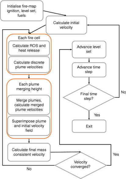
The goal of QES-Fire is to dynamically link near-surface atmospheric flow with fire front fluxes and fire front ROS in a physically consistent and computationally efficient manner. To accomplish this, a unique combination of reduced-order physical and chemical models, numerical methods and computational approaches is used. The model is composed of a set of linked submodels, each representing an aspect of the wildfire–atmosphere system (Fig. 1). Briefly, the coupling between atmospheric winds and fire heat fluxes is accomplished using a ROS model that advances the fire front through the level set method (Sethian 1999). The level set advances through QES-Fire’s discrete, two-dimensional (2-D) surface mapper that tracks fuel conditions at the domain’s surface. At the beginning of a simulation, the 2-D mapper is initialised with the fire’s ignition source and fuel characteristics. Next, an initial wind field is specified throughout the 3-D domain using QES-Winds and at each discrete cell that is on fire, a ROS model (Balbi et al. 2020) calculates the forcing used to advance the level set as well as the heat release of each discrete section of the fire front. A plume rise and merging model is then used to calculate a velocity field from the discrete fire map. The empirical plume velocity field is superimposed onto the initial velocity field and QES-Winds calculates a final velocity field. This iterates until convergence at which point the level set (fire front) and time step are advanced.
|
The following subsections give detailed descriptions of each component depicted in Fig. 1 and how they contribute to QES-Fire. All variables used in QES-Fire are listed in Table 1.

|
Fire map
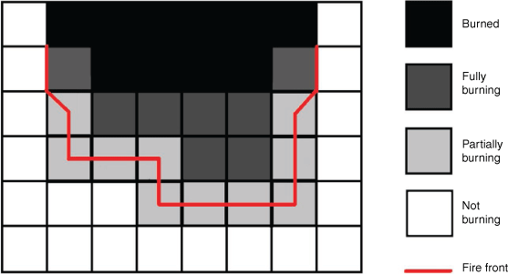
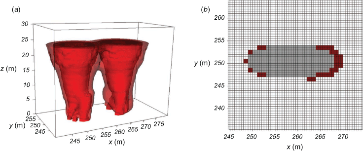
QES-Fire uses a cellular 2-D surface map to track fuels, moisture, local terrain slope and the fire front. All values are calculated at cell centres. The 2-D mapper (Fig. 2) defines four types of cells: not burning, partially burning, fully burning and burned. Additionally, the 2-D mapper tracks the fire front using the level set method (see ‘Fire front’ section). While the fire front is tracked as a continuous function (or set of continuous functions for multiple fires), each cell of the 2-D mapper is defined independently. Using a cellular approach gives QES-Fire the ability to build a fire front for heterogeneous conditions by varying the fuel loading, moisture and local slope for each distinct ground cell.
|
Fuel properties for each ground cell are specified according to the Rothermel (1972) and Anderson (1982) fuel loading models. These models include all the inputs necessary to compute the Rothermel ROS model. Each cell is considered homogeneous throughout; this is required because many ROS models assume a uniform fuel bed (e.g. Rothermel 1972; Pagni and Peterson 1973; Balbi et al. 2009). QES-Fire uses two ROS models concurrently to advance the fire front, Rothermel (1972) and Balbi et al. (2020) (see ‘Rate of spread model’ section below).
QES-Fire’s 2-D mapper uses the cell type to track where the fire front is in time and space. The ROS model calculates the ROS in all cells that are fully and partially burning and the fire front is advanced using a dynamic timestep (Δt) within all partially burning cells. Δt is calculated using a modified Courant number, C (Ferziger and Peric 2002), with the maximum ROS for the 2-D mapper replacing the velocity magnitude

where C ≤ 1. The ROS-dependent timestep ensures that the flame front does not skip cells, facilitating an accurate calculation of the time on fire (t) through a simple addition of Δt to the current time on fire. At the point in time when t ≥ τ, where τ is the residence time calculated based on the fuel type and moisture following Anderson (1969), the cell is considered burned out and the cell type is set to burned so that fire cannot re-spread to that cell.
Fire front
The fire front is advanced through the level set method described by Sethian (1999). The level set method was chosen for its ability to track a fast-evolving interface in complex geometries, and because it has been shown to be adept at fire front tracking (e.g. Mallet et al. 2009; Rehm and McDermott 2009; Mandel et al. 2011; Muñoz-Esparza et al. 2018). The initial fire front is prescribed in the initialisation of QES-Fire as the level set function ϕ so that ϕi,j(t = 0) = 0, where ϕi,j = 0 are burning cells and the subscripts i and j indicate the cell index in the x and y directions, respectively. A signed distance function (the minimum distance from a point to the level set) is then applied to all cells to determine the initial values for ϕ. Ghost cells are used by copying the values of the level set at the fire map boundaries to a buffer region around the 2-D mapper. This ensures spatial derivatives are non-complex at domain boundaries. As the progression is always forwards in a fire front (a fire cannot burn where it has already burned), it is appropriate to use an upwind numerical scheme; therefore, a first-order space convex scheme is utilised where

with Δt calculated using the modified Courant number (Eqn 1). Fi,j is the level set forcing function given by the ROS model (see ‘Rate of spread model’ section) and  and
and  are the forward and backward gradients (in space) of the level set calculated by

and

respectively. The level set spatial derivatives Di,j are given by


The level set forcing function Fi,j must be applied normal to the fire front, both in calculation of the ROS and for the propagation of the level set itself. The level set normal is calculated as

with

and

where nx and ny are the x and y components of the level set normal, respectively.
Microscale winds
The QES modelling framework is used to dynamically couple the fire front ROS and the velocity field using QES’s 3-D diagnostic wind solver QES-Winds (Bozorgmehr et al. 2021). QES-Winds is a fast-response mass-conserving wind model based on Rӧckle (1990) and refined by Kaplan and Dinar (1996). The model prescribes a background velocity field and then uses empirical parameterisations to account for flow around buildings and trees in urban environments. Conservation of mass is then enforced using a variational analysis technique (Singh et al. 2008; Brown et al. 2013). The method solves the Poisson equation for Lagrange multipliers, λ:

where  is the divergence of the initial prescribed velocity field with
  and u, v, and w are the velocity components in the x, y, and z directions, respectively, the superscript 0 indicates an initial value from a model parameterisation, and α1 and α2 are the Gaussian precision moduli that define the relative importance of horizontal versus vertical air motions, respectively.
QES-Winds solves Eqn 10 for the Lagrange multipliers using graphic processing unit (GPU) technology with a red–black successive over relaxation (SOR) scheme to achieve a speedup of two orders of magnitude compared with a serial SOR solver (Bozorgmehr et al. 2021). The velocity field is then updated using the Euler–Lagrange equations:


where Δx, Δy, and Δz are the cell sizes corresponding to the x, y, and z directions, respectively.
The modelling strategy used by QES-Winds has been validated for several urban configurations with and without trees and gives quasi-steady-state velocity fields that are in good agreement with experimental data and full physics simulations (Hayati et al. 2017, 2019; Barbano et al. 2020). To adapt QES-Winds for wildfires, a parameterisation for the velocity field in and around fires is needed (‘QES-Fire plume parameterisation’ section). The initial velocity profile used in QES-Winds is an idealised rough-wall boundary layer wind profile (i.e. the stability corrected log-law). After a ground cell has been burned according to the 2-D fire map, the aerodynamic roughness for the cell is reduced owing to the lack of vegetation (fuels), which may provide a more realistic velocity profile upwind of the fire front that accounts for burned ground cover, as speculated by Sun et al. (2009).
Rate of spread model
The ROS model is used as the forcing function F, for the level set equation (Eqn 2). ROS models may be categorised into four separate regimes according to Sullivan (2009a, 2009b, 2009c); in order of descending complexity these are: physical, quasi-physical, quasi-empirical, and empirical models. Physical models include combustion chemistry and physics as well as momentum transfer. The main difference between physical models and quasi-physical models is the lack of combustion physics. Quasi-physical or simplified physics models may still include momentum transfer (using simplifications) and differentiate between the dominant modes of heat transfer in wildfires: radiation and convection. Quasi-empirical models lack this differentiation of heat transfer modes. Finally, empirical models simply match experimental ROS data to mathematical model parameters.
QES-Fire utilises two different quasi-steady-state approaches sequentially for its ROS model. First, the well-known quasi-empirical Rothermel (1972) model is used to provide an estimate for the ROS based on the winds, local terrain slope and fuel characteristics per grid cell. Next, the iterative quasi-physical model developed by Balbi et al. (2009, 2010, 2020; Chatelon et al. 2017) uses the ROS from the Rothermel model as an initial value for the calculation of the final ROS. Both the Rothermel and Balbi ROS models were formulated for surface fire spread, constraining QES-Fire to that mode of fire propagation.
Rothermel model
The Rothermel model is employed in the United States National Fire Danger Rating System and has the advantage that most fuel models in the United States were created for use with the Rothermel model (Deeming 1977). Additionally, it is a simple algebraic model that can be run in a single step for each burning grid cell.
Balbi model
The Balbi et al. (2020) model accounts for three dominant factors that transfer heat from the flame front to the fuel, and the subsequent ignition of the fuel in its calculation of the ROS. These include radiation from the base of the fire (assumed to be a black body), radiation from the flame (simplified to a triangular grey body) and convection from the flame base.
Inputs for both the Rothermel and Balbi models include fuel parameters (depth of fuel, size, moisture, etc.), local slope, air temperature and the mid-flame height wind velocity calculated by QES-Winds. The Balbi model calculates the ROS (Eqn 14), flame height (Eqn 15), flame temperature (Eqn 16), buoyancy from the fire front (Eqn 17), heat release from the fire front (Eqn 18) and flame tilt angle (Eqn 19) as
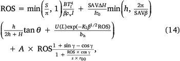


In Eqns 14–19, S is the leaf area per square metre, B is the Stefan–Boltzman constant, Tf is the absolute flame temperature, β is the fuel packing ratio, ρv is the fuel particle density, I is the ignition energy, SAV is the surface area-to-volume ratio of fine fuels, h is the height of the flame base, H is the flame height, bn is the vertical gas velocity on flat terrain, Ta is the absolute ambient temperature, g is gravity, ΔH is the heat of combustion of pyrolysis gases,  is the flame radiative fraction, cp is the specific heat of air, Q̇0 is the heat release, σ is the total fuel load, γ is the flame tilt angle, θ is the local terrain slope angle, U(L) is the midflame-height horizontal velocity calculated by QES-Winds, b is the vertical velocity inside the flame, and A is the flame radiation coefficient. The model includes three universal parameters: a flame drag coefficient K1, the stoichiometric coefficient for combustion st, and a parameter to account for flame thickness vs radiative fraction in the flame radiation model r00. Heat transfer from the flames to the fuels is attenuated through the flame length in the Balbi model; this is preserved in the formulation by QES-Fire through the parameters in the Balbi model governing the convective and radiative heat transfer, K1 and r00.
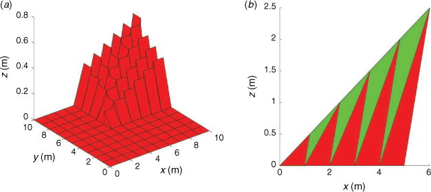
The flame tilt angle for the Balbi model returns tilt normal to the fire front. For our 3-D implementation, flame tilt is calculated separately for the x and y directions for each 2-D mapper cell. The tilt angle along the direction with the strongest horizontal wind component (e.g. U(L) in Eqn 19) is then chosen as the dominant direction and the flame over that cell is modelled as a triangular prism (Fig. 3). Calculating the tilt angle and flame geometry at each fully burning mapper cell in this manner enables a discrete approximation of flame structures that can represent individual point fires, complete fire fronts and fires burning in non-homogeneous terrain. While the prisms are modelled with the dominant wind direction, the ROS forcing for the level set method is calculated using the wind vector multiplied by the cosine of the angle between the wind and the normal to the fire front, thus preserving the formulation for ROS in the Balbi model.
|
To account for heterogeneous terrain, fuels, and winds, the flame geometry must be adapted to the QES-Winds scale ( (1 m)) from the fire front scale (
 (10 m)) assumed in the original model (Balbi et al. 2009). Using the assumption that within a flame vertical motion is uniformly accelerated owing to buoyancy and that flame outlines are streamlines (Chatelon et al. 2017), the horizontal velocity into the flame is approximately equal to the horizontal velocity out of the flame as the flame base length approaches zero. Additionally, assuming the flame residence time (τ) is inversely proportional to the surface area-to-volume ratio (τ = τ0/SAV, where τ0 is the residence time parameter; Anderson 1969), the discrete flame height can be decreased for a given Δx, where Δx = the flame base length for our discrete representation, linearly as a function of the time on fire (t) as

where H is the modified flame height and H0 is the original flame height. Thus, the Balbi geometry is recovered in 2-D using discrete prisms (Fig. 3).
Coupling the residence time dependence to the flame height with triangular prisms allows the construction of a fully 3-D fire front by aggregating the individual discrete flame models into a single fire front (Fig. 3). The ability of QES-Fire to represent surface conditions and fire front segments in a discrete manner enables heterogeneous fire fronts with varying fuel types, moisture contents and slope conditions to be modelled.
QES-Fire plume parameterisation
A major goal in the development of QES-Fire is to couple the ROS and local winds in the fire front vicinity, which enables future integration of QES-Fire with other fire-related phenomena (e.g. smoke dispersion, firebrand production and transport). This is accomplished using the axisymmetric plume model proposed by Baum and McCaffrey (1989) superimposed on the background QES-Winds velocity field. QES-Fire’s cellular nature utilises merging plumes to account for adjacent and/or dispersed heat sources.
Velocity field from axisymmetric plume
The Baum and McCaffrey (1989) model for the flow field induced by fires provides a time-averaged quasi-steady-state velocity field for an axisymmetric plume that is scaled by the surface heat flux.
McCaffrey (1983) proposed a plume model based on the conservation of mass,

conservation of momentum,

and conservation of energy equations,

where ρ is the density of air,  is the perturbation from the hydrostatic pressure, and
  is the rate of energy release from a heat source per unit volume. For a large semi-infinite plume, the length scale for non-dimensionalisation is not readily apparent. By defining generic non-dimensional variables:

substituting them into Eqns 21–23, and then performing a scale analysis, it is possible to deduce the characteristic length

and characteristic velocity

scales for an axisymmetric plume, where  is the total, volume-integrated power output of the distinct fire (Trelles 1995).
Inside the plume, the McCaffrey (1983) model assumes a non-dimensionalised Gaussian profile for both temperature,

and vertical velocity,

where  is an empirically derived non-dimensionalised centreline temperature,
  is the empirically derived non-dimensional vertical velocity scaled by the characteristic velocity wc (Eqn 26) (Baum and McCaffrey 1989), ƞ = 0.866 is the empirically determined ratio of the thermal to momentum radii of the plume (Baum and McCaffrey 1989), R* = R/Lc is the empirically fitted non-dimensionalised plume radius, r* = r/Lc is the non-dimensional radial distance from the plume centreline, and ζ* = z/Lc is the non-dimensional vertical distance from the plume source. For a single axisymmetric plume, the origin is at ground level; however, this value is adjusted to a virtual origin for merged plumes (see ‘Merging plumes’ section below).
To calculate the external flow field due to the plume, Baum and McCaffrey decompose the velocity field into potential and solenoidal flow components. Physically, the potential flow is due to the volumetric expansion of hot combustion gases while the solenoidal flow accounts for the flow induced by vorticity. Using the characteristic length and velocity, the centre-line potential can be expressed as

the centre-line vorticity as

and a centre-line pseudo streamfunction as

In cylindrical coordinates with the assumptions of an axisymmetric plume and a Gaussian distribution for the temperature (Eqn 27) and vertical velocity (Eqn 28), the non-dimensional radial ( ) and vertical (
 ) velocities can be determined from


subject to the boundary conditions for Ʌ* given by

that enforce that flow cannot cross the centreline axis (r* = 0) or the ground (ζ* = 0). For the far field potential, the expansion velocity is governed by the asymptotic value Ʌ*asymptote. This is Green’s function for potential due to a point source,

evaluated at r* = 30 and ζ* = 60. The values of r* and ζ* for the asymptotic solution correspond to a smooth transition from Eqns 32, 33 to the solution of Eqn 35. The streamfunction component of Eqns 32, 33 is calculated using the definition of vorticity,

where  is found by taking the curl of the empirically derived vertical velocity (Eqn 28),

The boundary conditions for  are
are

enforcing the fact that the plume centreline and ground form streamlines that mass may not cross. The form of  is fairly complex and described fully in Baum and McCaffrey (1989) and Trelles (1995).
The non-dimensional velocity field due to a single fire is computed as a superposition of the radial (Eqn 32) and vertical flow (Eqn 33). The result of this superposition is then scaled by the surface heat flux (Eqn 26) provided by the Balbi model (Eqn 18) for a fully burning cell, or scaled by the percentage area for a partially burning cell. This is subsequently used as a parameterisation in QES-Winds (i.e. the  ,
,  , and
, and  fields) to calculate the final total velocity field as described in the ‘Microscale winds’ section above. For multiple distinct fires, Trelles (1995) shows that the velocity fields for individual fires can be superimposed. In QES-Fire, the superposition of multiple unconnected plumes is performed prior to the final mass conservation step (see ‘Microscale winds’). When multiple distinct fires are spatially close, Trelles (1995) observed that the velocities may only be superimposed up to a height at which the plumes width begin to overlap. Above this height, the superimposed vertical velocities will overestimate the vertical velocity. Trelles (1995) gives an overview of how this may be accomplished at the asymptotic extent of the plumes; however, a new methodology is needed for merging plumes below the far field behaviour. QES-Fire’s methodology for this is described in the next section.
Merging plumes
Many studies have examined the dependence of plume merging on source buoyancy and momentum fluxes (e.g. Gebhart and Pera 1971; Davidson and Slawson 1982; Davidson 1989; Macdonald et al. 2002). Kaye and Linden (2004) is the first detailed one focused on merging turbulent axisymmetric plumes. Of particular interest for QES-Fire is the development of a criterion for when turbulent plumes merge. Prior models use the methodology that when two plumes have grown laterally enough to overlap, the height where the overlap occurs is defined as the merging height (e.g. Bjørn and Nielsen 1995). This simplistic view does not take into account mutual entrainment (Kaye and Linden 2004). Finney and McAllister (2011) show that mutual entrainment from spot fires intensifies the burning and heat release rates of fires, and therefore should be included.
QES-Fire includes the impact of mutual plume entrainment using the assumption that in the absence of mean wind, individual plumes are passively advected owing to the entrainment field of other plumes in the domain, and that for equal-strength plumes, plumes will be deflected towards each other equally (Kaye and Linden 2004). In the QES-Fire formulation, the plume-merging height is calculated based on a non-dimensional mixing height μm defined by

where x0 is the separation distance between plume sources. μm is then calculated using

where ϵ = 0.09 is an entrainment constant and  is the upper bound for the height when two non-interacting Gaussian plumes merge together (Kaye and Linden 2004). After the merging height is calculated, a new virtual origin for the merged plume is determined by (Kaye and Linden 2004)

where ζv is the distance below the merged plume sources.
For the case of unequal plumes, Eqn 40 can be modified to include the effects of the relative strengths of the plume sources as

where ĸ ≤ 1 is the ratio of the plume buoyancy fluxes. For ĸ = 1, Eqn 42 reduces to Eqn 40. μm has minimal variation for a wide range of ĸ values, approximately 25% for 0.15 ≤ ĸ ≤ 1 (Kaye and Linden 2004) and, therefore, QES-fire assumes the equal plume strength value for μm for all plume merging. This is justified based on the small grid spacing typically used in QES-Fire, which limits the variation in heat release per grid cell (Eqn 18) to approximately 30% using Anderson’s (1982) fuel model.
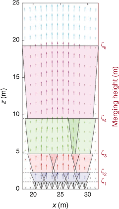
The discrete nature of the fire map (see ‘Fire map’ section above) means that nearly all simulations will require the merging of more than two plumes. This is accomplished through a multiscale aggregation operation applied to the surface heat fluxes and subsequently through the plume parameterisation (see ‘Velocity field from axisymmetric plume’) to the plume velocities. The goal is to merge adjacent plumes at the appropriate vertical position. This height is calculated by modifying Eqn 39 to yield

where x0 = Δx for the fire map and Γ is the filter index making the product Γ*x0 the plume separation distance for filter level Γ. For the ground level to the first mixing height, Γ = 1 and each grid cell in the fire map is considered a distinct plume source. The velocity field from each grid cell is then calculated and superimposed following the ‘Velocity field from axisymmetric plume’ section starting at the ground level and up to the mixing-height level ζ1. The filter is then enlarged to merge two adjacent plume sources whose separation distance is Γ*x0 = 2Δx. The next merging height ζ2 and new virtual origin ζv,2 are then computed and the velocity field from the two merged plumes is then calculated as a single source. The new source is scaled by the total heat release of the merged plumes found by summing adjacent fire map cells. The velocity field is then superimposed for each merged plume in the vertical from ζ1 to ζ2. This continues until the top of QES-Fire’s domain is reached or until all plumes are merged into a single source. A schematic view of this plume-merging process is given in Fig. 4.
|
The plume-merging methodology serves two critical purposes in QES-Fire. First, it allows for the superposition of distinct plumes parameterised with the axisymmetric plume model described in the ‘Velocity field from axisymmetric plume’ section in a physically realistic manner and second, it gives QES-Fire the ability to have a cell-based fire map that is computationally efficient. The total merged plume from a fire front made of several sources is shown in Fig. 5.
QES-Fire comparison
Examination of QES-Fire’s performance is accomplished in two phases. First, the plume structure parameterisations (independent of the ROS) are compared with high-resolution unsteady plume resolving large-eddy simulations (LESs) using WRF-SFIRE (Mandel et al. 2011, 2014). Next, the FireFlux II field campaign (Clements et al. 2019) is used to validate QES-Fire’s ROS and compare its calculated wind velocities with in situ velocity measurements taken during an experimental burn.
Idealised plume validation
High-resolution LES runs of WRF-SFIRE were performed to examine the quality of QES-Fire’s plume parameterisations. Two WRF-SFIRE simulations were performed, a ‘large’ burn area case and a ‘small’ burn area case. Both simulations used a 3 km × 3 km × 3 km atmospheric domain discretised with 120 × 120 × 120 grid points, resulting in a uniform grid spacing of Δx = Δy = Δz = 25 m. The burn area was modelled using the SFIRE land surface module run on a grid one fifth the size of the atmospheric grid with a grid spacing of Δx = Δy = Δz = 5 m. The small burn area was a 25 m × 25 m square and the large burn area was 50m × 50 m, both with constant heat fluxes of 72.14 kW m−2. The heat fluxes were injected into the atmospheric model over an extinction depth (Mandel et al. 2011). For the small burn area, the depth was specified as 40 m, and for the large burn area, the depth was specified as 55 m. The extinction depth was chosen based on the McCaffrey (1983) temperature profile for a flame with a comparable heat flux. The simulations were run for 20 min each with zero ambient winds and neutral background stratification. Prognostic variables were output every 20 s. After a 15-min spin-up, output data from the final 5 min of the WRF-SFIRE simulations were time-averaged to calculate plume statistics for comparison with QES-Fire’s steady-state fields. Tests with different spin-up times and grid resolutions resulted in negligible differences in presented statistics. The computation time for each of the WRF-SFIRE simulations was 3300 s on 32 Intel XeonSP Skylake cores. QES-Fire was run for the same two test cases with the same grid resolution (Δx = Δy = Δz = 25 m) and took 12 s on a single Intel XeonSP Skylake core with an NVIDIA® Titan V GPU.
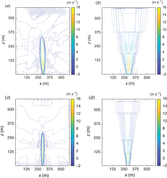
Fig. 6 depicts the time-averaged vertical velocity through the axisymmetric plume centre for both WRF-SFIRE and QES-Fire. Near the ground, QES-Fire has a broader area of strong upward vertical velocity compared with WRF-SFIRE. This is due to QES-Fire’s use of individual plumes at each surface grid cell, all of which contribute to the near-ground vertical velocity. The wider plume base in QES-Fire results in a wider plume at all vertical levels and translates into a shorter core-region of high vertical velocity (e.g. velocities greater than 5 m s−1).
|
Although the core region of high vertical velocity is shorter, QES-Fire’s plume extends to a higher level in the vertical direction when all positive vertical velocity values are considered. QES-Fire does not account for atmospheric stability. As a result, the buoyant plume in QES-Fire is only weakly confined in the vertical direction. LES models such as WRF-SFIRE that solve the momentum and energy equations limit the extent of vertical transport through the temperature field. The only limitation on the vertical extent of the plume rise in QES-Fire is from the Baum and McCaffrey (1989) plume model, particularly the asymptotic behaviour of the model at ζ* = 60 (ζ = 460 m for the large and ζ = 262 m for the small heat flux plots).
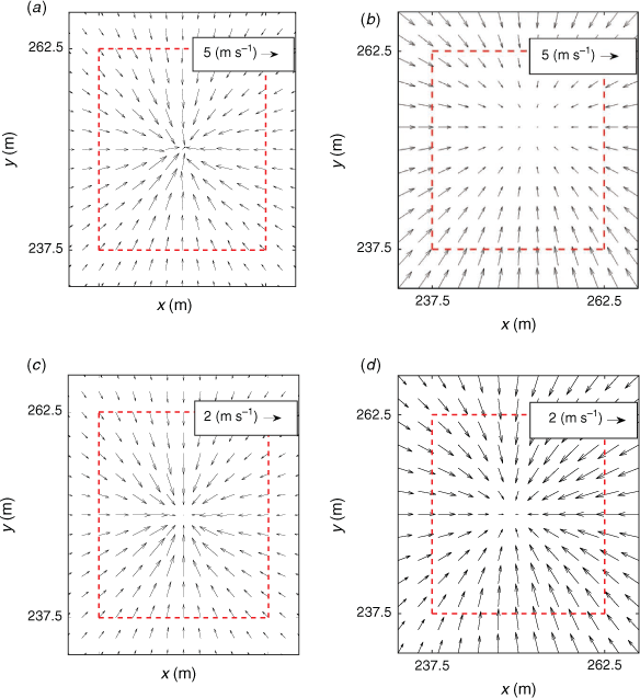
In addition to the structure of the vertical plume winds, it is of interest to understand the performance of QES-Fire’s horizontal winds compared with WRF-SFIRE’s owing to their key role in coupling the fire front–atmospheric winds to the ROS model in QES-Fire. The horizontal winds were examined at heights for which the Baum and McCaffrey (1989) model predicts the equivalent for a mid-flame region for the calculated heat flux: 10 m for the large burn area and 7 m for the small burn area (Fig. 7). Vectors in the figure have nearly identical patterns and a similar entrainment velocity at the heat flux perimeter for both models. For the large burn area, the average horizontal velocity across the heat flux perimeter for the WRF-SFIRE idealised plume is 4.75 m s−1, vs 5.34 m s−1 for QES-Fire. For the small burn area, the average horizontal velocity across the heat flux perimeter for the WRF-SFIRE idealised plume is 1.92 m s−1 vs 2.11 m s−1 for QES-Fire.
|
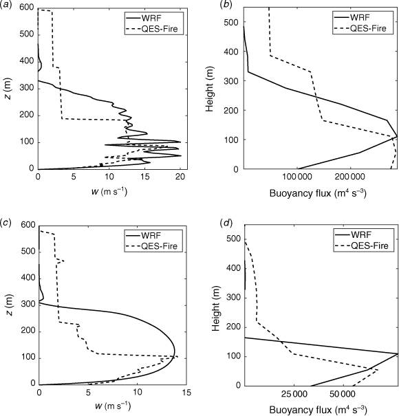
A clear difference between QES-Fire and WRF-SFIRE plumes is the vertical and horizontal extent of the plumes they create. Still, the centreline vertical velocity values of the two models agree well near the ground (Fig. 8). The magnitudes of the centreline vertical velocities agree but the profile shapes have two clear differences. The first is the distinct steps in the QES-Fire profile. These steps correspond to the plume mixing height levels and are a direct result of the merging plumes modelling methodology (see ‘Merging plumes’ above). The second difference is also evident from the vertical velocity contour plots (Fig. 6). The QES-Fire centreline vertical velocity decreases significantly at a lower vertical level than in WRF-SFIRE (200 m vs 250 m for the large burn area, and 110 m vs 250 m for the small burn area) but then continues with a small value to a much greater height.
|
A direct result of QES-Fire’s broader plume but similar vertical velocity values is an increase in the integrated buoyancy flux compared with WRF-SFIRE at the surface (Fig. 8). However, as we move away from the ground, the total buoyancy fluxes through the x−y plane at a given height are comparable between the two models. Overall, the domain-integrated buoyancy flux for the plume from the large burn area is 1.36 × 10⁶ m4 s−3 in WRF-SFIRE whereas in QES-Fire it is 1.61 × 10⁶ m4 s−3, a relative difference of less than 15%. For the small burn area, the domain integrated buoyancy flux is 1.58 × 10⁵ m4 s−3 in WRF-SFIRE whereas in QES-Fire it is 1.89 × 10⁵ m4 s−3, a relative difference of less than 17%.
To examine the grid resolution dependence of the QES plume-merging methodology, the large burn area was simulated with QES-Fire for a range of grid cell sizes. For a cell the size of the burn area, there is no merging and the Baum and McCaffrey (1989) plume model (see ‘Velocity field from axisymmetric plume’) holds exactly. As the burn area is broken into multiple QES cells, the plumes should merge in the vertical direction to create a single plume with a maximum velocity that is the same as the single plume case. For a 50 m × 50 m burn area, the maximum vertical velocity from a single plume was calculated as 19.53 m s−1. The maximum velocities for Δx = Δy = 2–50 m varied between 19.53 and 20.72 m s−1, a maximum relative difference of 7%, demonstrating QES-Fire’s ability to represent the vertical velocity structure for a single plume using its discrete surface representation (see ‘Merging plumes’).
Experimental burn validation
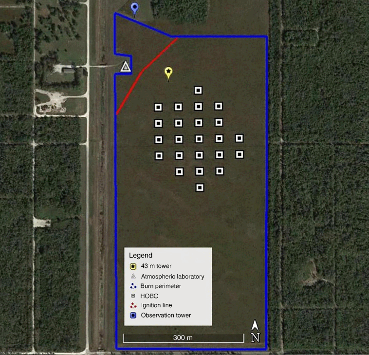
The FireFlux II (FFII) experiment provides a valuable dataset of in situ measurements during a prescribed burn. FFII was conducted in a Texas grass plot over flat land where topography plays a minimal role in the fire spread. The site is described in detail in Clements et al. (2007), and the experimental setup for FFII in Clements et al. (2019) (see Fig. 9 for a schematic). Here, we briefly review the most salient measurements used to validate QES-Fire.
|
The ROS calculations for the field data are made from an array of 24 HOBO® temperature loggers recording at 1 Hz. Each HOBO logger was equipped with an Omega 20-gauge K-type thermocouple to measure the temperature just above the soil. The HOBO loggers were arranged in a grid with 50-m spacing in the burn plot to track the fire front progression. The arrival time of the fire front was taken to be when the temperature first exceeded 400°C.
Ambient wind forcing data required to run QES-Fire are provided by the University of Houston Atmospheric Laboratory (HAL) tower located on the western edge of the burn plot. Additionally, a 43-m micrometeorology tower located in the burn plot fitted with 3-D sonic anemometers and type T thermocouples at heights of 5.8-m, 10-m and 20-m provides wind and temperature data for validation purposes. A planar fit tilt correction was applied to the sonic anemometer velocity components (Wilczak et al. 2001) using the 24-h period prior to the experimental burn. Wind forcing for QES-Fire was specified using the average windspeed (10 m s−1) and direction (310°) over the 30-min time period prior to the start of the experiment taken from the HAL tower sonic anemometer at a height of 31 m. Winds were then interpolated using a log-law profile with an aerodynamic roughness length (l0) of 0.15 m corresponding to a field of uncut tall grass (Stull 2003). The horizontal turbulence strength from the HAL tower was calculated as the root mean square of the turbulent fluctuations (2.09 m s−1) beginning 30 min prior to ignition through the end of the burn. The turbulence intensity was then determined to be 0.21, justifying the use of a quasi-steady-state model with a single wind forcing.
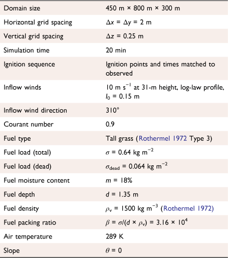
Fuels were sampled throughout the burn plot 30 min prior to the burn. Based on this sampling, the appropriate fuel type was determined to be tall grass. The fuel load was specified as 0.64 kg m−2 with a moisture content of 18% (Clements et al. 2019). The Balbi model requires the fuel load for both live and dead fuels. Because the composition of live vs dead fuel load was unknown for the FFII burn, a conservative estimate that the dead fuel load accounted for 10% of the total fuel load was specified. Sensitivity testing found a 3% relative error in the ROS for a 25% change in dead fuel load vs total fuel load. The ambient temperature taken via a radiosonde sounding just before ignition was 16°C. The ignition line for FFII was tracked and timed based on video taken from a GoPro® camera mounted at 40-m on an observation tower in the northwest corner of the burn plot. This ignition sequence was read into QES-Fire, and at the specified times and locations in the burn plot, a new ignition was created to accurately describe the ignition procedure. Once the fire front is initiated and the background winds are specified, QES-Fire is used to propagate the fire front following the procedure detailed in ‘QES-Fire modelling methodology’ above (see Table 2 for a summary of input parameters).
|
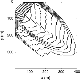
One of the most critical aspects to evaluate for any wildfire spread model is its ability to create realistic fire fronts that move at realistic ROSs. QES-Fire’s calculated fire front progression for the FFII controlled burn is shown in Fig. 10. Based on qualitative comparisons with video taken from the observation tower GoPro camera, QES-Fire captures the general shape and progression pattern (i.e. isochrones) of the experiment. It is noteworthy that while the forward progression of the fire front matches field data quite well, the backing fire front ROS is overestimated. This is likely a result of the model’s induced winds because the ROS model predicts negligible forcing for the level set when winds are opposed to the fire front.
|
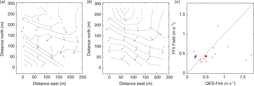
A more quantitative examination of the ability of QES-Fire to accurately represent the FFII fire front progression can be preformed by comparing the QES-Fire ROS with the ROS calculated from the HOBO data loggers. This is facilitated by QES-Fire’s calculation of the ROS vector at each grid cell that is on fire (see ‘Fire map’ section) at each model time step, allowing for a direct comparison at points matching the HOBO data (Fig. 11). Additionally, isochrones from the QES-Fire fire front and the experimental data fire front have been calculated to enable direct comparisons of the fire front shape as it progresses through the HOBO array.
The isochrones calculated by QES-Fire have the same general shape as those calculated for FFII. The primary differences in the ROS and isochrones between the model and the experiment occurs at two HOBO points in a region near 50–125 m east and 75–150 m north where QES-Fire predicts a rapid acceleration of the fire front that is not observed in the data. Comparison of the ROS from FFII and QES-Fire through the HOBO array shows a root mean squared error (RMSE) of 0.22 m s−1 with a mean ROS of 0.53 m s−1 for QES-Fire compared with 0.43 m s−1 from the field data. There is an overestimation of the ROS for the western flank of the fire front. This is most likely a result of the acceleration of the fire front due to the level set combined with the fact that QES-Fire does not account for changes in ambient winds present during the experiment. On the leading edge of the fire front, there is a slight underestimation of the ROS, 0.92 m s−1 for QES-Fire vs 0.95 m s−1 observed in the experiment. If the Balbi model is used without flame mid-height surface wind feedback from QES-Fire, the average ROS drops below the experimental data to a value of 0.32 m s−1.
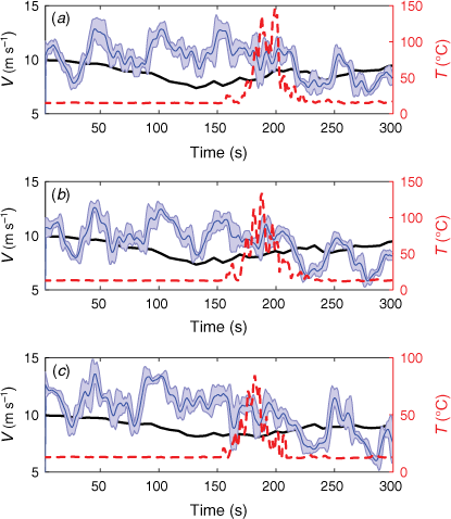
Of particular interest is the accuracy of QES-Fire’s horizontal wind predictions in the vicinity of the fire front. These winds drive the ROS and serve as one of the primary coupling mechanisms between the fire front and the atmospheric flow. To validate QES-Fire’s fire-induced winds, comparisons are made with the anemometers on the 43-m tower in the FFII burn plot (Fig. 12). Because QES-Fire is a quasi-steady-state model that represents the ensemble mean value of the velocity vector and to facilitate visual comparisons, the QES-Fire horizontal winds are examined relative to the experimental horizontal winds averaged with a 3-s moving average, corresponding to the fire front residence time. The most notable feature in the horizontal winds is a decrease as the fire front approaches the 43-m tower. The decrease is linked to the fire-induced winds causing entrainment into the flame plume. Once the fire front passes the tower, there is an increase in the velocity as the fire-induced winds add to the ambient winds. The effect is most prominently exhibited at the 6-m measurement height but persists up to the 20-m level. Both QES-Fire and the field data exhibit this behaviour, with the trend more pronounced in QES-Fire. QES-Fire’s behaviour is a result of the fire line and plume parameterisation models. Additionally, the aerodynamic roughness length (l0) is decreased as the fuel is consumed by the fire front. This decrease in l0 corresponds to an increase in the near-surface horizontal winds calculated by QES-Winds supporting the conclusion of Sun et al. (2009) that a decrease in l0 may have a significant impact on ROS. Overall, the general ability of QES-Fire to predict horizontal winds is considered to be acceptable. RMSEs of horizontal velocity for QES-Fire vs field data are 1.48 m s−1 at the 6-m height measurement position, 1.90 m s−1 at the 10-m height, and 0.69 m s−1 at the 20-m height.
|
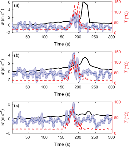
To examine how well QES-Fire captures key features of the vertical velocity near the fire line, it is compared against the sonic anemometer data smoothed with a 3-s moving average from the 43-m tower (Fig. 13).
|
The clearest signature in the vertical velocity time series is an increase in upward magnitude. The increase is evident in the field data and the QES-Fire modelled winds. Away from the ground, at the 10-m and 20-m heights, the magnitude of QES-Fire’s peak vertical velocity agrees reasonably well with the values in the field data. Near the ground at the 6-m measurement height, QES-Fire clearly overestimates the upward vertical velocity. The increased overestimation near the ground is consistent with our examination of QES-Fire’s plume-merging parameterisation (see ‘Merging plumes’ above) where the distributed nature of the model near the ground results in enhanced vertical velocity. During the experimental burn, a large-scale subsidence of approximately −0.5 m s−1 was observed, leading to a mean negative value in the vertical velocity prior to, and after, the fire front passage at the 43-m tower. Because the subsidence is presumably not local to the burn plot and not explicitly included in the QES-Fire forcing, it is not captured by QES-Fire and explains some of the discrepancy in the comparison of vertical velocities. The arrival time of the peak vertical velocity in the QES-Fire predictions is also observed to lag the field observation’s arrival at all heights. The delay agrees with the slightly delayed fire line progression (Fig. 11) through the HOBO array. To a lesser extent, a second likely explanation for the delayed timing is the lack of direct inclusion of cross-wind advection in the QES-Fire plume parameterisation. The FFII burn occurred under strong winds, which tilt the plume in the downwind direction resulting in earlier plume arrival times for measurement points that are higher off the ground. Although not strong, this phenomenon can be observed in the tower wind and temperature fields (Figs 12, 13). In addition to altering the plume arrival time, the lack of a specific cross-wind parameterisation in QES-Fire likely contributes to the overestimation of the maximum vertical winds in the plume, especially for the higher measurement heights. While not as good as the horizontal velocity predictions, the vertical velocity predicted by QES-Fire is also acceptable considering the complexity of the simulated process. Vertical velocity RMSEs for QES-Fire vs field data are 1.15 m s−1 at the 6-m height measurement position, 1.00 m s−1 at the 10-m height, and 1.22 m s−1 at the 20-m height.
Summary
This work presents a fast-response microscale wildfire progression model, QES-Fire. It incorporates three simplified physics quasi-steady-state models: a diagnostic wind solver (QES-Winds), a surface fire ROS model (the Balbi model), and a buoyant plume rise model that includes merging plumes. QES-Fire dynamically couples the background wind velocities to the fire-induced winds through the plume rise model and wind solver, and incorporates this new velocity field as a direct driver to the ROS model, providing high-resolution inputs for calculation of ROS and a highly realistic wind field in the vicinity of the fire front.
QES-Fire’s fire-induced winds are compared against high-resolution LES of idealised buoyant plumes, yielding results with relative errors for the maximum centreline vertical velocity of 10% for a large burn area and 6% for a small burn area at a fraction of the computational cost. In addition, the buoyant fluxes have a relative error of 15% for the large burn plot and 17% for the small burn plot. To challenge QES-Fire to a more realistic scenario, ROS and wind velocities, both vertical and horizontal, are compared against the FireFlux II field experiment data and are in good agreement with observed results for flat terrain with homogeneous fuel. Backing fire front ROS is overestimated and requires further investigation.
Additional model development for QES-Fire is needed to extend its use to more general cases. This includes the effects of terrain on the coupled feedback with the winds, both the effects the terrain has on the local winds and the impact of terrain on the plume parameterisations. The general impact of ambient winds on the fire plume should also be explored, especially how coupling with terrain-induced winds can lead to extreme fire behaviours (Sharples et al. 2012). The overall goal of QES-Fire is to provide rapid fire evolution forecasts that account for fire–atmosphere coupling at the microscale. These forecasts could be used to support fire operations and prescribed burns or used as a research tool to explore coupling processes. QES-Fire’s faster-than-real-time calculations using quite modest computational resources allows examination of how changes in variables (e.g. wind speed, wind direction, fuel moisture) affect the ROS. Ensemble runs of QES-Fire can help in assessing the risk fire fronts pose due to changes in coupled fire–atmospheric conditions.
Future work will also take advantage of other aspects of the QES framework including its Lagrangian particle dispersion model (Singh et al. 2011), which may be used for firebrand and smoke transport. In addition, QES-Winds was primarily developed for and validated in urban environments with resolved buildings (Bozorgmehr et al. 2021). Hence QES-Fire is well positioned to be adapted for fires at the wildland–urban interface.
Data availability
Data sharing is not applicable as no new data were generated or analysed during this study.
Conflicts of interest
The authors declare no conflicts of interest.
Declaration of funding
This research was supported by the National Science Foundation under grant PREEVENTS 1664175, the University of California Office of the President award LFR-20-651032, USDA NIFA Hatch project no. 1013396, NASA grant 80NSSC19K1091, and NSF grants DEB-2039552.
References
Achtemeier GL (2013) Field validation of a free-agent cellular automata model of fire spread with fire–atmosphere coupling. International Journal of Wildland Fire 22, 148–156.| Field validation of a free-agent cellular automata model of fire spread with fire–atmosphere coupling.Crossref | GoogleScholarGoogle Scholar |
Albini FA (1979) Spot fire distance from burning trees - a predictive model. Technical Report INT-56, USDA Forests Service, Intermountain Forest and Range Experiment Station. (Ogden, UT)
Albini FA (1982) Response of free-burning fires to nonsteady wind. Combustion Science and Technology 29, 225–241.
| Response of free-burning fires to nonsteady wind.Crossref | GoogleScholarGoogle Scholar |
Anderson HA (1969) Heat transfer and fire spread. Technical Report INT-69, USDA Forests Service, Intermountain Forest and Range Experiment Station. (Ogden, UT)
Anderson HA (1982) Aids to determining fuel models for estimating fire behavior. Technical Report INT-122, USDA Forests Service, Intermountain Forest and Range Experiment Station. (Ogden, UT)
Baker BB, Copson ET (2003) ‘The mathematical theory of Huygens’ principle. Vol. 329.’, (American Mathematical Society (Chelsea Publishing, Providence))
Balbi JH, Morandini F, Silvani X, Filippi JB, Rinieri F (2009) A physical model for wildland fires. Combustion and Flame 156, 2217–2230.
| A physical model for wildland fires.Crossref | GoogleScholarGoogle Scholar |
Balbi JH, Rossi JL, Marcelli T, Chatelon FJ (2010) Physical modeling of surface fire under nonparallel wind and slope conditions. Combustion Science and Technology 182, 922–939.
| Physical modeling of surface fire under nonparallel wind and slope conditions.Crossref | GoogleScholarGoogle Scholar |
Balbi JH, Chatelon FJ, Morvan D, Rossi JL, Marcelli T, Morandini A (2020) A convective–radiative propagation model for wildland fires. International Journal of Wildland Fire 29, 723–738.
| A convective–radiative propagation model for wildland fires.Crossref | GoogleScholarGoogle Scholar |
Barbano F, DiSabatino S, Stoll R, Pardyjak ER (2020) A numerical study of the impact of vegetation on mean and turbulence fields in a european-city neighbourhood. Building and Environment 186, 107293
| A numerical study of the impact of vegetation on mean and turbulence fields in a european-city neighbourhood.Crossref | GoogleScholarGoogle Scholar |
Baum HR, McCaffrey BJ (1989) Fire induced flow field - theory and experiment. Fire Safety Science 2, 129–148.
| Fire induced flow field - theory and experiment.Crossref | GoogleScholarGoogle Scholar |
BC Wildfire Services (2020) Wildfires of note. Available at http://bcfireinfo.for.gov.bc.ca/hprScripts/WildfireNews/OneFire.asp [Verified 6 September 2020]
Bjørn E, Nielsen PV (1995) ‘Merging thermal plumes in the indoor environment.’ (Department of Building Technology and Structural Engineering, Aalborg University)
Bozorgmehr B, Willemsen P, Gibbs JA, Stoll R, Kim JJ, Pardyjak ER (2021) Utilizing dynamic parallelism in CUDA to accelerate a 3D red-black successive over relaxation wind-field solver. Environmental Modelling & Software 137, 104958
| Utilizing dynamic parallelism in CUDA to accelerate a 3D red-black successive over relaxation wind-field solver.Crossref | GoogleScholarGoogle Scholar |
Brown MJ, Gowardhan AA, Nelson MA, Williams MD, Pardyjak ER (2013) QUIC transport and dispersion modelling of two releases from the joint urban 2003 field experiment. International Journal of Environment and Pollution 52, 263–287.
| QUIC transport and dispersion modelling of two releases from the joint urban 2003 field experiment.Crossref | GoogleScholarGoogle Scholar |
Chatelon FJ, Balbi JH, Morvan D, Rossi JH, Marcelli T (2017) A convective model for laboratory fires with well-ordered vertically-oriented fuel beds. Fire Safety Journal 90, 54–61.
| A convective model for laboratory fires with well-ordered vertically-oriented fuel beds.Crossref | GoogleScholarGoogle Scholar |
Clark TL, Coen J, Latham D (2004) Description of a coupled atmosphere–fire model. International Journal of Wildland Fire 13, 49–63.
| Description of a coupled atmosphere–fire model.Crossref | GoogleScholarGoogle Scholar |
Clements CB, Zhong S, Goodrick S, Li J, Potter BE, Bian X, Heilman WE, Charney JJ, Perna R, Jang M, et al. (2007) Observing the dynamics of wildland grass fires: Fireflux - a field validation experiment. Bulletin of the American Meteorological Society 88, 1369–1382.
Clements CB, Kochanski AK, Seto D, Davis B, Camacho C, Lareau NP, Contezac J, Restaino J, Heilman WE, Krueger SK, Butler B (2019) The FireFlux II experiment: a model-guided field experiment to improve understanding of fire–atmosphere interactions and fire spread. International Journal of Wildland Fire 28, 308–326.
| The FireFlux II experiment: a model-guided field experiment to improve understanding of fire–atmosphere interactions and fire spread.Crossref | GoogleScholarGoogle Scholar |
Coen J (2013) Modeling wildland fires: A description of the Coupled Atmosphere–Wildland Fire Environment model (CAWFE) (No. NCAR/TN-500+STR). National Center for Atmospheric Research, Boulder, CO.
| Crossref |
Coen JL, Cameron M, Michalakes J, Patton EG, Riggan PJ, Yedinak KM (2013) WRF-Fire: coupled weather–wildland fire modeling with the weather research and forecasting model. Journal of Applied Meteorology and Climatology 52, 16–38.
| WRF-Fire: coupled weather–wildland fire modeling with the weather research and forecasting model.Crossref | GoogleScholarGoogle Scholar |
Davidson GA (1989) Simultaneous trajectory and dilution predictions from a simple integral plume model. Atmospheric Environment 23, 341–349.
| Simultaneous trajectory and dilution predictions from a simple integral plume model.Crossref | GoogleScholarGoogle Scholar |
Davidson GA, Slawson PR (1982) Effective source flux parameters for use in analytical plume rise models. Atmospheric Environment 16, 223–227.
| Effective source flux parameters for use in analytical plume rise models.Crossref | GoogleScholarGoogle Scholar |
Deeming JE (1977) The national fire-danger rating system, 1978. Technical report, USDA Forest Service, Intermountain Forest and Range Experiment Station. (Ogden, UT)
Ferziger JH, Peric M (2002) ‘Computational Methods for Fluid Dynamics.’ (Springer Publishing: New York, NY)
Filippi JB, Bosseur F, Pialat X, Santoni PA, Strada S, Mari C (2011) Simulation of coupled fire/atmosphere interaction with the MesoNH-ForeFire models. Journal of Combustion
| Simulation of coupled fire/atmosphere interaction with the MesoNH-ForeFire models.Crossref | GoogleScholarGoogle Scholar |
Filippi JB, Pialat X, Clements CB (2013) Assessment of ForeFire/Meso-NH for wildland fire/atmosphere coupled simulation of the FireFlux experiment. Proceedings of the Combustion Institute 34.2, 2633–2640.
| Assessment of ForeFire/Meso-NH for wildland fire/atmosphere coupled simulation of the FireFlux experiment.Crossref | GoogleScholarGoogle Scholar |
Finney MA, McAllister SS (2011) A review of fire interactions and mass fires. Journal of Combustion 2011, 14
| A review of fire interactions and mass fires.Crossref | GoogleScholarGoogle Scholar |
Finney MA, Weise DR, Martin RE (1995) FARSITE: A fire area simulator for fire managers. Technical Report PSW-GTR-158, USDA Forest Service, Pacific Southwest Research Station. (Portland, OR)
Gebhart B, Pera L (1971) The nature of vertical natural convection flows resulting from the combined buoyancy effects of thermal and mass diffusion. International Journal of Heat and Mass Transfer 14, 2025–2050.
| The nature of vertical natural convection flows resulting from the combined buoyancy effects of thermal and mass diffusion.Crossref | GoogleScholarGoogle Scholar |
Hayati AN, Stoll R, Kim JJ, Harman T, Nelson MA, Brown MJ, Pardyjak ER (2017) Comprehensive evaluation of fast-response, Reynolds-averaged Navier–Stokes, and large-eddy simulation methods against high-spatial-resolution wind-tunnel data in step-down street canyons. Boundary-Layer Meteorology 164, 217–247.
| Comprehensive evaluation of fast-response, Reynolds-averaged Navier–Stokes, and large-eddy simulation methods against high-spatial-resolution wind-tunnel data in step-down street canyons.Crossref | GoogleScholarGoogle Scholar |
Hayati AN, Stoll R, Pardyjak ER, Harman T, Kim JJ (2019) Comparative metrics for computational approaches in non-uniform street-canyon flows. Building and Environment 158, 16–27.
| Comparative metrics for computational approaches in non-uniform street-canyon flows.Crossref | GoogleScholarGoogle Scholar |
Kaplan H, Dinar N (1996) A lagrangian dispersion model for calculating concentration distribution within a built-up domain. Atmospheric Environment 30, 4197–4207.
| A lagrangian dispersion model for calculating concentration distribution within a built-up domain.Crossref | GoogleScholarGoogle Scholar |
Kaye NB, Linden PF (2004) Coalescing axisymmetric turbulent plumes. Journal of Fluid Mechanics 502, 41–63.
| Coalescing axisymmetric turbulent plumes.Crossref | GoogleScholarGoogle Scholar |
Kochanski AK, Jenkins MA, Mandel J, Beezley JD, Krueger SK (2013) Real time simulation of 2007 Santa Ana fires. Forest Ecology and Management 294, 136–149.
| Real time simulation of 2007 Santa Ana fires.Crossref | GoogleScholarGoogle Scholar |
Lautenberger C (2013) Wildland fire modeling with an Eulerian level set method and automated calibration. Fire Safety Journal 62, 289–298.
| Wildland fire modeling with an Eulerian level set method and automated calibration.Crossref | GoogleScholarGoogle Scholar |
Linn R, Reisner J, Colman JJ, Winterkamp J (2002) Studying wildfire behavior using FIRETEC. International Journal of Wildland Fire 11, 233–246.
| Studying wildfire behavior using FIRETEC.Crossref | GoogleScholarGoogle Scholar |
Linn RR, Goodrick SL, Brambilla S, Brown MJ, Middleton RS, O’Brien JJ, Hiers JK (2020) QUIC-fire: A fast-running simulation tool for prescribed fire planning. Environmental Modelling and Software 125, 104616
| QUIC-fire: A fast-running simulation tool for prescribed fire planning.Crossref | GoogleScholarGoogle Scholar |
Macdonald RW, Strom RK, Slawson PR (2002) Water flume study of the enhancement of buoyant rise in pairs of merging plumes. Atmospheric Environment 36, 4603–4615.
| Water flume study of the enhancement of buoyant rise in pairs of merging plumes.Crossref | GoogleScholarGoogle Scholar |
Mallet V, Keyes DE, Fendell FE (2009) Modeling wildland fire propagation with level set methods. Computers & Mathematics with Applications 57, 1089–1101.
| Modeling wildland fire propagation with level set methods.Crossref | GoogleScholarGoogle Scholar |
Mandel J, Beezley JD, Kochanski AK (2011) Coupled atmosphere-wildland fire modeling with WRF 3.3 and SFIRE 2011. Geoscientific Model Development 4, 591–610.
| Coupled atmosphere-wildland fire modeling with WRF 3.3 and SFIRE 2011.Crossref | GoogleScholarGoogle Scholar |
Mandel J, Amram S, Beezley JD, Kelman G, Kochanski AK, Kondratenko VY, Lynn BH, Regev B, Vejmelka M (2014) Recent advances and applications of WRF & SFIRE. Natural Hazards and Earth System Sciences 14, 2829–2845.
| Recent advances and applications of WRF & SFIRE.Crossref | GoogleScholarGoogle Scholar |
McCaffrey BJ (1983) Momentum implications for buoyant diffusion flames. Combustion and Flame 52, 149–167.
| Momentum implications for buoyant diffusion flames.Crossref | GoogleScholarGoogle Scholar |
Mell W, Jenkins MA, Gould J, Cheney P (2007) A physics-based approach to modelling grassland fires. International Journal of Wildland Fire 16, 1–22.
| A physics-based approach to modelling grassland fires.Crossref | GoogleScholarGoogle Scholar |
Morvan D, Dupuy JL (2004) Modeling the propagation of a wildfire through a Mediterranean shrub using a multiphase formulation. Combustion and Flame 138, 199–210.
| Modeling the propagation of a wildfire through a Mediterranean shrub using a multiphase formulation.Crossref | GoogleScholarGoogle Scholar |
Morvan D, Meradji S, Accary G (2009) Physical modelling of fire spread in grasslands. Fire Safety Journal 44, 50–61.
| Physical modelling of fire spread in grasslands.Crossref | GoogleScholarGoogle Scholar |
Muñoz-Esparza D, Kosović B, Jiménez P A, Coen JL (2018) An accurate fire-spread algorithm in the Weather Research and Forecasting model using the level-set method. Journal of Advances in Modeling Earth Systems 10, 908–926.
| An accurate fire-spread algorithm in the Weather Research and Forecasting model using the level-set method.Crossref | GoogleScholarGoogle Scholar |
National Interagency Fire Center (2020) Statistics. Available at https://www.nifc.gov/fireInfo/fireInfo\_statistics.html [Verified 22 October 2020]
Nelson Jr RM (2000) Prediction of diurnal change in 10-h fuel stick moisture content. Canadian Journal of Forest Research 30, 1071–1087.
| Prediction of diurnal change in 10-h fuel stick moisture content.Crossref | GoogleScholarGoogle Scholar |
Pagni PJ, Peterson TG (1973) Flame spread through porous fuels. Fourteenth Symposium (International) on Combustion 14, 1099–1107.
| Flame spread through porous fuels.Crossref | GoogleScholarGoogle Scholar |
Pardyjak ER, Brown MJ (2003) ‘QUIC-URB v. 1.1: Theory and user’s guide.’ (Los Alamos National Laboratory: Los Alamos, NM)
Rehm RG, McDermott RJ (2009) ‘fire front propagation using the level set method.’ (US Department of Commerce, National Institute of Standards and Technology: Gaithersburg, MD)
Röckle R (1990) Bestimmung der Strömungsverhältnisse im Bereich komplexer Bebauungsstrukturen.
Rothermel RC (1972) A mathematical model for predicting fire spread in wildland fuels. Technical Report INT-115, USDA Forest Service, Intermountain Forest and Range Experiment Station. (Ogden, UT)
Rothermel RC (1991) Predicting behavior and size of crown fires in the northern rocky mountains. Technical Report INT-RP-438, USDA Forest Service, Intermountain Forest and Range Experiment Station. (Ogden, UT)
Sethian JA (1999) ‘Level set methods and fast marching methods: evolving interfaces in computational geometry, fluid mechanics, computer vision, and materials science, volume 3.’ (Cambridge University Press: New York, NY)
Sharples JJ, McRae RHD, Wilkes SR (2012) Wind–terrain effects on the propagation of wildfires in rugged terrain: fire channelling. International Journal of Wildland Fire 21, 282–296.
| Wind–terrain effects on the propagation of wildfires in rugged terrain: fire channelling.Crossref | GoogleScholarGoogle Scholar |
Singh B, Hansen BS, Brown MJ, Pardyjak ER (2008) Evaluation of the QUIC-URB fast response urban wind model for a cubical building array and wide building street canyon. Environmental Fluid Mechanics 8, 281–312.
| Evaluation of the QUIC-URB fast response urban wind model for a cubical building array and wide building street canyon.Crossref | GoogleScholarGoogle Scholar |
Singh B, Pardyjak ER, Norgren A, Willemsen P (2011) Accelerating urban fast response lagrangian dispersion simulations using inexpensive graphics processor parallelism. Environmental Modelling & Software 26, 739–750.
| Accelerating urban fast response lagrangian dispersion simulations using inexpensive graphics processor parallelism.Crossref | GoogleScholarGoogle Scholar |
Skamarock WC, Klemp JB (2008) A time-split nonhydrostatic atmospheric model for weather research and forecasting applications. Journal of Computational Physics 227, 3465–3485.
| A time-split nonhydrostatic atmospheric model for weather research and forecasting applications.Crossref | GoogleScholarGoogle Scholar |
Stull RB (2003) ‘An Introduction to Boundary Layer Meteorology.’ (Kluwer Academic Publishers: Dordrecht)
Sullivan AL (2009a) Wildland surface fire spread modelling, 1990 - 2007. 1: Physical and quasi-physical models. International Journal of Wildland Fire 18, 349–368.
| Wildland surface fire spread modelling, 1990 - 2007. 1: Physical and quasi-physical models.Crossref | GoogleScholarGoogle Scholar |
Sullivan AL (2009b) Wildland surface fire spread modelling, 1990 - 2007. 2: Empirical and quasi-empirical models. International Journal of Wildland Fire 18, 369–386.
| Wildland surface fire spread modelling, 1990 - 2007. 2: Empirical and quasi-empirical models.Crossref | GoogleScholarGoogle Scholar |
Sullivan AL (2009c) Wildland surface fire spread modelling, 1990 - 2007. 3: Simulation and mathematical analogue models. International Journal of Wildland Fire 18, 387–403.
| Wildland surface fire spread modelling, 1990 - 2007. 3: Simulation and mathematical analogue models.Crossref | GoogleScholarGoogle Scholar |
Sun R, Krueger SK, Jenkins MA, Zulauf MA, Charney JJ (2009) The importance of fire-atmosphere coupling and boundary-layer turbulence to wildfire spread. International Journal of Wildland Fire 18, 50–60.
| The importance of fire-atmosphere coupling and boundary-layer turbulence to wildfire spread.Crossref | GoogleScholarGoogle Scholar |
Trelles JJ (1995) Mass fire modeling of the 20 October 1991 Oakland Hills Fire. PhD thesis, University of California, Berkeley.
Van Wagner CE (1977) Conditions for the start and spread of crown fire. Canadian Journal of Forest Research 7, 23–34.
| Conditions for the start and spread of crown fire.Crossref | GoogleScholarGoogle Scholar |
Wilczak JM, Oncley SP, Stage SA (2001) Sonic anemometer tilt correction algorithms. Boundary-layer Meteorology 99, 127–150.
| Sonic anemometer tilt correction algorithms.Crossref | GoogleScholarGoogle Scholar |


 ), with neutral background stratification, zero winds, and a constant heat flux of 72.14 kW m−2 specified: large burn area = 50 m × 50 m at 10-m height, (a) WRF-SFIRE and (b) QES-Fire. Small burn area = 25 m × 25 m at 7-m height, (c) WRF-SFIRE and (d) QES-Fire. Legends show length of a reference value velocity vector.
 ) are HOBO locations in FFII burn plot. (a) Modelled by QES-Fire, and (b) calculated from FFII field data. (c) ROS comparison for QES-Fire calculated vs FFII field data for HOBO locations (
 ). Mean ROS: QES-Fire vs FFII (
 ). Mean ROS: Balbi model with no winds feedback vs FFII (
 ).
).
 ) indicates the 3-s filtered sonic anemometer data, the solid (—) black line the QES-Fire horizontal velocity, and the shaded region denotes ±1 s.d. from the field data over the 3-s moving average. The dashed red (
 ) line is the temperature measured with a type T thermocouple, shown to indicate the fire arrival time: (a) 6-m height; (b) 10-m height; (c) 20-m height.
 ) indicates the 3-s filtered sonic anemometer data, the solid (—) black line the QES-Fire vertical velocity, and the shaded region denotes ±1 s.d. from the field data over the 3-s moving average. The dashed red (
 ) line is the temperature measured with a type T thermocouple, shown to indicate the fire arrival time: (a) 6-m height, (b) 10-m height, (c) 2-m height.