

An empirical-based model for predicting the forward spread rate of wildfires in eucalypt forests
Miguel G. Cruz A D , N. Phillip Cheney A , James S. Gould A , W. Lachlan McCaw B , Musa Kilinc C and Andrew L. Sullivan A
A CSIRO, GPO Box 1700, Canberra, ACT 2601, Australia.
B Science and Conservation, Department of Biodiversity, Conservation and Attractions, Locked Bag 2, Manjimup, WA 6258, Australia.
C Country Fire Authority, Fire and Emergency Management, PO Box 701, Mt Waverley, Vic. 3149, Australia.
D Corresponding author. Email: miguel.cruz@csiro.au
International Journal of Wildland Fire 31(1) 81-95 https://doi.org/10.1071/WF21068
Submitted: 19 May 2021 Accepted: 1 November 2021 Published: 13 December 2021
Journal Compilation © IAWF 2022 Open Access CC BY-NC-ND
Abstract
Reliable and accurate models of the speed of a wildfire front as it moves across the landscape are essential for the timely prediction of its propagation, to devise suitable suppression strategies and enable effective public warnings. We used data from outdoor experimental fires and wildfires to derive an empirical model for the rate of fire spread in eucalypt forests applicable to a broad range of wildfire behaviour. The modelling analysis used logistic and non-linear regression analysis coupled with assumed functional forms for the effect of different environmental variables. The developed model incorporates the effect of wind speed, fine dead fuel moisture, understorey fuel structure, long-term landscape dryness and slope steepness. Model evaluation against the data used for its development yield mean absolute percentage errors between 35 and 46%. Evaluation against an independent wildfire dataset found mean percentage errors of 81 and 84% for two landscape dryness conditions. For these wildfires, the mean error was found to decrease with increasing rates of spread, with this error dropping below 30% when observed rates of spread were greater than 2 km h−1. The modular structure of the modelling analysis enables subsequent improvement of some of its components, such as the dead fuel moisture content or long-term dryness effects, without compromising its consistency or function.
Keywords: bushfires, eucalypt forests, fire behaviour, fire prediction, fire simulation, fire spread, forward spread rate, spotting, wildfires, wildland urban interface.
Introduction
Models describing the forward spread rate of wildfires are an integral component of operational prediction tools aimed at forecasting their propagation over the landscape to support the release of timely and effective public warnings. Since the major events of 2003 and 2009 in Australia (McLeod 2003; Doogan, 2006; Teague et al. 2010), when fast-spreading wildfires impacted wildland urban interface (WUI) areas without specific, detailed public warnings of impact location being issued, fire spread prediction tools (Tolhurst et al. 2008, Miller et al. 2015; Plucinski et al. 2017) and protocols (Slijepcevic et al. 2008; Gibos et al. 2015; Neale and May 2018) have been widely adopted in day-to-day operations of fire agencies to support decision making related to fire suppression and public safety warnings (Gibos et al. 2015; Neale and May 2020; Whittaker et al. 2020).
The widespread application of fire behaviour models has resulted in an increased awareness of their strengths and weaknesses, limiting assumptions and application bounds. For fires in eucalypt forests, fire behaviour analysts (sensu Slijepcevic et al. 2008) in eastern Australia rely on three basic fire spread rate models for predicting wildfire propagation over the full range of burning condition: McArthur (1962), (1967) and Cheney et al. (2012). However, there is limited guidance on which model should be used in a particular situation, the models yield quite different outputs for identical inputs, and each has distinct under- and over-prediction biases (Burrows and Sneeuwjagt 1991; McCaw et al. 2008; Cruz et al. 2020). The operational acceptance of these three distinct fire spread models is likely associated with the stepwise escalation in fire spread rate and energy release as burning conditions worsen and distinct fuel layers become involved in the combustion process (Luke and McArthur 1978). This escalation in fire behaviour has been documented in low- to high-intensity fire experiments in eucalypt forests (Gould et al. 2007a). A comparable phenomenon occurs with fire behaviour in conifer forests, where notable increases in fire spread rates are observed as a surface fire transitions into a crown fire (Van Wagner 1968; Burrows et al. 1988). This nonlinear dynamics in fire spread rate and intensity (e.g. large increase in rate of spread from small changes in wind speed) suggests the existence of different states of propagation where the effect of certain influential variables, such as a fuel characteristic or wind speed, vary along the rate of fire spread spectrum. Overall, these factors add substantial uncertainty to operational fire behaviour predictions.
The objective of the present study was to develop a model describing the forward rate of fire spread in eucalypt forests over a broad range of burning conditions and resultant fire intensities for use in the operational prediction of fire behaviour. The modelling approach was based on the use of existent experimental and wildfire data combined with an understanding of strengths and limitations of previous models, and recent insights into high-intensity fire behaviour gained from consideration of recent wildfire events. We aimed to evaluate the model against independent experimental fire and wildfire data to quantify its limitations and identify areas for future potential improvement. Symbols used in equations and tables are identified in the text and summarised in Table 1.
|
Methods
Data
Fire spread rate and related fire behaviour data for eucalypt forests were compiled from several studies comprising experimental and wildfire data. The available data were divided into model development and model evaluation datasets.
Model development data
Data used for model development comprised experimental fire data from Project Vesta (Gould et al. 2007a) and wildfire data published in Cheney et al. (2012). The Project Vesta dataset comprises 116 experimental fires conducted in dry eucalypt forests under summer conditions (Gould et al. 2007a). The experiments, each one consisting of a fire originating from a line ignition source and freely spreading at pseudo-steady-state in a 200 × 200 m plot, were conducted at two sites in the south-west of Western Australia with distinct understorey vegetation structures which, coupled with the range in fuel age (given as time since last fire), between 2 and 21 years, gave the dataset a broad array of understorey fuel structures. Detailed data on fuel characteristics, experimental methods and observed fire behaviour can be found in Gould et al. (2007a, 2011) and McCaw et al. (2012). The wildfire data were compiled by Cheney et al. (2012) from agency reports and formal publications describing wildfires in southern Australia spanning a period of 47 years (i.e. 1962–2009). This dataset is characterised by high-intensity fire behaviour, with several fires burning under extreme fire danger conditions. Aiming to characterise the fidelity, or representativeness of the estimated fire environment characteristics, fuel, weather, and fire behaviour data were assessed for their reliability and accordingly given a rating (Cheney et al. 2012).
Model evaluation data
An experimental fire and a wildfire dataset were used for model evaluation. The experimental fire dataset arose from Project Aquarius, which included fires conducted during the summers of 1982/1983 and 1984/1985 in south-western Australia and Victoria (Gould et al. 1996). Information on the methods used in this study was provided in Hollis et al. (2010). Fuel, weather and fire behaviour data are given in Cheney et al. (2012). The wildfire data came from the Southern Australian wildfire dataset initially collated by Harris et al. (2011) and further refined in Kilinc et al. (2012). Fire propagation data were derived from published and unpublished case studies, reports and raw data (e.g. aerial imagery) from wildfires occurring in native eucalypt forests in the states of New South Wales, Victoria and Western Australia. This dataset comprises a broad range of eucalypt forest types, from open dry sclerophyll forests to the denser, multi strata forests typical of wetter, more productive environments. Wildfires in this dataset that were also present in Cheney et al. (2012) were not used in the model evaluation. Data on weather, fuel and rate of fire spread were also rated for its reliability using the Cheney et al. (2012) classification.
Fuel moisture content estimation
Fine dead fuel moisture content (MC) was directly measured in experimental fires, but not in the wildfires. For the wildfire data, MC was estimated from air temperature (T, °C), relative humidity (RH, %), time of the day, and season, using equations derived from a process-based dead fuel moisture content model (Matthews 2006; Matthews et al. 2010) parameterised for the fine dead fuels on top of a eucalypt forest litter layer (Gould et al. 2007b; Cruz et al. 2015).
The effect of fine dead fuel moisture content
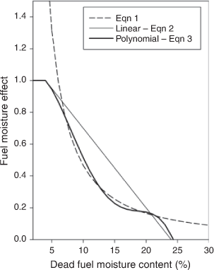
The Project Vesta experimental fires were conducted in a narrow MC range (McCaw et al. 2012), making it necessary to use a pre-defined fuel moisture effect function. In the current fire spread modelling context, a fuel moisture effect function is a mathematical description of the relationship between fuel moisture and rate of fire spread (Sullivan 2009). Cheney et al. (2012) used the equation developed by Burrows (1999) in developing their model. This function works well in the mid-range of MC but results in a steep effect under low dead fuel moisture conditions and asymptotes to a value around 0.1 for increasingly high fuel moisture contents (Fig. 1). Evidence from the analysis of various wildfire datasets by Cruz et al. (2020) suggest the effect of MC on rate of fire spread (R) flattens below a MC value of ~5% (i.e. decreasing fuel moisture below this level did not increase the R of wind-driven fires. In contrast, in the upper range of fuel moisture contents there exists a ‘moisture of extinction’ threshold (Rothermel 1972; Cheney 1981), above which the likelihood of fire spread decreases. Data from Gould (1994) and Cawson and Duff (2019) suggest that sustained fire propagation in eucalypt forests occurs at MC up to 20–25%.
|
We tested three MC effect functions (Fig. 1). As a benchmark, we used the Burrows (1999) function (ΦMdB) as per Cheney et al. (2012):
A second approach was to consider the effect of fuel moisture on rate of fire spread to be linear, as found in controlled experiments (e.g. Anderson 1964). The linear MC effect function (ΦMdL) was constrained to a value of 1.0 when MC ≤ 5% and zero when MC > 23.5%:
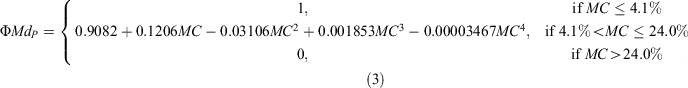
A third approach considered a polynomial equation form as per Rothermel (1972). The polynomial function (ΦMdP) was made to fit the Burrows (1999) function in the mid-range of MC, flattening to a value of 1.0 when MC ≤ 5%, and yielding a value of 0 when MC > 23.5%:
Effect of seasonal dryness – fuel availability
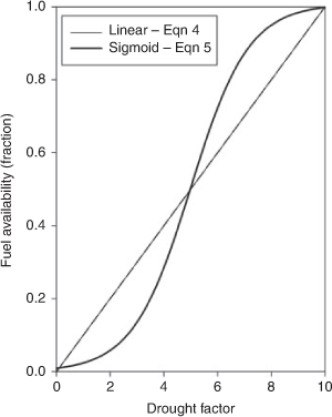
The moisture content of live and dead fuels with long time-lag responses were not measured comprehensively in the experimental fires or at all in the wildfires used in the present analysis. Although the direct linkages between the moisture content of these fuels and the spread rate of fires have not been clearly established, it is generally recognised that as these moisture contents decrease as a result of seasonal dryness, more fuels become available for combustion (Hollis et al. 2011), and in turn, fireline intensity and spread rate increases (Luke and McArthur 1978; Van Wagner 1998). We used McArthur (1967) drought factor (DF) as an approximation of the effect of fuel availability (FA) on the rate of fire spread, testing two equation forms. The first one follows McArthur (1967) linear relationship between DF and FA:

where ΦFA is the fuel availability function that varies between 0 and 1. This function implies that all fuel is available for combustion as the DF reaches its maximum value of 10. We also tested an alternative functional form that considers a sigmoid curve, as per the effect of curing in rate of fire spread in grasslands (Cheney et al. 1998). The sigmoid equation was fitted by forcing the curve through a FA of 0.5 and 1.0 at DF values of 5.0 and 10 respectively:
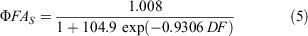
Figure 2 illustrates the differences between the two ΦFA functions, with the sigmoid function resulting in higher FA outputs when the DF is above 5.0.
|
The effect of fine dead fuel moisture, as expressed in Eqns 1–3, and long-term fuel dryness as expressed in Eqns 4–5, were integrated into an overall fuel moisture effect function (ΦM):

Fire behaviour modelling
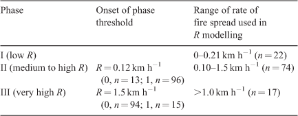
Based on the assumption that the rate of fire spread in eucalypt forests over its full range of occurrence cannot be adequately modelled using a single continuous equation, we postulate for practical purposes that there are three distinct phases of fire propagation: (1) a low-intensity state (henceforth called Phase I) associated with short flames consuming mostly surface and near surface fuels; (2) a moderate to high-intensity state (Phase II) involving all understorey fuels plus a proportion of bark fuels; and (3) a third, higher-intensity state (Phase III) associated with fires involving the full fuel complex and short- to medium-range spotting dynamics strongly influencing fire spread. The simplicity of empirically derived analytical equations for rate of fire spread requires that each phase be modelled separately, with each phase being described by one rate of fire spread equation.
We modelled the rate of fire spread using non-linear regression analysis. Models were of the form:

where R is rate of fire spread (km h−1), U is either the 10-m open wind speed or the within-stand wind speed measured at 2-m height above ground (U10 or U2, km h−1), ΦM is the fuel moisture effect function, Fi are fuel structure predictor variables and the lower case letters (a, b, c) are regression constants. Models were fitted using the nls function in R (R Core Team 2019).
To determine in which phase a fire is spreading (i.e. Phase I, II or III), we classified each data point according to a particular state or phase on the basis of its rate of fire spread, and used multiple logistic regression analyses to quantify the likelihood a fire is spreading in a given phase. The probability (P) that a fire is spreading in a certain state (i.e. Phase II or III) is given by:
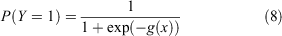
With the logit g(x) given by the equation:

with xi being the independent variables and βi the coefficients estimated through the maximum likelihood method. Model building using the glm function in R (R Core Team 2019) relied on stepwise procedures using the likelihood ratio Chi squared test and Wald test to access the significance of the coefficients. Model selection took into account the reduction in residual deviance from the null hypothesis as a measure of goodness-of-fit. This was supplemented by calculating Akaike’s Information Criterion (AIC) (Akaike 1974) and McFadden pseudo R2 statistic (McFadden 1974).
Model evaluation
The performance of a given rate of fire spread model was first assessed using the residual standard error (RSE), the significance of individual model parameters, the analysis of model behaviour outside the model development data range compared with expectations. Subsequently, promising models were evaluated through the calculation of the mean absolute error (MAE), the mean bias error (MBE), the mean absolute percentage error (MAPE) and the root mean squared error (RMSE) (Willmott 1982). Detailed evaluation was supplemented by the analysis of residual plots: residuals against fitted values, normal quantile plots of the residuals and residuals versus other variables.
Results
Study results are presented as follows: summary of characteristics of datasets used for model development; modelling the transitions between each fire spread phase; modelling the fire spread rate within each phase; linking of model components; and evaluation of the combined operational model.
Dataset characteristics
The assembled model development datasets for fire spread modelling, comprising data from Project Vesta experimental fires and the wildfires compiled by Cheney et al. (2012), were first constrained to reduce the uncertainty introduced into the analysis by variables such as slope angle, θ, and DF. We removed from the model development dataset fires that were characterised by a θ > |5°| and a DF < 9.0. A total of 87 experimental fires and 17 wildfires was then available for the modelling analysis (Table 2). The U10, MC and R variables in the experimental dataset varied between 7 and 23 km h−1, 5.6 and 9.4%, and 0.028 and 1.16 km h−1 respectively. For the wildfire dataset these same quantities varied between 10 and 72 km h−1, 2.8 and 8.6% (estimated MC), and 0.6 and 10.5 km h−1 respectively. U2 was measured in the experimental fires, and estimated from established wind reduction factors for the wildfire data.

|
The dry mass, or load (oven-dry weight basis), of surface fuels sensu McArthur and Luke (1963), comprising litter and near-surface fuels, constitute the bulk of understorey fine fuels in eucalypt forests (Luke and McArthur 1978; Gould et al. 2011). This is a common fuel metric used in Australia to describe fuel condition in eucalypt forests. This quantity varied between 0.66 and 2.18 kg m−2. On average, litter accounted for 72% of this fuel load metric. Near-surface fuel height varied between 0.05 and 0.5 m. Understorey fuel height (hu, m), defined as the average height (hi) of near-surface (lower shrubs and vertically oriented dead fuels) and elevated (taller shrubs) fuels weighted by their cover (Ci), was calculated as follows:

This fuel descriptor varied between 0.06 and 0.97 m in the experimental fire dataset and between 0.32 and 0.64 m in the wildfire dataset.
For model evaluation, the experimental fire data from the Project Aquarius (n = 14) had U10, MC and R variables varying between 8 and 19 km h−1, 4.6 and 9.7%, and 0.02 and 0.96 km h−1 respectively. Surface fuel load and understorey height averaged 2.1 kg m−2 and 0.42 m respectively. Of the 183 wildfire-spread observation periods (or ‘fire runs’) in the Southern Australia wildfire dataset, 90 were used in the analysis after removing runs of less than 1.0 h duration. Fire runs where propagation occurred immediately after the passage of a weather front over the fire area, a process that converts the pre-passage fire’s flank into a broad head fire, were also not considered in the evaluation (see Discussion). Of these 90 fire runs, 71 had a DF ≥ 9.0 (characteristic of dry summer conditions and reflecting a uniformly dry landscape) and 19 were characterised with a DF < 9.0. Wind speed and estimated fine dead fuel moisture content were comparable within the two subsets, varying between 12 and 100 km h−1 and 1.8 and 13.3% respectively (Table 2). Rates of forward spread were somewhat faster in the higher DF subset, averaging 2.37 km h−1, compared with 2.16 km h−1 for the lower DF subset. Surface fuel loads averaged 1.31 and 1.49 kg m−2 for the high and low DF subsets respectively.
Modelling the transition between phases
Exploratory analysis of the relationship between fire spread rates and intensity and wind speed in the model development dataset was used to define the range of each fire spread phase and the threshold values defining the transition between phases (Table 3). R was found to be a better discriminator to quantify the transition between phases than fireline intensity (Byram 1959). This was possibly due to the added uncertainty of what constitutes the available fuel load for the calculation of fireline intensity and the fact that R varies over a much wider range than fuel load (Alexander 1982).
|
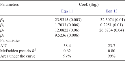
The best-fitting model for the transition of Phase I into Phase II had a threshold R of 0.12 km h−1 (Table 3), with U2, ΦM and Ws as significant variables (Table 4):

|
This model yielded a McFadden pseudo R2 of 0.62. The use of ΦM (p-value = 0.06) instead of the observed MC resulted in a better fit. Considering fuel structure variables, the use of other fuel variables in the model, such as litter fuel load, understorey fuel load or height, or fuel hazard scores, resulted in comparable coefficient significance and model fit. The use of a higher R threshold value for discriminating Phase I from Phase II, such as 0.18 or 0.24 km h−1, resulted in models with higher AICs and non-significant coefficients for the moisture content effect. The datasets available do not allow exploration of the impact of marginal fuel loads (e.g. < 0.1 kg m−2) on fire propagation. To ensure model outputs are consistent with expectations when fire is spreading where fuel quantity and structure limits the energy available to cause vertical fire transitions, the following condition is imposed:
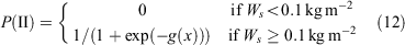
where P(II) is the probability of Phase II occurring and g(x) is the logit in Eqn 11.
The best-fitting models for the transition between Phase II and III were based on a threshold R of 1.5 km h−1. This threshold was largely dictated by the distribution of the rate of spread data, with all the Phase III data originating from wildfire case studies. The model for the onset of Phase III had wind speed, incorporated as U10, and ΦM, as significant variables (Table 4):

None of the available fuel variables was significant when further added to the model. This model resulted in a McFadden pseudo R2 of 0.80. As with Phase II transition, there are no data available to investigate the effect of the understorey fuel structure on the transition into Phase III when the fuel structure state limits this transition, as it would occur in the immediate years after an effective fuel reduction burn. To ensure the model does not identify Phase III fire propagation if understorey fire activity does not generate enough energy to generate the transition into this phase, the following constraint was applied:
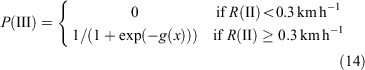
where P(III) is the probability of Phase III occurring and g(x) is the logit from Eqn 13.
Modelling fire spread rate within each phase
The observed rate of fire spread from the model development data was normalised to an equivalent θ and MC rate of fire spread (RAd, km h−1), as per Cheney et al. (2012):
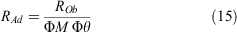
where ROb is the observed rate of fire spread and RAd is the adjusted rate of fire spread used as the dependent variable in the regression analysis. ΦM is given by Eqn 6 and Φθ is the effect of slope angle (θ) on fire spread rate as heuristically described by McArthur (1962, 1967) and parameterised by Noble et al. (1980):

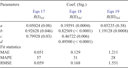
Modelling RAd tested the adequacy of the three different ΦMd functions as given in Eqns (1–3). In the following analysis we focus on the results of the models based on the ΦMdp function, as represented by Eqn 3, because this was found to produce the best results. Model parameterisations and fit for the models based on the other two ΦMd functions are given in the Supplementary Material (Tables S1–S5).
The model for R in Phase I (R(I)Ad) was fitted using data with R up to 0.21 km h−1 (Table 3). The best model had the form:

where Rt is a threshold rate of spread, estimated to be 0.03, added to the equation to account for the addition of a threshold understorey wind speed, Ut, to the equation. The equation was fitted with Ut of 1 km h−1. U2 is the understorey wind speed (km h−1) measured at a 2-m height in the forest, and Ws the load of surface and near surface fine fuels (kg m−2). Both parameters were significant at the 0.05 α level (Table 5). In this model, U2 was a better predictor of R(I)Ad than U10. The model produced an MAE of 0.051 km h−1 and a MAPE of 57% against the adjusted rate of fire spread. The b exponent in the equation with U2 had higher statistical significance than was found if U10 was used. The use or addition of other fuel parameters, such as understorey fuel height, shrub height and load, or bulk density, did not result in an improved model fit. The use of visual fuel hazard scores (FHS), such as the surface FHS or near-surface FHS (Gould et al. 2011), as explanatory variables in the model instead of Ws, resulted in a slight, but not significant, improvement in model fit. Equation 17 is applicable for U2 > 2 km h−1. When U2 < 2.0 km h−1, R(I)Ad is assumed to be 0.03 km h−1.
|
The model for rate of fire spread within Phase II was developed with experimental fire data within an R range between 0.10 and 1.5 km h−1. Following the form of Eqn 7, the best model for R(II)Ad had U2, and two fuel structure variables, Ws and understorey height (hu):

with hu defined as per Eqn 10. All parameters were statistically significant (Table 5). The effect of U2 and Ws in this model were not as strong as for the Phase I model, even if hu was not in the model. The MAE for R(II)Ad was 0.13 km h−1 with an associated MAPE of 31%, a reduction over the percentage error obtained for R(I)Ad.
Model fit for the Phase III R was based on a subset of the data with R > 1.0 km h−1. The best model form was:

with the U10 exponent being 1.19 (Table 5), a value higher than the exponents found for the Phase I and II models. No physical fuel structure parameters were found to be significant in this model. The use of fuel age as a surrogate for fuel condition was also found not to be significant. These results are consistent with the findings that fuel structure effects on fire spread decrease as fire weather become more severe (Tolhurst and McCarthy 2016; Cruz et al. 2020). U10 was chosen over U2 in this model because: (1) there were no accurate understorey wind measurements in most of the high-intensity wildfire data within this subset; and (2) the available wind reduction factors for the wildfire data were only estimated based on broad stand structure assumptions. It is also expected that fires spreading in Phase III involving the full fuel complex will be driven by the open wind rather than understorey winds. The MAE and MAPE for this model were 1.21 km h−1 and 28% respectively.
The application of models in Eqns 17–18 to predict R requires the addition of the effects of MC, FA and θ. The R of Phase i (I,…,III) is given by:

Model linkages
The prediction of R requires linking the transition likelihood models with the fire spread rate models developed for the three phases. The likelihood models define the weight each rate of fire spread model has on the rate of fire spread calculation for a given set of weather and fuel conditions. To avoid the abrupt changes in R that would occur if a fixed likelihood threshold was used to indicate a change from a lower to a higher state (e.g. using P(II) ≥ 0.5 to shift from R(I) to R(II)), or the inverse, the overall rate of fire spread output is a result of the value predicted by the R(i) models (Eqn 20) weighted by the likelihood of the fire is in that state. R is then given as:
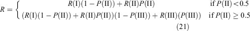
The application of Eqn 21 requires assumptions about the vertical wind profile. Considering U10 as the benchmark in a given wildfire prediction situation, U2 can be estimated from the appropriate wind reduction factor (WRF):

Appendix 1 provides guidance on the estimation of WRF for the range of forest cover and heights typical of Australian native eucalypt forests (Sneeuwjagt and Peet 1998; Moon et al. 2019).
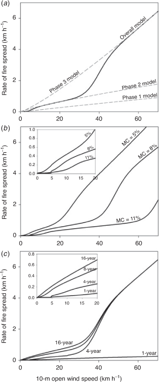
Figure 3a illustrates how R varies with U10 in Eqn 21 and contrasts with predictions for each spread phase as represented by Eqn 20. Figure 3b illustrates the effect of U10 and MC in the model outputs, from a low value of 5% as characteristic of extreme fire potential days to a relatively high value of 11%, typical of a mild burning day. Figure 3c shows the model response to changes in fuel structure by considering the effect of wind speed for four fuel ages (e.g. 1, 4, 8 and 16 years since a fuel reduction burn) on a dry eucalypt forest. For the very young fuels, the low available fuel load and the incipient understorey vegetation limit the energy release and the spread in Phase I and II, which then constrain the transition into Phase III, even under high wind speeds and low fuel moisture contents (MC = 7% in simulated example).
|
Model evaluation
Model fit against model development data
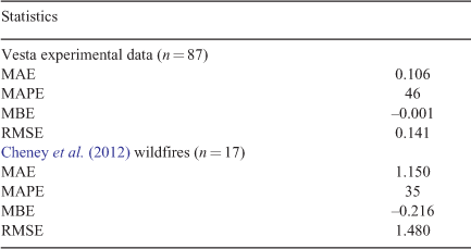
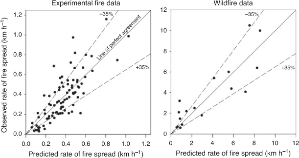
Table 6 provides goodness-of-fit metrics for Eqn 21 with the data used in the model development (Fig. 4). For the Project Vesta dataset, where the average R was 0.37 km h−1, the MAE was 0.106 km h−1. Mean bias was negligible, as expected from the application of the least square method, and MAPE was 46%. MAE for the wildfire dataset was one order of magnitude higher, at 1.15 km h−1 with a MAPE of 35%, a value lower than that obtained for the experimental fire dataset. The MBE for the wildfire subset was –0.216 km h−1, an under-prediction of less than 6% of the average R of 3.7 km h−1. Figure 4b shows the two fastest wildfire runs used in the model development, with R > 9.0 km h−1, were under predicted by the model. These two wildfires had documented spotting distances longer than 10 km observed during these fire runs. The fit statistics for the models developed with the two other MC effect functions, represented by Eqns 1 and 2, are to be found in the Supplementary Material (Tables S6, S7). As products of the same dataset, the fit statistics for the various model forms did not show notable differences.
|
|
Model fit against independent data
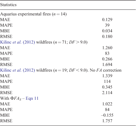
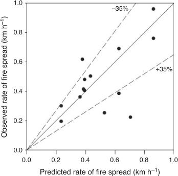
Model evaluation against the Project Aquarius dataset (average R = 0.47 km h−1) yielded an MAE, MAPE and MBE of 0.129 km h−1, 39% and 0.034 km h−1 respectively (Table 7). Ten of the 14 predictions were within the ± 35% error margin (Fig. 5) as ascribed by Cruz and Alexander (2013).
|
|
The partition of the Southern Australia wildfire dataset into two DF classes allowed for the separate evaluation of the fire spread model system for fuel conditions typical of a dry summer (i.e. high DF) and for conditions when the fuel availability is lower and the landscape is not homogeneously dry (i.e. lower DF). For the high DF subset, the model yielded an MAE, MAPE and MBE of 1.26 km h−1, 83%, and 0.266 km h−1 respectively. This MBE value corresponds to ~10% of the average R of the subset (i.e. 2.54 km h−1). This low bias is indicative of an overall unbiased prediction of the independent dataset (Table 7).
The evaluation against the low DF dataset allows one to understand how the implemented ΦFA reduces error relative to a situation where no FA function was implemented. The results showed the application of the ΦFAS to reduce the error relative to a scenario where no FA correction is applied (Table 7). Without the FA correction, the model produced an MAE of 1.339 km h−1, a MAPE of 114% and an over prediction bias of 0.345 km h−1. With the ΦFAS, the MAE was reduced to 1.022 km h−1 and the MAPE was 84%. The magnitude of the MBE was reduced to –0.155 km h−1 (Table 7). This MBE represented ~7% of the average R for the lower DF dataset, and 15% of the MAE. This evaluation of the ΦFAS, is restricted to DF values above 6.2, the lower limit of the DF in the dataset. The use of ΦFAS produced better results than the application of a linear FA correction ΦFAL as per Eqn 4.
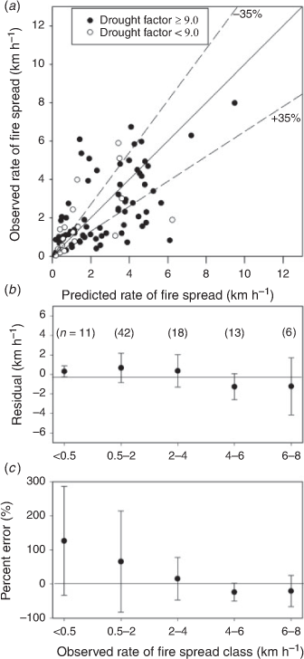
Figure 6a presents the observed versus predicted rates of fire spread for the independent model evaluation using the Southern Australia wildfire dataset (Kilinc et al. 2012). The figure shows a good number of observations were satisfactorily predicted within the ± 35% error band. The figure also shows several observations, 9 out of 90 or ~10% of the dataset, where the model either strongly over- or under-predicted the observed rates of fire spread. Given the inherent uncertainties in the wildfire data (Alexander and Cruz 2006), it is unclear if these notable errors are the result of a lack of representativeness in the measured weather conditions for the fire area, the uncertainty in the interpretation of fire perimeter location with time, model error, or the occurrence of other phenomena such as long-range spotting or fire–atmosphere interactions. We interpret these errors as ‘noise’ in the data due to these uncertainties.
|
Figure 6b, c provides an overview of the distribution of residuals and percentage error associated with the model predictions. Residuals were calculated as predicted minus observed, with negative residuals indicating an under-prediction. The predictions for fires with an observed rate of fire spread < 4 km h−1 indicate, on average, an over-prediction trend. Fires having an R > 4 km h−1 were, on average, under-predicted. Of the 20 observations within this condition, 14 (70%) were within the ± 35% error band. Error as a percentage of observed rate of fire spread was highest for the slowest spread rate class (i.e. < 0.5 km h−1, an average over-prediction of 126%). Percentage error decreased with increased rate of fire spread, with an average percentage error of 68% for wildfires spreading with R between 0.5–2.0 km h−1, and 20% for wildfires with R varying between 2.0 and 4.0 km h−1. For fires spreading with an R between 4.0–6.0 and 6.0–8.0 km h−1, the percentage error was –24% and –21% respectively.
Three of the four largest under-predictions (Fig. 6a) were characterised by open wind speeds above 40 km h−1 and relative humidity above 25%, a high value for severe fire behaviour in eucalypt forest. It is unclear if the high relative humidity was representative of the fire area or specific only to the immediate site of the measurement, but it was this variable and its effect on the moisture content of dead fuels that mostly contributed to the large under-prediction. Most of the larger over-predictions observed in the lower range of the observed rate of fire spread (Fig. 6a) were associated with morning or overnight fire runs under high wind speeds (i.e. U10 > 40 km h−1).
Discussion
Wind speed effect
The effect of wind speed is typically incorporated into models for the rate of fire spread through a power function, with the exponent varying around a value of 1.0 (Cheney et al. 1998; 2012; Anderson et al. 2015). The exponent is likely a function of not only the effect of wind on the heat transfer from the flame front into unburned fuels, but also the drag effect of overstorey and understorey vegetation on flame level wind flow and the distribution of the fire spread and wind data. In our analysis the wind exponent varied between 0.82 for the low-intensity Phase I and 1.19 for the high-intensity Phase III. The higher exponent found for the Phase III R model likely arises from the open nature of the U10 input and the effect of firebrand transport and spot fire ignition in driving headfire propagation in high-intensity wildfires in eucalypt forests. The 1.19 exponent makes the outputs of this model under high wind speeds and low fuel moisture contents up to 10% higher than the expectation of R being 10% of wind speed under extreme fire spread potential (Cruz and Alexander 2019).
The use of the fire spread model system described here requires knowledge of the wind speed at both the 10-m exposure standard (typically from a weather forecast) and in the understorey (assumed to be 2-m or eye-level height). Conversion between the U10 and U2 requires assumptions about the vertical wind profile under the canopy – a function of several factors, namely forest structure and canopy architecture, understorey development, atmosphere stability and wind speed itself (Moon et al. 2019). For an expedited model application, we provide a table of wind reduction factors allowing the direct conversion between U10 and U2 (Appendix 1). This table is a simplified first approximation. Customised wind profiles can be derived from large eddy simulation of wind flow within forest stands as per Pimont et al. (2009) and Mueller et al. (2014), for example.
Fuel moisture content effect
The effect of fuel moisture on the spread of fires is often portrayed as a well understood and well quantified process. However, this is far from the truth, likely due to the difficulty in controlling for fuel moisture over a relevant range and the fuel moisture gradients present in outdoor fires (Stocks 1970). Only a few studies have established relationships between fuel moisture controlled in a laboratory setting and rate of fire spread (Anderson 1964; Rothermel 1972). Results from field experiments by Burrows (1994) suggest this effect to be indeed linear for a range of fuel moisture contents, but a significant increase in rate of fire spread was observed in the lower fuel moisture levels. It is unclear if this escalation was due to fuel moisture itself or due to the involvement of additional fuel layers in the flame front as fireline intensity increased with the reduction of the fuel moisture content effect on fire spread rate. This bulk effect of fuel moisture content is frequently captured in fire spread models with a function that approximates an exponential decay (Fernandes et al. 2009; Sullivan 2009; Anderson et al. 2015) or with a polynomial function as done by Rothermel (1972). We tested different functions and found the polynomial form to work best. This effect is nonetheless still a simplification. Anderson and Rothermel (1965) and Burrows (1999) found the effect of fuel moisture to vary with wind speed, a detail we were unable to incorporate in our model due to the lack of data describing this behaviour. Similarly, we assume a nominal dead fuel moisture of extinction of 24% in the current model, but it is accepted that this value will vary with fuel structure, namely fuel bed porosity, and wind speed (Wilson 1985; Awad et al. 2020). With model fitting based on data in the lower range of the fuel moisture spectrum (i.e. <10%), changes to the fuel moisture function in the mid- to upper-range of the spectrum (if found necessary from future research work) will not affect the model formulation.
Similarly, advances in the understanding of the influence of the moisture content of live and dead fuels with longer time-lag response on fuel availability and fire behaviour in eucalypt forests can be incorporated in the ΦM without affecting the model presented here.
Estimating fine fuel moisture content and fuel availability
The fire spread model parameterisation was based on mid-afternoon experimental fires and fast-spreading wildfires burning within a homogeneously dry litter and duff layer profile. The simplified parameterisation of the Matthews (2006) process-based model used in the estimation of fine dead fuel moisture under wildfire conditions is known to give an unbiased prediction for dry, mid-afternoon conditions (Gould et al. 2007a). However, using this model with input data from a forecast or open weather station observations might not capture well the forest micro-climate environment during the mid-morning and early afternoon, after fuels have absorbed a significant amount of moisture overnight and before significant boundary layer mixing occurs. In these situations, the fuel moisture model will likely under-predict fuel moisture content (Slijepcevic et al. 2015). This might explain why the fire spread model showed an over-prediction trend for the wildfires spreading during the earlier part of the day. For those situations the application of a more detailed moisture estimation using Matthews (2006) model instead of a simplified derivation (as given in Gould et al. 2007b), taking into account fuel type specific parameterisations (Slijepcevic et al. 2013) and fuel level micro-meteorology inputs, will be required in order to obtain an unbiased input for the fire spread model.
The use of a fuel availability function based on the DF, an index calculated daily in Australia, is a pragmatic approach that enables an approximation of the effect of long-term dryness in determining fuel availability to be implemented for operational predictive purposes. Its implementation here led to a 30% reduction in average error for wildfires burning under low DF levels relative to predictions without the fuel availability function. Other, more comprehensive fuel availability functions exist that warrant future exploration, namely the Available Fuel Factor in the Western Australia Forest Fire Behaviour Tables (Beck 1995; Sneeuwjagt and Peet 1998). This factor requires knowledge of the moisture content of deep litter and duff fuel layers. These variables are not easily estimated and are typically not tracked or estimated on a daily basis in forest types in eastern Australia. The application of such fuel availability function would limit the use of the system for operational wildfire prediction until systematic and easily implemented models that represent the moisture dynamics of deep forest floor fuel layers are developed.
Fuel structure effect
The effect of fuel quantity and other fuel parameters on the spread rate of fires in eucalypt forests has been a contentious issue within the Australian fire behaviour modelling community. A directly proportional effect of fuel load on the speed a fire travels, with a doubling in fuel load leading to a doubling in rate of fire spread, was first suggested by McArthur (1962), based on data from low-intensity experimental fires. This direct effect has been at the foundation of fire spread modelling in Australia for many decades (McArthur 1967; Sneeuwjagt and Peet 1998). Nonetheless, this assumption has not held true in field studies of fires spreading with moderate to high intensities. Burrows (1994, 1999) did not find a significant relationship between fuel load and rate of fire spread in an experimental fire database with R values up to 0.6–0.7 km h−1, and reasoned that the direct relationship as proposed by McArthur (1962) is likely to be only valid for fires spreading under low wind speeds and without developing a definite headfire region. Gould et al. (2007a) found a variable effect of fuel load on rate of fire spread, with the effect being significant for low wind speeds, but non-significant as wind speed and rate of fire spread increased.
Our phased modelling analysis produced similar results, with the load of the surface and near-surface fuels having an almost direct effect on the spread rate of Phase I fires. For Phase II, the main fuel effect was described by the understorey fuel height, although the fuel load still had an effect, albeit lower than for Phase I. Although fuel structure was not found to contribute or influence the rate of fire spread for the faster-spreading fires in Phase III (R > 1.5 km h−1), spread in this phase is dependent on the presence of an understorey fuel layer or ladder fuels (e.g. fibrous bark) sufficient to produce flames that allow for the vertical transition of fire into the crowns (i.e. no fuel, no fire). A typical eucalypt forest will not support a Phase III fire when understorey fuels have been removed by prescribed burning. Fuels in eucalypt forests do recover quickly after a burn as a function of site productivity, stand structure and fire intensity (Peet 1971; Walker 1981). For example, in Western Australian forests, bulk density of near-surface fuels will typically reach 80% of the equilibrium level within 4 years (Gould et al. 2007a). Consistent with the findings for the rate of fire spread equations, fuel load is an influential variable for the logistic equation predicting the likelihood a fire will spread in Phase II, but not for the transition to Phase III.
The quantity of surface and near-surface fuels is a commonly assessed variable in fuel inventory studies in Australia, and a wealth of information exists on its characterisation, relationships with vegetation or fuel types, and modelling (Walker 1981; Watson et al. 2012). However, the fuel that determines how fast a fire spreads is the fuel that is consumed by the flames at the leading edge of the head fire. As the fire increases in intensity it integrates the fuel consumed over an increasingly large volume. Only an unknown fraction of the total fuel consumed is involved in the flaming combustion processes that drive heat transfer into unburned fuels (Gould et al. 2007a). So although we can describe the fuel consumed in the overall combustion process, we cannot accurately define or measure the fuel contributing to the flame front. Our findings suggest that the best fuel descriptor from the point of view of the operational prediction of fire spread is the height of the understorey fuels. This variable is defined as the average height of both the near-surface and elevated fuels weighted by their cover on a per area basis. This metric quantifies the volume of fuels per unit area. It can be derived from simple estimates of height and cover, or through remote sensing of fuels using LIDAR (Skowronski et al. 2014; Price and Gordon 2016; Hillman et al. 2021). Work is under way to provide guidance to its estimation and derive landscape maps from knowledge of other commonly accessed fuel characteristics, such as fuel hazard ratings.
The use of visual hazard scores, such as those used in Cheney et al. (2012), resulted in a small improvement in the fit of fire spread rate models for Phase I and II. Nonetheless, this improvement did not warrant its use in the models due to the subjectivity inherent to their estimation (Duff et al. 2017).
Spotting
Spotting, or the process of transport of firebrands and the ignition of new fires outside the active fire perimeter, is a complex, poorly understood and quantified phenomenon that can have an important influence on wildfire propagation. It is an inherent feature of wildfire propagation in eucalypt forests (Cheney and Bary 1969; Luke and McArthur 1978; Ellis 2013). Spotting, either short- (up to 0.75 km by Australian standards) or medium-range (up to 5 km), was present in the model development data and is thus implicit in the model system described herein. Longer spotting distances (i.e. >5 km) occur under severe fire weather conditions in Australian eucalypt forests (McArthur 1969; Rawson et al. 1983; Storey et al. 2020a). The influence of these longer spotting distances on a wildfire’s overall propagation rate is unclear. For a newly ignited spot fire occurring ahead of a wildfire to spread independently and result in an increased R relative to the model expectation, it will need to land in an area where wind flow is not influenced by the convection column. Often, spot fires initiating downwind of a fire within the plume wake region (Forthofer and Goodrick 2016) spread without a general direction (see fig. 4 in Storey et al. 2020b). These spot fires will be overrun by the main fire without resulting in an increase in the overall speed a wildfire propagates. It is unclear what is the extent and width of this plume wake region for a given combination of fire size and energy release, environmental conditions, and associated fire–atmosphere interactions. It is also unclear, therefore, what the necessary maximum spotting distance is for a long-range spot fire to grow and increase the overall propagation speed of the wildfire beyond the model expectation. The occurrence of such spot fires can result in a model under-prediction.
Model fit and operational considerations
The models developed here are intended for use in the operational prediction of wildfire propagation in eucalypt forests over a broad range of fireline intensities. They assume a pseudo-steady-state has been achieved and aim to predict fire spread over time scales of one or more hours, based on observed or forecasted weather conditions. Their application to fire spread periods of less than 30 min is likely not to accurately capture the finer-scale variability in observed fire behaviour. The models do not capture fire spread dynamics associated with the passage of a cold front or wind change over the fire area, a process that converts a fire’s flank into a broad head fire (Luke and McArthur 1978; Cheney et al. 2001). This is a poorly understood process, with the post change area growth typically unrelated to the prevailing wind strength and the air mass high relative humidity (McArthur 1967).
Average model error against independent evaluation data varied between 39% for experimental fire data (where accurate estimates of input conditions are known) and 84% for wildfires with larger uncertainty in model inputs. This level of error is consistent, although lower, than the results obtained with other empirically based fire spread models evaluated against wildfire data (Cheney et al. 2012; Cruz and Alexander 2013). An important result from the present work is that the percentage error decreased with an increase in observed rate of fire spread, suggesting that the model works best for the conditions in which it will be most needed.
It is believed that in an operational fire prediction scenario, trained fire behaviour analysts will be able to produce more accurate predictions than reported here. Fire behaviour prediction is both an art and a science, combining the use of models with tailored spot fire weather forecasts and the shared experience of a cadre of qualified users with knowledge of landscape factors and fire processes that are not explicit in the models (Neale and May 2020).
The unquantified effects of the occurrence of long-range spotting and fire–atmosphere interactions (Cheney et al. 2012; Fromm et al. 2012; McRae et al. 2015; Sharples et al. 2016) on the precision of model predictions is unclear. Detailed evaluation against several fires known to have exhibited these kind of fire phenomena is required in order to further understand model adequacy/limitations in these situations. Similarly, the evaluation of the models for the marginal- to low-intensity spread conditions characteristic of prescribed burns and overnight fire activity under mild burning conditions is also required.
Concluding remarks
We developed a fire spread model aimed at the operational prediction of the steady-state propagation of wildfires in eucalypt forests. The model blends empirical data covering a broad spectrum of rates of fire spread with assumptions of fire behaviour from published studies. The model was shown to provide adequate predictions when contrasted with independent wildfire data, with the percentage error decreasing with increasing observed rate of fire spread. Evaluation highlighted areas where further submodelling, for example dealing with overnight recovery of dead fuel moisture content, could potentially lead to an improvement in the overall application of the model.
With the model being based on a broad range of rates of fire spread, comprising experimental fires and wildfires, we see its predictions as an expectation of fire spread rates associated with the prevailing environmental conditions. There is natural uncertainty associated with the model, derived from the uncertainty in the experimental fire and wildfire data and the simplicity and coarseness of how the model incorporates the effect of various environmental effects. When the model is used in an operational wildfire prediction setting, the uncertainty inherent in the model will be increased due to the uncertainty in the forecasted (e.g. wind speed and direction, dead fuel moisture content) and modelled (e.g. fuel structure from time since fire) inputs. Uncertainty and errors in model outputs can be reduced from the benchmark results obtained here when predictions are made by qualified and experienced fire behaviour analysts.
Data availability
The data that support this study will be shared upon reasonable request to the corresponding author.
Conflicts of interest
Lachlan McCaw and Andrew Sullivan are Associate Editors of International Journal of Wildland Fire, but were blinded from the peer-review process for this paper.
Declaration of funding
This project was collaboratively funded by the New South Wales Rural Fire Service and the Commonwealth Scientific and Industrial Research Organisation through research agreement 2019051144.
Acknowledgements
We thank the State Government of New South Wales and CSIRO for funding this project. We also thank Marty Alexander and Stuart Matthews for their comments on a draft of this manuscript.
References
Akaike H (1974) A new look at the statistical model identification. IEEE Transactions on Automatic Control 19, 716–723.| A new look at the statistical model identification.Crossref | GoogleScholarGoogle Scholar |
Alexander ME (1982) Calculating and interpreting forest fire intensities. Canadian Journal of Botany 60, 349–357.
| Calculating and interpreting forest fire intensities.Crossref | GoogleScholarGoogle Scholar |
Alexander ME, Cruz MG (2006) Evaluating a model for predicting active crown fire rate of spread using wildfire observations. Canadian Journal of Forest Research 36, 3015–3028.
| Evaluating a model for predicting active crown fire rate of spread using wildfire observations.Crossref | GoogleScholarGoogle Scholar |
Anderson HE (1964) Mechanisms of fire spread research progress report No. 1. USDA Forest Service Intermountain Forest and Range Experiment Station, Research Paper INT-8. (Ogden, UT).
Anderson HE, Rothermel RC (1965) Influence of moisture and wind on the characteristics of free burning fires. Symposium (International) on Combustion 10, 1009–1019.
| Influence of moisture and wind on the characteristics of free burning fires.Crossref | GoogleScholarGoogle Scholar |
Anderson WR, Cruz MG, Fernandes PM, McCaw L, Vega JA, Bradstock RA, Fogarty L, Gould J, McCarthy G, Marsden-Smedley JB, Matthews S, Mattingley G, Pearce HG, van Wilgen BW (2015) A generic, empirical-based model for predicting rate of fire spread in shrublands. International Journal of Wildland Fire 24, 443–460.
| A generic, empirical-based model for predicting rate of fire spread in shrublands.Crossref | GoogleScholarGoogle Scholar |
Awad C, Morvan D, Rossi J-L, Marcelli T, Chatelon FJ, Morandini F, Balbi J-H (2020) Fuel moisture content threshold leading to fire extinction under marginal conditions. Fire Safety Journal 118, 103226
| Fuel moisture content threshold leading to fire extinction under marginal conditions.Crossref | GoogleScholarGoogle Scholar |
Beck JA (1995) Equations for the forest fire behaviour tables for Western Australia. CALMscience 1, 325–348.
Burrows ND (1994) Experimental development of a fire management model for jarrah (Eucalyptus marginata Donn ex Sm.) forests. PhD thesis, Australian National University.
Burrows ND (1999) Fire behaviour in jarrah forest fuels: 2 Field experiments. CALMscience 3, 57–84.
Burrows ND, Sneeuwjagt RJ (1991) McArthur’s forest fire danger meter and the forest fire behaviour tables for Western Australia, derivation, applications and limitations. In ‘Proceedings of Conference on Bushfire Modelling and Fire Danger Rating Systems. Yarralumla, ACT’, 11–12 July 1988. (Eds NP Cheney, AM Gill) pp. 65–78. (CSIRO Division of Forestry: Canberra, ACT)
Burrows ND, Ward B, Robinson A (1988) ‘Aspects of fire behaviour and fire suppression in a Pinus pinaster plantation.’ (Department of Conservation & Land Management)
Byram GM (1959) Combustion of forest fuels. In ‘Forest Fire: Control and Use’. (Ed. KP Davis). pp. 61–89. (McGraw-Hill, New York, NY)
Cawson JG, Duff TJ (2019) Forest fuel bed ignitability under marginal fire weather conditions in Eucalyptus forests. International Journal of Wildland Fire 28, 198–204.
| Forest fuel bed ignitability under marginal fire weather conditions in Eucalyptus forests.Crossref | GoogleScholarGoogle Scholar |
Cheney NP (1981) Fire behaviour. In ‘Fire and the Australian Biota’. (Eds AM Gill, RH Groves, IR Noble) pp. 151–175. (Australian Academy of Science, Canberra, ACT)
Cheney NP, Bary GAV (1969) ‘The propagation of mass conflagrations in a standing eucalypt forest by the spotting process’. Paper A6. In ‘Mass Fire Symposium’ 10–12 February 1969. (The Technical Cooperation Program, Defence Standard Laboratories: Melbourne)
Cheney NP, Gould JS, Catchpole WR (1993) The influence of fuel, weather and fire shape variables on fire-spread in grasslands. International Journal of Wildland Fire 3, 31–44.
| The influence of fuel, weather and fire shape variables on fire-spread in grasslands.Crossref | GoogleScholarGoogle Scholar |
Cheney NP, Gould JS, Catchpole WR (1998) Prediction of fire spread in grasslands. International Journal of Wildland Fire 8, 1–13.
| Prediction of fire spread in grasslands.Crossref | GoogleScholarGoogle Scholar |
Cheney NP, Gould JS, McCaw WL (2001) The dead-man zone – a neglected area of firefighter safety. Australian Forestry 64, 45–50.
| The dead-man zone – a neglected area of firefighter safety.Crossref | GoogleScholarGoogle Scholar |
Cheney NP, Gould JS, McCaw WL, Anderson WR (2012) Predicting fire behaviour in dry eucalypt forest in southern Australia. Forest Ecology and Management 280, 120–131.
| Predicting fire behaviour in dry eucalypt forest in southern Australia.Crossref | GoogleScholarGoogle Scholar |
Cruz MG, Alexander ME (2013) Uncertainty associated with model predictions of surface and crown fire rates of spread. Environmental Modelling & Software 47, 16–28.
| Uncertainty associated with model predictions of surface and crown fire rates of spread.Crossref | GoogleScholarGoogle Scholar |
Cruz MG, Alexander ME (2019) The 10% wind speed rule of thumb for estimating a wildfire’s forward rate of spread in forests and shrublands. Annals of Forest Science 76, 44
| The 10% wind speed rule of thumb for estimating a wildfire’s forward rate of spread in forests and shrublands.Crossref | GoogleScholarGoogle Scholar |
Cruz MG, Gould JS, Alexander ME, Sullivan AL, McCaw WL, Matthews S (2015) Empirical-based models for predicting head-fire rate of spread in Australian fuel types. Australian Forestry 78, 118–158.
| Empirical-based models for predicting head-fire rate of spread in Australian fuel types.Crossref | GoogleScholarGoogle Scholar |
Cruz MG, Alexander ME, Fernandes PM, Kilinc M, Sil  (2020) Evaluating the 10% wind speed rule of thumb for estimating a wildfire’s forward rate of spread against an extensive independent set of observations. Environmental Modelling & Software 133, 104818
| Evaluating the 10% wind speed rule of thumb for estimating a wildfire’s forward rate of spread against an extensive independent set of observations.Crossref | GoogleScholarGoogle Scholar |
Doogan M (2006) The Canberra Fire Storm. Inquests and Inquiry into Four Deaths and Four Fires Between 8 and 18 January 2003. Volume 1. (ACT Coroners Court: Canberra, ACT)
Duff T, Keane R, Penman TD, Tolhurst K (2017) Revisiting Wildland Fire Fuel Quantification Methods: The Challenge of Understanding a Dynamic, Biotic Entity. Forests 8, 351
| Revisiting Wildland Fire Fuel Quantification Methods: The Challenge of Understanding a Dynamic, Biotic Entity.Crossref | GoogleScholarGoogle Scholar |
Ellis PFM (2013) Firebrand characteristics of the stringy bark of messmate (Eucalyptus obliqua) investigated using non-tethered samples. International Journal of Wildland Fire 22, 642–651.
| Firebrand characteristics of the stringy bark of messmate (Eucalyptus obliqua) investigated using non-tethered samples.Crossref | GoogleScholarGoogle Scholar |
Fernandes PM, Botelho HS, Rego FC, Loureiro C (2009) Empirical modelling of surface fire behaviour in maritime pine stands. International Journal of Wildland Fire 18, 698–710.
| Empirical modelling of surface fire behaviour in maritime pine stands.Crossref | GoogleScholarGoogle Scholar |
Forthofer JA, Goodrick SL (2016) Vortices and Wildland Fire. In: Synthesis of Knowledge of Extreme Fire Behavior: Volume 2 for Fire Behavior Specialists, Researchers and Meteorologists. US Department of Agriculture, Forest Service, Pacific Northwest Research Station, Portland, OR, pp. 89–105. General Technical Report PNW-GTR-891.
Fromm MD, McRae RHD, Sharples JJ, Kablick GP (2012) Pyrocumulonimbus pair in Wollemi and Blue Mountains National Parks, 22 November 2006. Australian Meteorological and Oceanographic Journal 62, 117–126.
| Pyrocumulonimbus pair in Wollemi and Blue Mountains National Parks, 22 November 2006.Crossref | GoogleScholarGoogle Scholar |
Gibos KE, Slijepcevic A, Wells T, Fogarty L (2015) Building Fire Behavior Analyst (FBAN) Capability and Capacity: Lessons Learned From Victoria, Australia’s Bushfire Behavior Predictive Services Strategy. In ‘Proceedings of the large wildland fires conference’ 19–23 May, 2014. (Eds RE Keane, M Jolly, R Parsons, K Riley) Missoula, MT. (RMRS-P-73). Fort Collins, CO: U.S. Department of Agriculture, Forest Service, Rocky Mountain Research Station. 345 p.
Gould JS (1994) Evaluation of McArthur’s control burning guide in regrowth Eucalyptus sieberi. Australian Forestry 57, 86–93.
| Evaluation of McArthur’s control burning guide in regrowth Eucalyptus sieberi.Crossref | GoogleScholarGoogle Scholar |
Gould JS, Cheney NP, Hutchings PT, Cheney S (1996) Final Report on Prediction of Bushfire Spread for Australian Co-Ordination Committee International Decade of Natural Disaster Reduction (IDNDR). Project: 4/95. CSIRO Forestry and Forest Products, Bushfire Behaviour and Management Group.
Gould JS, McCaw WL, Cheney NP, Ellis PF, Knight IK, Sullivan AL (2007a) Project Vesta: Fire in Dry Eucalypt Forest: Fuel Structure, Fuel Dynamics and Fire Behaviour. Ensis-CSIRO, Canberra, ACT and Department of Environment and Conservation, Perth, WA.
Gould JS, McCaw WL, Cheney NP, Ellis PF, Matthews S (2007b) Field Guide: Fuel Assessment and Fire Behaviour Prediction in Dry Eucalypt Forest, Interim edition. (CSIRO Publishing: Melbourne)
Gould JS, McCaw WL, Cheney NP (2011) Quantifying fine fuel dynamics and structure in dry eucalypt forest (Eucalyptus marginata) in Western Australia for fire management. Forest Ecology and Management 262, 531–546.
| Quantifying fine fuel dynamics and structure in dry eucalypt forest (Eucalyptus marginata) in Western Australia for fire management.Crossref | GoogleScholarGoogle Scholar |
Harris S, Anderson WR, Kilinc M, Fogarty L (2011) Establishing a link between the power of fire and community loss: The first step towards developing a bushfire severity scale. Department of Sustainability and Environment Research report No. 89, Melbourne.
Hillman S, Wallace L, Lucieer A, Reinke K, Turner D, Jones S (2021) A comparison of terrestrial and UAS sensors for measuring fuel hazard in a dry sclerophyll forest. International Journal of Applied Earth Observation and Geoinformation 95, 102261
| A comparison of terrestrial and UAS sensors for measuring fuel hazard in a dry sclerophyll forest.Crossref | GoogleScholarGoogle Scholar |
Hollis JJ, Matthews S, Ottmar RD, Prichard SJ, Slijepcevic A, Burrows ND, Ward B, Tolhurst KG, Anderson WR, Gould JS (2010) Testing woody fuel consumption models for application in Australian southern eucalypt forest fires. Forest Ecology and Management 260, 948–964.
| Testing woody fuel consumption models for application in Australian southern eucalypt forest fires.Crossref | GoogleScholarGoogle Scholar |
Hollis JJ, Matthews S, Anderson WR, Cruz MG, Burrows ND (2011) Behind the flaming zone: predicting woody fuel consumption in eucalypt forest fires in southern Australia. Forest Ecology and Management 261, 2049–2067.
| Behind the flaming zone: predicting woody fuel consumption in eucalypt forest fires in southern Australia.Crossref | GoogleScholarGoogle Scholar |
Kilinc M, Anderson W, Price B (2012) The Applicability of Bushfire Behaviour Models in Australia. Victorian Government, Department of Sustainability and Environment, DSE Schedule 5: Fire Severity Rating Project, Melbourne, VIC. Technical Report 1.
Luke RH, McArthur AG (1978) Bushfires in Australia. Australian Government Publishing Service, Canberra, ACT.
Matthews S (2006) A process-based model of fine fuel moisture. International Journal of Wildland Fire 15, 155–168.
| A process-based model of fine fuel moisture.Crossref | GoogleScholarGoogle Scholar |
Matthews S, Gould JS, McCaw WL (2010) Simple models for predicting dead fuel moisture in eucalyptus forests. International Journal of Wildland Fire 19, 459–467.
| Simple models for predicting dead fuel moisture in eucalyptus forests.Crossref | GoogleScholarGoogle Scholar |
McArthur AG (1962) Control Burning in Eucalypt Forests. Commonwealth of Australia, Forestry and Timber Bureau, Forest Research Institute, Canberra, ACT. Leaflet 80.
McArthur AG (1967) Fire Behaviour in Eucalypt Forests. Commonwealth of Australia, Forestry and Timber Bureau, Canberra, ACT. Leaflet 107.
McArthur AG (1969) The fire control problem and fire research in Australia. In ‘Proceedings of the 1966 Sixth world forestry congress’, vol. 2. pp. 1986–1991. (FAO and Spanish Minister of Agriculture)
McArthur AG, Luke RH (1963) Fire behaviour studies in Australia. Fire Control Notes 24, 87–92.
McCaw WL, Gould JS, Cheney NP (2008) Existing fire behaviour models under-predict the rate of spread of summer fires in open jarrah (Eucalyptus marginata) forest. Australian Forestry 71, 16–26.
| Existing fire behaviour models under-predict the rate of spread of summer fires in open jarrah (Eucalyptus marginata) forest.Crossref | GoogleScholarGoogle Scholar |
McCaw WL, Gould JS, Cheney NP, Ellis PFM, Anderson WR (2012) Changes in behaviour of fire in dry eucalypt forest as fuel increases with age. Forest Ecology and Management 271, 170–181.
| Changes in behaviour of fire in dry eucalypt forest as fuel increases with age.Crossref | GoogleScholarGoogle Scholar |
McFadden D (1974) Conditional logit analysis of qualitative choice behavior. In ‘Frontiers in Econometrics’. (Ed P Zarembka) pp. 104–142. (Academic Press, New York)
McLeod R (2003) Inquiry into the Operational Response to the January 2003 Bushfires in the ACT. ACT Government Publication No. No 03/0537, Canberra.
McRae RHD, Sharples JJ, Fromm M (2015) Linking local wildfire dynamics to pyroCb development. Natural Hazards and Earth System Sciences 15, 417–428.
| Linking local wildfire dynamics to pyroCb development.Crossref | GoogleScholarGoogle Scholar |
Miller C, Hilton J, Sullivan AL, Prakash M (2015) SPARK – A Bushfire Spread Prediction Tool. In ‘Environmental Software Systems. Infrastructures, Services and Applications’. (Eds R Denzer, R Argent, G Schimak, J Hřebíček) Vol. 448. pp. 262–271. (Springer International Publishing)
Moon K, Duff TJ, Tolhurst KG (2019) Sub-canopy forest winds: understanding wind profiles for fire behaviour simulation. Fire Safety Journal 105, 320–329.
| Sub-canopy forest winds: understanding wind profiles for fire behaviour simulation.Crossref | GoogleScholarGoogle Scholar |
Mueller E, Mell W, Simeoni A (2014) Large eddy simulation of forest canopy flow for wildland fire modeling. Canadian Journal of Forest Research 44, 1534–1544.
| Large eddy simulation of forest canopy flow for wildland fire modeling.Crossref | GoogleScholarGoogle Scholar |
Neale T, May D (2018) Bushfire simulators and analysis in Australia: insights into an emerging sociotechnical practice. Environmental Hazards 17, 200–218.
| Bushfire simulators and analysis in Australia: insights into an emerging sociotechnical practice.Crossref | GoogleScholarGoogle Scholar |
Neale T, May D (2020) Fuzzy boundaries: Simulation and expertise in bushfire prediction. Social Studies of Science 50, 837–859.
| Fuzzy boundaries: Simulation and expertise in bushfire prediction.Crossref | GoogleScholarGoogle Scholar | 32053028PubMed |
Noble IR, Bary GAV, Gill AM (1980) McArthur’s fire danger meters expressed as equations. Australian Journal of Ecology 5, 201–203.
| McArthur’s fire danger meters expressed as equations.Crossref | GoogleScholarGoogle Scholar |
Peet GB (1971) Litter accumulation in jarrah and karri forests. Australian Forestry 35, 258–262.
| Litter accumulation in jarrah and karri forests.Crossref | GoogleScholarGoogle Scholar |
Pimont F, Dupuy JL, Linn RR, Dupont S (2009) Validation of FIRETEC wind-flows over a canopy and a fuel-break. International Journal of Wildland Fire 18, 775–790.
| Validation of FIRETEC wind-flows over a canopy and a fuel-break.Crossref | GoogleScholarGoogle Scholar |
Plucinski MP, Sullivan AL, Rucinski CJ, Prakash M (2017) Improving the reliability and utility of operational bushfire behaviour predictions in Australian vegetation. Environmental Modelling & Software 91, 1–12.
| Improving the reliability and utility of operational bushfire behaviour predictions in Australian vegetation.Crossref | GoogleScholarGoogle Scholar |
Price OF, Gordon CE (2016) The potential for LiDAR technology to map fire fuel hazard over large areas of Australian forest. Journal of Environmental Management 181, 663–673.
| The potential for LiDAR technology to map fire fuel hazard over large areas of Australian forest.Crossref | GoogleScholarGoogle Scholar | 27558828PubMed |
R Core Team (2019) R: A Language and Environment for Statistical Computing. R Foundation for Statistical Computing, Vienna, Austria.
Rawson RP, Billing PR, Duncan SF (1983) The 1982–83 forest fires in Victoria. Australian Forestry 46, 163–172.
| The 1982–83 forest fires in Victoria.Crossref | GoogleScholarGoogle Scholar |
Rothermel RC (1972) A Mathematical Model for Predicting Fire Spread in Wildland Fuels. US Department of Agriculture, Forest Service, Intermountain Forest and Range Experiment Station, Ogden, UT. Research Paper INT-115.
Sharples JJ, Cary GJ, Fox-Hughes P, Mooney S, Evans JP, Fletcher M-S, Fromm M, Grierson PF, McRae R, Baker P (2016) Natural hazards in Australia: extreme bushfire. Climatic Change 139, 85–99.
| Natural hazards in Australia: extreme bushfire.Crossref | GoogleScholarGoogle Scholar |
Skowronski NS, Clark KL, Gallagher M, Birdsey RA, Hom JL (2014) Airborne laser scanner-assisted estimation of aboveground biomass change in a temperate oak–pine forest. Remote Sensing of Environment 151, 166–174.
| Airborne laser scanner-assisted estimation of aboveground biomass change in a temperate oak–pine forest.Crossref | GoogleScholarGoogle Scholar |
Slijepcevic A, Tolhurst KG, Fogarty L (2008) Fire behaviour analyst roles and responsibilities in bushfire management-how to make the best use of these skills. In ‘Australian Fire and Emergency Services Authorities Council Conference’. Adelaide, South Australia. (AFAC)
Slijepcevic A, Anderson WR, Matthews S (2013) Testing existing models for predicting hourly variation in fine fuel moisture in eucalypt forests. Forest Ecology and Management 306, 202–215.
| Testing existing models for predicting hourly variation in fine fuel moisture in eucalypt forests.Crossref | GoogleScholarGoogle Scholar |
Slijepcevic A, Anderson WR, Matthews S, Anderson DH (2015) Evaluating models to predict daily fine fuel moisture content in eucalypt forest. Forest Ecology and Management 335, 261–269.
| Evaluating models to predict daily fine fuel moisture content in eucalypt forest.Crossref | GoogleScholarGoogle Scholar |
Sneeuwjagt RJ, Peet GB (1998) Forest Fire Behaviour Tables for Western Australia, 3rd edn. Department of Conservation and Land Management, Perth, WA.
Stocks BJ (1970) Moisture in the forest floor- its distribution and movement. Department of fisheries and forestry, Canadian Forestry Service Publication No. No. 1271, Ottawa.
Storey MA, Price OF, Sharples JJ, Bradstock RA (2020a) Drivers of long-distance spotting during wildfires in south-eastern Australia. International Journal of Wildland Fire 29, 459–472.
| Drivers of long-distance spotting during wildfires in south-eastern Australia.Crossref | GoogleScholarGoogle Scholar |
Storey MA, Price OF, Bradstock RA, Sharples JJ (2020b) Analysis of Variation in Distance, Number, and Distribution of Spotting in Southeast Australian Wildfires. Fire (Basel, Switzerland) 3, 10
| Analysis of Variation in Distance, Number, and Distribution of Spotting in Southeast Australian Wildfires.Crossref | GoogleScholarGoogle Scholar |
Sullivan AL (2009) Wildland surface fire spread modelling, 1990–2007. 2: Empirical and quasi-empirical models. International Journal of Wildland Fire 18, 369–386.
| Wildland surface fire spread modelling, 1990–2007. 2: Empirical and quasi-empirical models.Crossref | GoogleScholarGoogle Scholar |
Teague B, McLeod R, Pascoe S (2010) 2009 Victorian Bushfires Royal Commission Final Report. State of Victoria, Melbourne.
Tolhurst KG, McCarthy G (2016) Effect of prescribed burning on wildfire severity: a landscape-scale case study from the 2003 fires in Victoria. Australian Forestry 79, 1–14.
| Effect of prescribed burning on wildfire severity: a landscape-scale case study from the 2003 fires in Victoria.Crossref | GoogleScholarGoogle Scholar |
Tolhurst KG, Shields B, Chong D (2008) Phoenix: development and application of a bushfire risk management tool. Australian Journal of Emergency Management 23, 47–54.
Van Wagner CE (1968) Fire behaviour mechanisms in a red pine plantation: field and laboratory evidence. Canadian Department of Forestry and Rural Development Publication No. 1229.
Van Wagner CE (1998) Modelling logic and the Canadian forest fire behavior prediction system. Forestry Chronicle 74, 50–52.
| Modelling logic and the Canadian forest fire behavior prediction system.Crossref | GoogleScholarGoogle Scholar |
Walker J (1981) Fuel dynamics in Australian vegetation. In ‘Fire and the Australian biota’. (Eds AM Gill, RH Groves, IR Noble) pp. 101–28. (Australian Academy of Science: Canberra)
Watson PJ, Penman SH, Bradstock RA (2012) A comparison of bushfire fuel hazard assessors and assessment methods in dry sclerophyll forest near Sydney, Australia. International Journal of Wildland Fire 21, 755–763.
| A comparison of bushfire fuel hazard assessors and assessment methods in dry sclerophyll forest near Sydney, Australia.Crossref | GoogleScholarGoogle Scholar |
Whittaker J, Taylor M, Bearman C (2020) Why don’t bushfire warnings work as intended? Responses to official warnings during bushfires in New South Wales, Australia. International Journal of Disaster Risk Reduction 45, 101476
| Why don’t bushfire warnings work as intended? Responses to official warnings during bushfires in New South Wales, Australia.Crossref | GoogleScholarGoogle Scholar |
Willmott CJ (1982) Some comments on the evaluation of model performance. Bulletin of the American Meteorological Society 63, 1309–1313.
| Some comments on the evaluation of model performance.Crossref | GoogleScholarGoogle Scholar |
Wilson RA (1985) Observations of extinction and marginal burning states in free burning porous fuel beds. Combustion Science and Technology 44, 179–193.
| Observations of extinction and marginal burning states in free burning porous fuel beds.Crossref | GoogleScholarGoogle Scholar |
Appendix 1. Wind reduction factors (WRF) to convert 10-m open into 2-m within-stand wind for eucalypt forests of different height and canopy cover
As reference, a WRF of 0.8 is suggested for open grassland fuel types (Cheney et al. 1993)

|